Sharif University of Technology
Scientia IranicaTransactions A: Civil Engineering www.scientiairanica.com
Sizing optimization of skeletal structures with a
multi-adaptive harmony search algorithm
A. Kaveh
a;and M. Naeimi
ba. Centre of Excellence for Fundamental Studies in Structural Engineering, Iran University of Science and Technology, Narmak, Tehran, P.O. Box 16846-13114, Iran.
b. Faculty of Earthquake Engineering, Road, Housing and Urban Development Research Centre, Tehran, P.O. Box 1464738831, Iran.
Received 25 June 2013; received in revised form 2 March 2014; accepted 18 November 2014
KEYWORDS Meta-heuristic algorithms; Multi-adaptive harmony search; Harmony search variants;
Size optimization; Truss optimization; Frame optimization.
Abstract. The Harmony Search (HS) algorithm is a popular metaheuristic optimization method that reproduces the music improvisation process in searching for a perfect state of harmony. HS has a remarkable ability in detecting near global optima at low computational cost but may be ineective in performing local search. This study presents the Multi-Adaptive Harmony Search (MAHS) algorithm for sizing optimization of skeletal structures with continuous or discrete design variables. The main dierence between the proposed algorithm and classic HS is the way of choosing and adjusting the bandwidth distance (bw). Furthermore, MAHS dynamically updates the Harmony Memory Consideration Rate (HMCR) and Pitch-Adjusting Rate (PAR) parameters during the search process. The robustness and performance of the MAHS algorithm are evaluated in comparison with literature, and in particular, with well-known HS variants such as Global-best Harmony Search (GHS), Self-Adaptive Harmony Search (SAHS), and Ecient Harmony Search (EHS). Optimization results obtained by the MAHS algorithm conrm the validity of the proposed approach.
© 2015 Sharif University of Technology. All rights reserved.
1. Introduction
Classical optimization techniques (e.g. linear, non-linear, geometric, integer, stochastic, and dynamic programming) may use dierential calculus to nd the optimum solution. Therefore, these methods could not be ecient in real problems entailing discontinu-ous, non-convex and non-dierentiable cost functions. Moreover, gradient information can be time consum-ing or even impossible to obtain. These limitations pushed researchers towards developing meta-heuristic optimization methods.
Generally speaking, a meta-heuristic algorithm is
*. Corresponding author. Tel.: +98 21 77240104; Fax: +98 21 77240398
E-mail address: [email protected] (A. Kaveh)
an iterative design generation process employing some heuristic criterion to explore and exploit the search space; in particular, learning strategies may be used to nd nearly global optimum solutions [1]. Meta-heuristic algorithms are based on the existing laws of nature; for example, Genetic Algorithms (GA) devel-oped by Holland [2] and Goldberg [3] are inspired from the theory of evolution; Tabu Search (TS) developed by Glover [4], Ant Colony Optimization introduced by Dorigo et al. [5], Particle Swarm Optimizer presented by Eberhart and Kennedy [6] attempt to mimic the social behavior of humans or animals. Simulated Annealing proposed by Kirkpatrick [7], Big Bang-Big Crunch proposed by Erol and Eksin [8] and Charged System Search proposed by Kaveh and Talatahari [9] reproduce physical phenomena.
optimization algorithm rst introduced by Geem et al. in 2001 [10]. The optimization search reproduces the music improvisation process to nd a perfect state of harmony. HS has several excellent features that make it one of the most attractive meta-heuristic algorithms. For example, the very simple formulation makes HS very suited for hybridization with other optimization algorithms. Other features such as easiness and ro-bustness explain why the HS algorithm was applied to dierent science and engineering optimization prob-lems including computer science (web page cluster-ing, internet routcluster-ing, robotics), electrical engineering (energy system dispatch, power system design, cell phone network), civil engineering (structural design, water network design, dam scheduling, vehicle routing, groundwater management, ood model calibration), mechanical engineering (heat exchanger design, satel-lite heat pipe design, oshore structure mooring), biological and biomedical applications (RNA structure prediction, hearing aids, and medical physics) [11].
The original structure of the HS algorithm was often modied to improve its robustness also based on the character of the considered optimization problems. For example, Mahdavi et al. [12] developed an Im-proved Harmony Search (IHS) where Pitch-Adjusting Rate (PAR) and bandwidth distance (bw) are dy-namically adjusted in the search process. Geem [13] proposed a novel stochastic derivative harmony search for discrete design variables. Omran and Mahdavi [14] developed the Global-best Harmony Search (GHS) algorithm. Wang and Huang [15] introduced the Self-Adaptive Harmony Search (SAHS) based on a novel pitch adjusting strategy. Fesanghary et al. [16] utilized the Sequential Quadratic Programming (SQP) as local search tool in the HS search process. Saka and Hasancebi [17] developed the Adaptive Harmony Search (AHS) algorithm which dynamically adjusts HMCR and PAR based on the values taken by these parameters in the optimization process. HS variants are said non-hybridized if the modications of the original HS formulation regard only the algorithm in-ternal parameters. Conversely, hybridized HS variants combine HS with other optimization algorithms.
This paper presents an improved version of the HS algorithm, named as Multi-Adaptive Harmony Search (MAHS), where HS internal parameters are adaptively modied in the optimization process. The new algo-rithm is tested in sizing optimization of structures with continuous and discrete design variables.
The remainder of the article is arranged as follows. Section 2 recalls the statement of the design opti-mization problem for skeletal structures. The classical HS algorithm is described in Section 3. Section 4 describes in detail the Multi-Adaptive Harmony Search algorithm (MAHS) developed in this research. Sec-tion 5 presents the results obtained in classical test
problems with continuous (planar and spatial truss structures) or discrete optimization variables (planar frames); MAHS results are then compared with litera-ture. Finally, the last section provides some concluding remarks.
2. Weight minimization of skeletal structures In optimization of structural design, there are three important types of optimal design approaches [18]: (1) Sizing optimization searches for the optimal cross-section size of the elements of a structure with a xed conguration; (2) Geometric optimization which searches for a set of geometric and cross section size us-ing a given topology; and (3) Topological optimization that selects the best structure from dierent structural types.
The minimum weight design problem for a skeletal structure can be formulated as follows:
Minimize W ~(A) =
g X k=1 Ak mg X i=I
iLi; (1)
where W ~(A) is the design vector containing the cross-sectional areas of the elements included as optimization variables ~A = fA1; A2; :::; Agg, g is the total number of
design variables (i.e. number of member groups), Ak
is the cross sectional area of the members belonging to group k, mg is the number of members in group k, i
is the material density of member i, Liis the length of
member i.
Truss structures can be subjected to the following optimization constraints:
0 max for tension members; (2)
b 0 for compression members; (3)
min j max for free nodes; (4)
Amin Ak Amax for sizing variables; (5)
where maxis the allowable stress for tension members,
b is the allowable buckling stress for compression
member, j is the displacement of the jth node, min
and max are the lower and upper bounds for allowable stress, displacement and cross-sectional area.
For frame structures, the AISC specication is used and the LRFD interaction (equations H1-1a, b) [19] for members in exure and axial compression is dened as:
i=2Pu cPn +
Mux
bMnx +
Muy
bMny
1:0 0 if Pu
i=Pu cPn +
8 9
Mux
bMnx +
Muy
bMny
1:0 0 if Pu
cPn 0:2; (7)
Inter-storey drift < h=300; (8)
where Pu is the required axial strength (tension or
compression); Pnis the nominal axial strength (tension
or compression); c is the resistance factor (c = 0:9
for tension, c= 0:85 for compression members); Mux
and Muy are the required exural strengths in the x
and y directions, respectively; Mnx and Mny are the
nominal exural strengths in the x and y directions (for two-dimensional structures, Mny = 0); b is the
exural resistance reduction factor (b= 0:90); and h
is the story height.
The penalty function is dened as: =
q
X
i=I
i; (9)
fpenalty( ~A) = (1 + "1)"2; (10)
where q is the number of optimization constraints. In utilizing the penalty function, after analyzing the structure, if the ith constraint is satised then i
will be considered as zero, if not, it will be normal-ized to the allowable value. The structural weight determined with Eq. (1) is multiplied by the penalty function (10) to form the pseudo-objective function. If all constraints are satised, the penalty terms i are
all set equal to zero and the pseudo-objective function coincides with the structural weight. Conversely, if some constraint is violated, the corresponding penalty term iis set equal to the ratio between the constraint
value and the allowable constraint limit. Values of parameters "1 and "2 are selected from sensitivity
analysis; in particular, "1 is set equal to 1 while "2
increases linearly from 1.5 to 3 (see [20] for more details).
3. Classic harmony search
The Harmony Search algorithm reproduces the musical process of searching for a perfect state of harmony. Optimization variables are analogous to musical in-struments, values of variables correspond to musical notes and the design vector corresponds to a melody. The optimization process of classical HS includes the following steps [10].
Step 1. Initialization of the HS parameters. By setting HS internal parameters appropriately, it is pos-sible to enhance the performance of the optimization
algorithm. The following parameters must be initial-ized: (i) Harmony Memory Size (HMS) that denes the number of design vectors stored in the Harmony Mem-ory matrix; (ii) Harmony MemMem-ory Considering Rate (HMCR) that determines the probability of choosing a new harmony from the Harmony Memory; (iii) the Pitch-Adjusting Rate (PAR) that sets the probability of adjusting values selected from the Harmony Memory. Step 2. Initialization of Harmony Memory (HM). The Harmony Memory (HM) matrix stores a number of design vectors retained in the optimiza-tion process. Because each row of the HM matrix corresponds to a design vector, Harmony Memory is a HMS(N + 1) matrix. The HM matrix is initialized with randomly generated design vectors that are sorted by the objective function value:
HM = 2 6 6 6 4 a1
1 a12 a1N j f(A1)
a2
1 a22 a2N j f(A2)
... ... ... ... j ...
aHMS
1 aHMS2 aHMSN j f(AHMS)
3 7 7 7 5:(11) The purpose of using the HM matrix is to retain better designs during the search process.
Step 3. Improvising a new harmony. Each trial design is called a \harmony" and generating a new harmony is called \improvisation". A new harmony Anew = fanew
1 ; anew2 ; anew3 ; :::; anewN 1; anewN g is generated
by following three rules: (1) HM consideration that makes a new harmony to be selected from values stored in HM. Good solutions stored in HM are hence taken into account during the search process; (2) Pitch adjustment renes values selected from HM. This rule makes the algorithm to explore more regions in the neighborhood of the currently selected solution; (3) Random selection from the whole range currently available for each design variable increases the diversity of the solutions and allows local optima trap to be bypassed.
For example, if rule (1) is followed, the value of the rst design variable fanew
1 g included in the new
harmony can be selected from the rst column the HM matrix fa1
1; a21; :::; aHMS 11 ; aHMS1 g. In case some
other design variables fanew
2 ; anew3 ; :::; anewN 1; anewN g are
included in this rule, they will be selected in a similar fashion.
The HMCR parameter corresponds to the prob-ability of selecting the new value of a design variable from the previously recorded values stored in the HM matrix. Therefore, (1-HMCR) is the probability of randomly choosing a value from the entire range of available values. For example, HMCR=0.80 means that the HS algorithm will have 80% probability of
choosing the new value of the design variable from the values stored in the HM matrix and only 20% probability of choosing the new value from the entire range of values. Setting HMCR=1.0 is not appropriate because this will raise the risk of getting stuck in a local optimum. The HMCR rule is applied as follows:
anew i 8 > > > > < > > > > : anew
i 2 fa1i; a2i; :::; aHMSi g
with probability HMSR anew
i 2 [Amin; Amax]
with probability (1-HMCR)
(12)
Every design variable of the new harmony chosen from HM is checked to determine whether it should be modied or not. This procedure uses the PAR parameter that sets the probability of adjusting the values chosen from the HM as follows:
pitch adjusting decision for anew i
8 < :
yes with probability PAR
no with probability (1-PAR) (13) The PAR parameter controls the exploitation process in the neighborhood of the solution currently selected from HM. The (1-PAR) term hence represents the probability of leaving the selected value unchanged. The new design variable is adjusted as:
anew i 8 > > > > < > > > > : anew
i + rand[ 1; 1] bw
for continuous design variables anew
i (k m)
for discrete design variables (14) where bw is an arbitrary distance bandwidth in the case of a continuous variable and rand[-1,1] is a random number uniformly distributed between -1 and 1; k is the current index number. and m is an integer number called neighboring index.
Step 4. Evaluating objective function and up-dating the harmony memory. If the new harmony Anew = fanew
1 ; anew2 ; :::; anewN g is better than the worst
design vector stored in the HM matrix (i.e. AHMS), the
new harmony is included in HM to replace the worst harmony. The Harmony Memory is sorted again based on the values of objective function computed for the dierent trial designs.
Step 5. Terminating the optimization process. The iterative process of Steps 3 and 4 is repeated until the termination criterion is satised. In the present study, the algorithm stops when a predened Number of Improvisations (NI) is reached; NI corresponds the
number of objective function evaluations. The best design vector stored in the HM is nally taken as the optimum design.
4. Multi-adaptive harmony search
Classic Harmony Search can nd nearly global optima rather quickly. However, since parameters HMCR, PAR and bw are kept constant throughout the search process, its local search is relatively inecient. The MAHS algorithm developed in this research includes the same steps as classical HS except for Step 3 where the HMCR and PAR parameters are dynamically updated and two dierent formulations are applied to update the bandwidth parameter bw.
4.1. Continuous design variables 4.1.1. Update of the bandwidth parameter
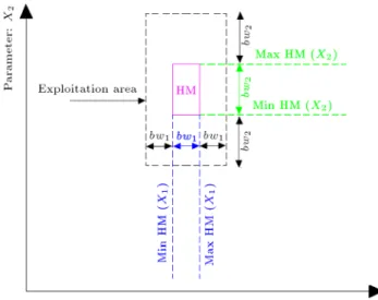
The bandwidth parameter (bw) serves for pitch-adjusting continuous design variables. Large values of bw should be used in the early optimization iterations to explore large regions of the design space thus approaching the global optimum. Conversely, small values of bw should be used in the nal optimization cycles where exploitation capability is required for performing ecient local search. In order to balance diversication in initial search steps and intensication in the nal search steps, bw must dynamically change during the search process. For that purpose, MAHS sets the bw parameter as:
bw(NI)=bwmin (bwmin bwmax)
1 max NINI 2
with probability Pbw; (15)
bw(NI) = [max(HMi) min(HMi)]
with probability (1 Pbw); (16)
where bwmax and bwmin are the maximum and
mini-mum bandwidth values, respectively; NI denotes the current improvisation (i.e. number of structural analy-ses); maxNI is the maximum number of improvisations; bw(NI) is the bandwidth distance used in the NIth improvisation; min(HMi) and max(HMi), respectively,
are the minimum and maximum values of the ith design variable stored in the HM matrix.
The value of bw determined from Eq. (15) de-creases quadratically with the number of improvisa-tions. Using quadratic variation will raise the reduction rate of the bw parameter relative to linear variation. This causes the bw parameter to approach faster to its minimum value (bwmin). By using this strategy,
exploitation capability required for performing ecient local search can be improved. In the early optimiza-tion cycles, HS explores large regions of design space
Figure 1. Illustration of the use of Eq. (16).
because the [max(HMi)-min(HMi)] dierence is large.
Thus, MAHS concentrates more on diversication. As the minimum and maximum values of the ith design variable stored in HM eventually approach the optimum, the [max(HMi)-min(HMi)] dierence tends
to become zero. Therefore, the optimization algorithm focuses more on intensication.
A new design vector is generated in the neigh-borhood of the harmony memory with Eq. (16); con-sequently, MAHS approaches quickly the region of design space containing the global optimum. Figure 1 illustrates this process for a 2D optimization problem. Besides values included in the HM matrix, neighboring values can be considered in the formation of the new solution.
If the pitch-adjusted value, anew
i , violates side
constraints, the value of the ith design variable is reset as follows:
anew
i amini + rand (aoldi amini )
if anew
i amini ; (17)
anew
i amaxi rand (amaxi aoldi )
if anew
i amaxi ; (18)
where aold
i is the value of the ith design variable before
pitch-adjusting; amin
i and amaxi , respectively, are the
corresponding side constraints.
4.1.2. Update of the new Pbw parameter
As the dierence of [max(HMi)-min(HMi)] approaches
zero in the nal search steps, the probability of choos-ing Eq. (16) should decrease. For that purpose, MAHS utilizes the new parameter Pbw to choose the equation
for updating bw. In particular, Pbw is dynamically
updated during the search process as:
Pbw(NI) = Pbw;min+Pbw;maxMax NIPbw;min NI: (19)
It appears that Pbw increases linearly in the
optimiza-tion process. A random number uniformly distributed in the interval (0,1) is generated. If this random number is smaller than Pbw, the value of bw is chosen
from Eq. (15), otherwise Eq. (16) is utilized. Therefore, MAHS is more likely to use Eq. (16) for updating bw in the initial iterations. Conversely, because Pbw
grad-ually increases towards the end optimization process, where Eq. (16) approaches zero, choosing Eq. (15) to update bw is more probable.
4.1.3. Update of the HMCR parameter
The HMCR and PAR parameters are used to improve the current solution. Unlike classic HS, the harmony memory considering rate parameter is dynamically updated in MAHS as:
HMCR(NI) =HMCRmin+(HMCRmax HMCRmin)
NI Max NI
0:1
: (20)
This causes the probability of choosing one value from historical values stored in the harmony memory to increase during the search process. The exponent 0.1 for Eq. (20), causes the value of HMCR to increase faster in the early optimization iterations. In other words, in the nal search steps, the new design variable is selected almost from the values stored in HM. This can enhance intensication in the nal search steps. The typical variation of HMCR versus the number of improvisations is shown in Figure 2.
4.1.4. Update of the PAR parameter
The pitch adjusting rate parameter, also, is dynami-cally updated in the search process. In particular, it decreases with the number of improvisations:
PAR(NI) =PARmax (PARmax PARmin)
NI Max NI
2
: (21)
Figure 2. Typical variation of HMCR with the number of improvisation.
By setting PAR to a large value, it is possible to increase the probability of pitch-adjusting the values selected from HM. This enhances the diversication ability of MAHS in the initial iterations. The PAR parameter reduces to its minimum value in the nal iterations, enough for performing local search that focuses more on intensication. By using this quadratic variation, the reduction rate of the PAR parameter increases in nal stage of search.
4.2. Discrete design variables
For optimization problems with discrete design vari-ables, Pbw, PAR, HMCR parameters are dened as in
Section 4.1 with only a dierence: the bandwidth bw is replaced by the neighboring index m, which is an integer number:
m(NI) =Ceil
mmin (mmin mmax)
1 Max NINI 2
with probability Pbw;
(22) m(NI) = [kmax(HMi) kmin(HMi)]
with probability (1 Pbw); (23)
where mmax and mmin are the maximum and
mini-mum neighboring index values, respectively; m(NI) is neighboring index in the NIth improvisation; \Ceil" is a function that is rounded up to the next highest integer; kmin(HMi) and kmax(HMi) are the bounds of the ith
discrete variable stored in the harmony memory. If the pitch adjusted value violates side con-straints, the value of optimization variable is reset with Eqs. (17) and (18) where amin
i and amaxi are replaced
by the corresponding discrete variable bounds. 5. Test problems and optimization results The new multi-adaptive harmony search algorithm developed in this research was tested in classical sizing optimization problems of trusses and frames. Opti-mum designs obtained by MAHS were compared in detail with other metaheuristic algorithms presented in literature. Furthermore, convergence behavior of MAHS was compared with the Global-Best Harmony Search (GHS) developed by Omran and Mahdavi [14], Self-Adaptive Harmony Search developed by Wang and Huang [15] and used by Degertekin [21], and Ecient Harmony Search, which is originally Improved Harmony Search, was presented by Mahdavi et al. [12] applied by Degertekin [21]. The best combination of internal parameters was determined by sensitivity analysis: PARmin = 0:2 0:3, PARmax = 0:7 0:8,
HMCRmin=0.9, HMCRmax=0.951.0, Pbw;min = 0:2
and Pbw;max = 0:8 1:0, HMS=10 20, mmin = 1
and mmax= 15.
In this paper, the parameters of the algorithms are not set initially. In all examples, sensitivity analyses are performed in order to nd an appro-priate set of parameters to obtain the best result. In sensitivity analysis we x all parameters except one and we study the variation of that particular parameter. We do this for other parameters to obtain the best combination of parameters; however it is not required to do this for all examples since the parameters set is almost the same in all the examples. Generally, in all examples, the parameters set is consid-ered as follows: PARmin=0.20.3, PARmax=0.70.8,
HMCRmin=0:9, HMCRmax=0.951.0, Pbw;min=0:2
and Pbw;max=0.81.0, HMS=1020, mmin = 1 and
mmax= 15.
5.1. Truss structures 5.1.1. Planar 10-bar truss
The rst test problem is the weight minimization of the planar 10-bar planar shown in Figure 3. The modulus of elasticity of the material is 10 Msi and material density is 0.1 lb/in3. The maximum stress for all
members was set as 25 ksi. The maximum allowable displacement for all free nodes in X and Y directions is set as 2.0 in. The cross-sectional area of each element was included as design variable; therefore, there are 10 sizing variables. The minimum cross-sectional area of all members is 0.1 in2.
Two dierent loading cases are considered. In Case 1, concentrated loads of 100 kips are applied at nodes 2 and 4 in the negative Y direction (i.e. P1= 100
kips and P2= 0). In Case 2, P1= 150 kips and P2= 50
kips hold.
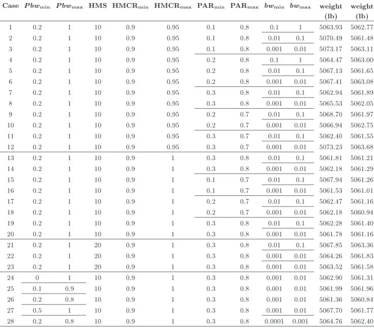
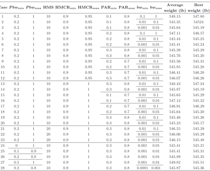
In order to evaluate the sensitivity of the MAHS algorithm to internal parameters, dierent combina-tions of internal parameters were considered and in-dependent optimization runs were carried for each combination starting from dierent initial populations. Table 1 shows the results of the sensitivity analysis performed for Case 1. Once the best combination of
Table 1. Sensitivity analysis to nd the best set of parameters of MAHS for the 10-bar truss (Case 1). Case P bwmin P bwmax HMS HMCRmin HMCRmax PARmin PARmax bwmin bwmax
Average weight
(lb)
Best weight
(lb)
1 0.2 1 10 0.9 0.95 0.1 0.8 0.1 1 5063.93 5062.77
2 0.2 1 10 0.9 0.95 0.1 0.8 0.01 0.1 5070.49 5061.48
3 0.2 1 10 0.9 0.95 0.1 0.8 0.001 0.01 5073.17 5063.11
4 0.2 1 10 0.9 0.95 0.2 0.8 0.1 1 5064.47 5063.00
5 0.2 1 10 0.9 0.95 0.2 0.8 0.01 0.1 5067.13 5061.65
6 0.2 1 10 0.9 0.95 0.2 0.8 0.001 0.01 5067.41 5063.08
7 0.2 1 10 0.9 0.95 0.3 0.8 0.01 0.1 5062.94 5061.89
8 0.2 1 10 0.9 0.95 0.3 0.8 0.001 0.01 5065.53 5062.05
9 0.2 1 10 0.9 0.95 0.2 0.7 0.01 0.1 5068.70 5061.97
10 0.2 1 10 0.9 0.95 0.2 0.7 0.001 0.01 5066.94 5062.75
11 0.2 1 10 0.9 0.95 0.3 0.7 0.01 0.1 5062.40 5061.55
12 0.2 1 10 0.9 0.95 0.3 0.7 0.001 0.01 5073.23 5063.68
13 0.2 1 10 0.9 1 0.3 0.8 0.01 0.1 5061.81 5061.21
14 0.2 1 10 0.9 1 0.3 0.8 0.001 0.01 5062.18 5061.29
15 0.2 1 10 0.9 1 0.1 0.7 0.01 0.1 5067.94 5061.26
16 0.2 1 10 0.9 1 0.1 0.7 0.001 0.01 5061.53 5061.01
17 0.2 1 10 0.9 1 0.2 0.7 0.01 0.1 5062.47 5061.16
18 0.2 1 10 0.9 1 0.2 0.7 0.001 0.01 5062.18 5060.94
19 0.2 1 10 0.9 1 0.3 0.8 0.01 0.1 5062.28 5061.40
20 0.2 1 10 0.9 1 0.3 0.8 0.001 0.01 5061.78 5061.16
21 0.2 1 20 0.9 1 0.3 0.8 0.01 0.1 5067.85 5063.36
22 0.2 1 20 0.9 1 0.3 0.8 0.001 0.01 5064.26 5061.83
23 0.2 1 20 0.9 1 0.3 0.8 0.001 0.01 5063.52 5061.58
24 0 1 10 0.9 1 0.3 0.8 0.001 0.01 5062.90 5061.31
25 0.1 0.9 10 0.9 1 0.3 0.8 0.001 0.01 5061.99 5061.96
26 0.2 0.8 10 0.9 1 0.3 0.8 0.001 0.01 5061.36 5060.84
27 0.5 1 10 0.9 1 0.3 0.8 0.001 0.01 5067.70 5061.77
28 0.2 0.8 10 0.9 1 0.3 0.8 0.0001 0.001 5064.76 5062.40
internal parameters was determined, 30 independent optimization runs were carried out starting from dif-ferent initial populations. The maximum number of improvisations was always set equal to 10,000.
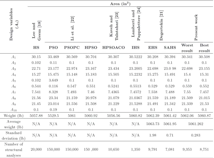
Tables 2 and 3 compare the optimization results obtained by MAHS with literature for Case 1 and Case 2, respectively. Statistical data such as the average weight and standard deviation of weight determined for 30 independent optimization runs are included in the table and the best and worst optimized weights obtained in the 30 optimization runs are also shown.
It can be seen that the present algorithm always converges to the best design without violating any optimization constraint. Furthermore, the worst design obtained in the 30 independent optimization runs was just slightly dierent from the optimized designs reported in literature. Standard deviation on optimized
weight was smaller than that found for the SAHS used by Degertekin [21]. This proves that in spite of its stochastic nature, MAHS was always able to correctly converge to the global optimum.
The best designs were obtained after only 8751 and 8325 structural analyses for Case 1 and Case 2, respectively. In Case 1, classic HS obtained the opti-mum design after 20,000 structural analyses while in Case 2, classic HS required 15,000 structural analyses. However, the SAHS utilized by Degertekin [21] required less structural analyses than MAHS; i.e., respectively, 7081 and 7267 vs. 8751 and 8325.
Converges behavior of MAHS is compared with other HS variants in Figure 4 for Case 1. The maximum number of structural analyses (i.e. number of improvisation) was always set equal to 10,000 for all HS variants.
Table 2. Optimization results obtained for Case 1 of the planar 10-bar truss problem. Area (in2)
Design
variables
(A
i
)
Lee
and
Geem
[18]
Li
et
al.
[22]
Ka
veh
and
T
alatahari
[23]
Lam
b
erti
and
P
appalettere
[24]
Degertekin
[21]
Presen
t
w
ork
HS PSO PSOPC HPSO HPSOACO IHS EHS SAHS Worst
result
Best result A1 30.15 33.469 30.569 30.704 30.307 30.5222 30.208 30.394 30.341 30.508
A2 0.102 0.11 0.1 0.1 0.1 0.1 0.1 0.1 0.1 0.1
A3 22.71 23.177 22.974 23.167 23.434 23.2005 22.698 23.0 98 22.698 23.155 A4 15.27 15.475 15.148 15.183 15.505 15.2232 15.275 15.491 15.4 15.31
A5 0.102 3.649 0.1 0.1 0.1 0.1 0.1 0.1 0.1 0.1
A6 0.544 0.116 0.547 0.551 0.5241 0.5513 0.529 0.529 0.559 0.552
A7 7.541 8.328 7.493 7.46 7.4365 7.4572 7.558 7.488 7.55 7.457
A8 21.56 23.34 21.159 20.978 21.079 21.0367 21.559 21.189 21.509 21.015 A9 21.45 23.014 21.556 21.508 21.229 21.5288 21.491 21.342 21.339 21.53
A10 0.1 0.19 0.1 0.1 0.1 0.1 0.1 0.1 0.1 0.1
Weight (lb) 5057.88 5529.5 5061 5060.92 5056.56 5060.82 5062.39 5061.42 5062.06 5060.87 Average
weight (lb) N/A N/A N/A N/A N/A N/A 5063.73 5061.95 5061.262
Standard
deviation (lb) N/A N/A N/A N/A N/A N/A 1.98 0.71 0.283
Number of structural
analyses
20,000 150,000 150,000 150 ,000 10,650 1,350 9,791 7,081 9,353 8,751
Note : 1 lb=4.45 N; 1 in2=6.452 cm2; N/A : Not Available.
Figure 4. Comparison of HS variants convergence curves obtained for Case 1 of the planar 10-bar truss problem.
It can be seen that the average optimization history of MAHS is very close to the best run. The convergence speed of MAHS was denitely higher than for the other HS variants. EHS outperformed classical HS while GHS was, by far, the worst HS-based optimizer.
5.1.2. Spatial 25- bar truss
The third test problem solved in this study was the weight minimization of the spatial 25-bar truss shown in Figure 5. The modulus of elasticity of the material is 10 Msi while material density is 0.1 lb/in3. Because
of structural symmetry about the X and Y axes, truss elements were grouped into 8 independent groups (i.e. there are 8 sizing design variables) as: (1) A1, (2) A2
A5; (3) A6 A9; (4) A10 A11, (5) A12 A13, (6)
A14 A17, (7) A18 A21, and (8) A22 A25.
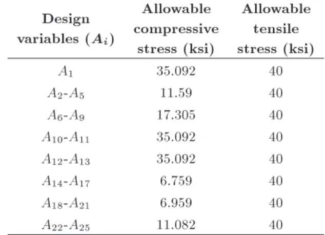
Stress limits in tension and compression for each element group are listed in Table 4. The maximum allowable displacement in every direction for all free nodes is 0.35 in. Cross-sectional areas of all elements must be less than 0.01 in2. The structure is subject
to two independent loading conditions described in Table 5.
Results of sensitivity analysis carried out for nding the best combination of internal parameters are presented in Table 6; ve independent runs were performed for each set of parameters. The table reports the best and average structural weights obtained by
Table 3. Optimization results obtained for Case 2 of the planar 10-bar truss problem. Area (in2)
Design
variables
(A
i
)
Sc
hmit
and
Farshi
[25]
Lee
and
Geem
[18]
Li
et
al.
[22]
Ka
veh
and
T
alatahari
[23]
Fesanghary
and
Mahda
vi
[16]
Degertekin
[21]
Presen
t
w
ork
HS PSO PSOPC HPSO HPSOACO SQPHS EHS SAHS Worst
result Best result A1 24.29 23.25 22.935 23.743 23.353 23.194 23.31 23.589 23.525 23.469 23.131
A2 0.1 0.102 0.113 0.101 0.1 0.1 0.1 0.1 0.1 0.1 0.1
A3 23.35 25.73 25.355 25.287 25.502 24.585 24.63 25.422 25.429 25.734 25.385 A4 13.66 14.51 14.373 14.413 14.25 14.221 14.59 14.488 14.488 14.031 14.338
A5 0.1 0.1 0.1 0.1 0.1 0.1 0.1 0.1 0.1 0.1 0.1
A6 1.969 1.977 1.99 1.969 1.972 1.969 1.967 1.975 1.992 1.971 1.97 A7 12.67 12.21 12.346 12.362 12.363 12.489 12.49 12.362 12.352 12.46 12.438 A8 12.54 12.61 12.923 12.694 12.984 12.925 12.94 12.682 12.698 13.24 13.138 A9 21.97 20.36 20.678 20.323 20.356 20.952 20.51 20.322 20.341 19.853 20.224
A10 0.1 0.1 0.1 0.103 0.101 0.101 0.1 0.1 0.1 0.1 0.1
Weight (lb) 4691.84 4668.81 4679.47 4677.7 4677.29 4675.78 4 668.72 4679.02 4678.84 4678.85 4677.71 Average
weight (lb) N/A N/A N/A N/A N/A N/A N/A 4681.61 4680.08 4678.8
Standard
deviation (lb) N/A N/A N/A N/A N/A N/A N/A 2.51 1.89 0.407
Number of structural
analyses
N/A 15,000 150,000 150,000 150,000 9,925 22,000 11,402 7,267 9,425 8,325
Figure 5. Schematic of the spatial twenty-ve-bar truss [18].
MAHS. In all cases, the maximum number of impro-visations (i.e. structural analysis) was set equal to 10,000.
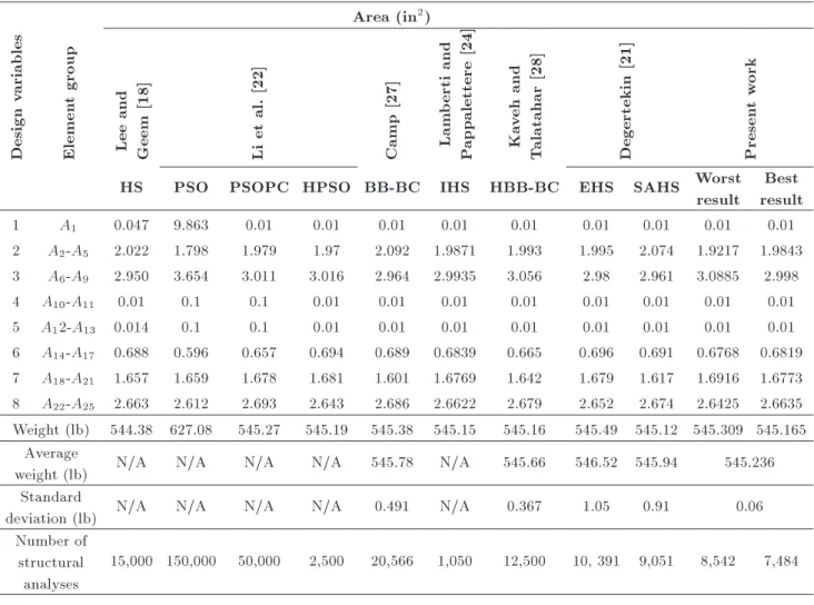
Table 7 compares the optimization results ob-tained by MAHS with literature. The SAHS algorithm
Table 4. Stress limits for the spatial 25-bar truss members.
Design variables (Ai)
Allowable compressive
stress (ksi)
Allowable tensile stress (ksi)
A1 35.092 40
A2-A5 11.59 40
A6-A9 17.305 40
A10-A11 35.092 40
A12-A13 35.092 40
A14-A17 6.759 40
A18-A21 6.959 40
A22-A25 11.082 40
used by Degertekin [21] obtains to the best design overall while the IHS algorithm developed by Lamberti and Pappalettere [24] is the fastest optimizer overall. The optimum design reported for classical HS [18] violated slightly the optimization constraints. Remark-ably, the worst result found in the 30 independent runs carried out for MAHS was practically the same as the best design found by the other optimization
algorithms. Similar to the previous examples, the stan-dard deviation on optimized weight found by MAHS was quite small. Classical HS obtained the optimum solution after 15,000 structural analyses while MAHS required only 7,484 structural analyses to complete the optimization process.
Convergence curves presented in Figure 6 conrm that MAHS has a better convergence behavior than other HS variants which rank as in the previous two test cases.
Table 5. Loading conditions for the spatial 25-bar truss (kips).
Node Condition 1 Condition 2
Fx Fy Fz Fx Fy Fz
1 0 20 -5 1 10 -5
2 0 -20 -5 0 10 -5
3 0 0 0 0.5 0 0
6 0 0 0 0.5 0 0
5.1.3. Spatial 72-bar truss
In the fourth test problem, the weight of the spatial 72-bar truss shown in Figure 7 is minimized. The modulus of elasticity of the material is 10 Msi and material density is 0.1 lb/in3. The cross-sectional areas of the
Figure 6. Comparison of HS variants convergence curves obtained for the spatial 25-bar truss problem.
Table 6. Results of sensitivity analysis carried for tuning the MAHS internal parameters for spatial 25-bar truss problem. Case P bwmin P bwmax HMS HMCRmin HMCRmax PARmin PARmax bwmin bwmax Average
weight (lb)
Best weight (lb)
1 0.2 1 10 0.9 0.95 0.1 0.8 0.1 1 548.15 547.80
2 0.2 1 10 0.9 0.95 0.1 0.8 0.01 0.1 545.35 54524
3 0.2 1 10 0.9 0.95 0.1 0.8 0.001 0.01 545.64 545.19
4 0.2 1 10 0.9 0.95 0.2 0.8 0.1 1 547.11 546.57
5 0.2 1 10 0.9 0.95 0.2 0.8 0.01 0.1 545.44 545.25
6 0.2 1 10 0.9 0.95 0.2 0.8 0.001 0.01 545.41 545.24
7 0.2 1 10 0.9 0.95 0.3 0.8 0.01 0.1 545.39 545.29
8 0.2 1 10 0.9 0.95 0.3 0.8 0.001 0.01 545.76 545.20
9 0.2 1 10 0.9 0.95 0.2 0.7 0.01 0.1 545.56 545.31
10 0.2 1 10 0.9 0.95 0.2 0.7 0.001 0.01 545.85 545.28
11 0.2 1 10 0.9 0.95 0.3 0.7 0.01 0.1 546.41 546.28
12 0.2 1 10 0.9 0.95 0.3 0.7 0.001 0.01 546.07 546.26
13 0.2 1 10 0.9 1 0.3 0.8 0.01 0.1 548.42 547.24
14 0.2 1 10 0.9 1 0.3 0.8 0.001 0.01 545.87 545.19
15 0.2 1 10 0.9 1 0.1 0.7 0.01 0.1 545.63 545.29
16 0.2 1 10 0.9 1 0.1 0.7 0.001 0.01 547.12 545.22
17 0.2 1 10 0.9 1 0.2 0.7 0.01 0.1 546.91 546.29
18 0.2 1 10 0.9 1 0.2 0.7 0.001 0.01 545.64 545.20
19 0.2 1 10 0.9 1 0.3 0.8 0.01 0.1 545.46 545.26
20 0.2 1 10 0.9 1 0.3 0.8 0.001 0.01 545.23 545.17
21 0.2 1 20 0.9 1 0.3 0.8 0.01 0.1 546.55 545.29
22 0.2 1 20 0.9 1 0.3 0.8 0.001 0.01 546.06 545.29
23 0.2 1 20 0.9 1 0.3 0.8 0.001 0.01 546.15 545.48
24 0 1 10 0.9 1 0.3 0.8 0.001 0.01 545.41 545.21
25 0.1 0.9 10 0.9 1 0.3 0.8 0.001 0.01 545.41 545.31
26 0.2 0.8 10 0.9 1 0.3 0.8 0.001 0.01 545.89 545.35
27 0.5 1 10 0.9 1 0.3 0.8 0.001 0.01 549.82 545.51
Table 7. Optimization results obtained for the planar 25-bar truss problem. Area (in2)
Design
variables
Elemen
t
group
Lee
and
Geem
[18]
Li
et
al.
[22]
Camp
[27]
Lam
b
erti
and
P
appalettere
[24]
Ka
veh
and
T
alatahar
[28]
Degertekin
[21]
Presen
t
w
ork
HS PSO PSOPC HPSO BB-BC IHS HBB-BC EHS SAHS Worst
result
Best result
1 A1 0.047 9.863 0.01 0.01 0.01 0.01 0.01 0.01 0.01 0.01 0.01
2 A2-A5 2.022 1.798 1.979 1.97 2.092 1.9871 1.993 1.995 2.074 1.9217 1.9843 3 A6-A9 2.950 3.654 3.011 3.016 2.964 2.9935 3.056 2.98 2.961 3.0885 2.998
4 A10-A11 0.01 0.1 0.1 0.01 0.01 0.01 0.01 0.01 0.01 0.01 0.01
5 A12-A13 0.014 0.1 0.1 0.01 0.01 0.01 0.01 0.01 0.01 0.01 0.01
6 A14-A17 0.688 0.596 0.657 0.694 0.689 0.6839 0.665 0.696 0.691 0.6768 0.6819 7 A18-A21 1.657 1.659 1.678 1.681 1.601 1.6769 1.642 1.679 1.617 1.6916 1.6773 8 A22-A25 2.663 2.612 2.693 2.643 2.686 2.6622 2.679 2.652 2.674 2.6425 2.6635 Weight (lb) 544.38 627.08 545.27 545.19 545.38 545.15 545.16 545.49 545.12 545.309 545.165
Average
weight (lb) N/A N/A N/A N/A 545.78 N/A 545.66 546.52 545.94 545.236 Standard
deviation (lb) N/A N/A N/A N/A 0.491 N/A 0.367 1.05 0.91 0.06
Number of structural
analyses
15,000 150,000 50,000 2,500 20,566 1,050 12,500 10, 391 9,051 8,542 7,484
Figure 7. Schematic of the spatial seventy-two-bar truss [18].
72 elements, taken as sizing variables, are divided into 16 groups, because of the structural symmetry about X and Y axes, as follows:
(1) A1 A4; (2) A5 A12,
(3) A13 A16; (4) A17 A18,
(5) A19 A22; (6) A23 A30,
(7) A31 A34; (8) A35 A36,
(9) A37 A40; (10) A41 A48,
(11) A49 A52; (12) A53 A54,
(13) A55 A58; (14) A59 A66,
(15) A67 A70; (16) A71 A72.
Therefore, the test problem has 16 design variables. This spatial truss is subject to two independent loading conditions shown in Table 8. The maximum stress for all members is 25,000 psi. The maximum displacement
of all free nodes in X and Y directions must be less than 0.25 in.
Two problem variants were considered. In Case 1, the minimum cross-sectional area of all members is 0.1 in2. In Case 2, the minimum cross-sectional area
of all members is 0.01 in2. Tables 9 and 10 report
Table 8. Loading conditions for the 72-bar spatial truss (kips).
Node Condition 1 Condition 2
Fx Fy Fz Fx Fy Fz
17 5 5 -5 0 0 -5
18 0 0 0 0 0 -5
19 0 0 0 0 0 -5
20 0 0 0 0 0 -5
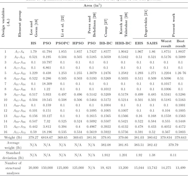
the optimization results and compare MAHS with literature. It can be seen from Table 9 that MAHS obtained the best feasible design. Remarkably, the worst result obtained in the 30 independent runs prac-tically coincides with the optimized weights reported in literature.
Table 10 shows that MAHS found the second best design, very close to that found by Lamberti with ecient simulated annealing [29]. Similar to previous examples, standard deviation on optimized weight was very small. In Case 1, classical HS required 20,000 structural analyses while MAHS converged to the optimum design within only 13,499 analyses. In Case 2, classical HS required 20,000 structural analyses while MAHS required only 12,298 analyses.
Convergence curves of HS variants are shown in
Table 9. Optimization results obtained for Case 1 of the spatial 72-bar truss problem. Area (in2)
Design
variables
(A
i
)
Elemen
t
group
Lee
and
Geem
[18]
Li
et
al.
[22]
P
erez
and
Behdinan
[26]
Camp
[27]
Ka
veh
and
T
alatahar
[28]
Degertekin
[21]
Presen
t
w
ork
HS PSO PSOPC HPSO PSO BB-BC HBB-BC EHS SAHS Worst
result
Best result 1 A1-A4 1.79 41.794 1.855 1.857 1.7427 1.8577 1.9042 1.967 1.86 1.8751 1.8837 2 A5-A12 0.521 0.195 0.504 0.505 0.5185 0.5059 0.5162 0.51 0.521 0.5176 0.5089
3 A13-A16 0.1 10.797 0.1 0.1 0.1 0.1 0.1 0.1 0.1 0.1 0.1
4 A17-A18 0.1 6.861 0.1 0.1 0.1 0.1 0.1 0.1 0.1 0.1 0.1
5 A19-A22 1.229 0.438 1.253 1.255 1.3079 1.2476 1.2582 1.293 1.271 1.2204 1.26 76 6 A23-A30 0.522 0.286 0.505 0.503 0.5193 0.5269 0.5035 0.511 0.509 0.5096 0.51
7 A31-A34 0.1 18.309 0.1 0.1 0.1 0.1 0.1 0.1 0.1 0.1017 0.1
8 A35-A36 0.1 1.22 0.1 0.1 0.1 0.1012 0.1 0.1 0.1 0.1006 0.1
9 A37-A40 0.517 5.933 0.497 0.496 0.5142 0.5209 0.5178 0.499 0.485 0.5341 0.5286 10 A41-A48 0.504 19.545 0.508 0.506 0.5464 0.5172 0.5214 0.501 0.501 0.5185 0.5163
11 A49-A52 0.1 0.159 0.1 0.1 0.1 0.1004 0.1 0.1 0.1 0.1 0.1001
12 A53-A54 0.101 0.151 0.1 0.1 0.1095 0.1005 0.1007 0.1 0.1 0.104 0.1005 13 A55-A58 0.156 10.127 0.1 0.1 0.1615 0.1565 0.1566 0.16 0.168 0.1558 0.1563 14 A59-A66 0.547 7.32 0.525 0.524 0.5092 0.5507 0.5421 0.522 0.584 0.555 0.5448 15 A67-A70 0.442 3.812 0.394 0.4 0.4967 0.3922 0.4132 0.478 0.433 0.4052 0.4172 16 A71-A72 0.59 18.196 0.535 0.534 0.5619 0.5922 0.5756 0.591 0.52 0.567 0.5803 Weight (lb) 379.27 6818.67 369.65 369.65 381.91 379.85 379.66 381.03 380.62 379.834 379.643
Average
weight (lb) N/A N/A N/A N/A N/A 382.08 381.85 383.51 382.42 379.79 Standard
deviation (lb) N/A N/A N/A N/A N/A 1.912 1.201 1.92 1.38 0.11
Number of structural
analyses
Table 10. Optimization results obtained for Case 2 of the spatial 72-bar truss problem. Area (in2)
Design variables
(Ai)
Element group
Lee and Geem [18]
Li et al. [22] Lamberti [29] Degertekin [21] Present work
HS PSO PSOPC HPSO CMLPSA EHS SAHS Worst
result
Best result 1 A1-A4 1.963 40.053 1.652 1.907 1.8866 1.889 1.889 1.8892 1.9202
2 A5-A12 0.481 0.237 0.547 0.524 0.5169 0.502 0.52 0.5167 0.5112
3 A13-A16 0.01 21.692 0.1 0.01 0.01 0.01 0.01 0.01 0.01
4 A17-A18 0.011 0.657 0.101 0.01 0.01 0.01 0.01 0.01 0.01
5 A19-A22 1.233 22.144 1.102 1.288 1.2903 1.284 1.289 1.3668 1.3144 6 A23-A30 0.506 0.266 0.589 0.523 0.517 0.526 0.524 0.5125 0.5082
7 A31-A34 0.011 1.654 0.011 0.01 0.01 0.01 0.01 0.01 0.01
8 A35-A36 0.012 10.284 0.01 0.01 0.01 0.01 0.01 0.01 0.01
9 A37-A40 0.538 0.559 0.581 0.544 0.5207 0.528 0.539 0.5244 0.5252 10 A41-A48 0.533 12.883 0.458 0.528 0.518 0.525 0.519 0.5204 0.5209
11 A49-A52 0.01 0.138 0.01 0.019 0.01 0.01 0.015 0.0119 0.0102
12 A53-A54 0.167 0.188 0.152 0.02 0.1141 0.063 0.105 0.0553 0.116 13 A55-A58 0.161 29.048 0.161 0.176 0.1665 0.173 0.167 0.1734 0.1663 14 A59-A66 0.542 0.632 0.555 0.535 0.5363 0.55 0.532 0.5101 0.5341 15 A67-A70 0.478 3.045 0.514 0.426 0.446 0.444 0.425 0.4664 0.4503 16 A71-A72 0.551 1.711 0.648 0.612 0.5761 0.592 0.579 0.6496 0.5695 Weight (lb) 364.33 5417.02 368.45 364.86 363.818 364.36 364.05 364.4837 363.8838
Average
weight (lb) N/A N/A N/A N/A N/A 366.79 366.57 364.017
Standard
deviation (lb) N/A N/A N/A N/A N/A 2.05 2.02 0.125
Number of structural
analyses
20,000 150,000 150,000 150, 000 900 13,755 12,852 12,935 12,298
Figure 8. Comparison of HS variants convergence curves obtained for Case 1 of the spatial 72-bar truss problem.
Figure 8 for Case 1. It can be seen that the average converge history of MAHS is very close to that obtained for the best run. MAHS was always faster than HS variants that ranked in the same fashion as for the previous test problems.
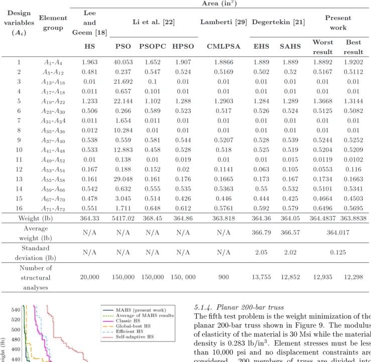
5.1.4. Planar 200-bar truss
The fth test problem is the weight minimization of the planar 200-bar truss shown in Figure 9. The modulus of elasticity of the material is 30 Msi while the material density is 0.283 lb/in3. Element stresses must be less
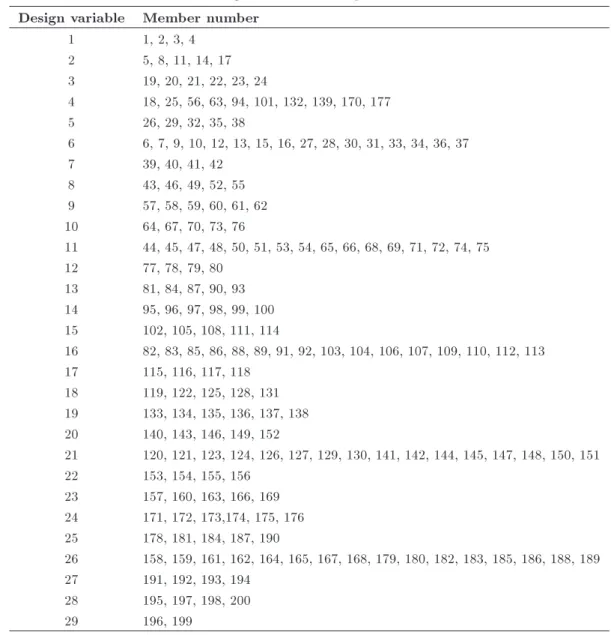
than 10,000 psi and no displacement constraints are considered. 200 members of truss are divided into 29 groups (see Table 11); therefore, this test problem consists of 29 sizing variables. The minimum cross-sectional area of all members was 0.1 in2. The structure
is subject to three independent loading conditions listed in Table 12.
Table 13 shows the optimum design found by MAHS and compares the present algorithm with litera-ture. MAHS converged to the best feasible design with a small standard deviation. The worst result obtained in the 10 independent runs performed for this test problem was consistent with other designs quoted in literature. Classical HS obtained the optimum design after 48,000 analyses while MAHS required only 21,235 analyses.
Table 11. Design variables for the planar 200-bar truss. Design variable Member number
1 1, 2, 3, 4 2 5, 8, 11, 14, 17 3 19, 20, 21, 22, 23, 24
4 18, 25, 56, 63, 94, 101, 132, 139, 170, 177 5 26, 29, 32, 35, 38
6 6, 7, 9, 10, 12, 13, 15, 16, 27, 28, 30, 31, 33, 34, 36, 37 7 39, 40, 41, 42
8 43, 46, 49, 52, 55 9 57, 58, 59, 60, 61, 62 10 64, 67, 70, 73, 76
11 44, 45, 47, 48, 50, 51, 53, 54, 65, 66, 68, 69, 71, 72, 74, 75 12 77, 78, 79, 80
13 81, 84, 87, 90, 93 14 95, 96, 97, 98, 99, 100 15 102, 105, 108, 111, 114
16 82, 83, 85, 86, 88, 89, 91, 92, 103, 104, 106, 107, 109, 110, 112, 113 17 115, 116, 117, 118
18 119, 122, 125, 128, 131 19 133, 134, 135, 136, 137, 138 20 140, 143, 146, 149, 152
21 120, 121, 123, 124, 126, 127, 129, 130, 141, 142, 144, 145, 147, 148, 150, 151 22 153, 154, 155, 156
23 157, 160, 163, 166, 169 24 171, 172, 173,174, 175, 176 25 178, 181, 184, 187, 190
26 158, 159, 161, 162, 164, 165, 167, 168, 179, 180, 182, 183, 185, 186, 188, 189 27 191, 192, 193, 194
28 195, 197, 198, 200
29 196, 199
Table 12. Loading conditions for the planar 200-bar truss problem (kips).
Loading conditions Nodes Amount of load
Condition (1) 1, 6, 15, 20, 29,34, 43, 48, 57, 62 and 71 1 kips in positive X direction
Condition (2)
1, 2, 3, 4, 5, 6, 8, 10, 12, 14, 15, 16, 17,
10 kips in negative Y direction 18,19, 20, 22, 24, 26, 28,29 30, 31, 32, 33,
34, 36, 38, 40, 42, 43, 44, 45, 46, 47, 48, 50, 52, 54, 56, 57, 58, 59, 60, 61, 62, 64, 66, 68, 70, 71, 72, 73, 74 and 75
Condition (3) Loading conditions (1) and (2) acting together.
The convergence curves, shown in Figure 10, prove that the average optimization history of MAHS is very close to that found for the best run. The present algorithm is denitely superior over other HS variants which ranked in the same order as in the previous examples.
Figure 11 shows the existing and allowable
ele-ment stress values for the loading conditions 1, 2 and 3, respectively.
5.2. Frame structures
5.2.1. Planar ten-story one-bay planar frame
The rst frame design problem solved in this study is the weight minimization of the one-bay ten-story
Table 13. Optimization results obtained for the planar 200-bar truss problem. Area (in2)
Design variables
(Ai)
Lee and Geem [18]
Lamberti [29] Kaveh and Talatahari [23] Degertekin [21] Present work
HS CMLPSA PSO PSOPC HPSOACO EHS SAHS Worst
result
Best result
1 0.1253 0.1468 0.8016 0.759 0.1033 0.15 0.154 0.1370 0.1411
2 1.0157 0.94 2.4028 0.9032 0.9184 0.946 0.941 1.0564 0.9775
3 0.1069 0.1 4.3407 1.1 0.1202 0.101 0.1 0.1001 0.1113
4 0.1096 0.1 5.6972 0.9952 0.1009 0.1 0.1 0.1001 0.1001
5 1.9369 1.94 3.9538 2.135 1.8664 1.945 1.942 1.9534 1.9451
6 0.2686 0.2962 0.595 0.4193 0.2826 0.296 0.301 0.2881 0.2969
7 0.1042 0.1 5.608 1.0041 0.1 0.1 0.1 0.1015 0.1006
8 2.9731 3.1042 9.1953 2.8052 2.9683 3.161 3.108 3.1136 3.1149
9 0.1309 0.1 4.5128 1.0344 0.1 0.102 0.1 0.1106 0.1003
10 4.1831 4.1042 4.6012 3.7842 3.9456 4.199 4.106 4.1136 4.118
11 0.3967 0.4034 0.5552 0.5269 0.3742 0.401 0.409 0.4162 0.4078
12 0.4416 0.1912 18.751 0.4302 0.4501 0.181 0.191 0.1472 0.1425
13 5.1873 5.4284 5.9937 5.2683 4.9603 5.431 5.428 5.4349 5.4325
14 0.1912 0.1 0.1 0.9685 1.0738 0.1 0.1 0.1327 0.1504
15 6.241 6.4284 8.1561 6.0473 5.9785 6.428 6.427 6.4348 6.4224
16 0.6994 0.5734 0.2712 0.7825 0.7863 0.571 0.581 0.5807 0.5782
17 0.1158 0.1327 11.152 0.592 0.7374 0.156 0.151 0.2574 0.1691
18 7.7643 7.9717 7.1263 8.1858 7.3809 7.961 7.973 7.9871 7.9777
19 0.1 0.1 4.465 1.0362 0.6674 0.1 0.1 0.2851 0.1001
20 8.8279 8.9717 9.1643 9.2062 8.3 8.959 8.974 8.9867 8.9792
21 0.6986 0.7049 2.7617 1.4774 1.1967 0.722 0.719 0.9214 0.7423
22 1.5563 0.4196 0.5541 1.8336 1.0 0.491 0.422 0.6071 0.4615
23 10.9806 10.8636 16.164 10.611 10.8262 10.909 10.892 11.3988 10.9658
24 0.1317 0.1 0.4974 0.9851 0.1 0.101 0.1 0.1828 0.1002
25 12.1492 11.8606 16.225 12.509 11.6976 11.985 11.887 12.4178 11.9658
26 1.6373 1.0339 1.0042 1.9755 1.388 1.084 1.04 1.3514 1.0849
27 5.0032 6.6818 3.6098 4.5149 4.9523 6.464 6.646 5.2179 6.2849
28 9.3545 10.8113 8.3684 9.8 8.8 10.802 10.804 9.9046 10.7115
29 15.0919 13.8404 15.562 14.531 14.6645 13.936 13.87 14.7564 13.9967 Weight (lb) 25447.1 25445.63 44081.4 28537.8 25156.5 25542.5 25491.9 25650 25482.21
Average
weight (lb) N/A N/A N/A N/A N/A 25659.71 25610.2 25545.11
Standard
deviation (lb) N/A N/A N/A N/A N/A 164.17 148.85 49.69
Number of structural
analyses
48,000 9,650 150,000 150,000 9,875 22,851 19,670 22,425 21,235
frame shown in Figure 12. The modulus of elasticity is 29 Msi while yield stress is 36 ksi. The frame includes 30 members connected by 22 joints. Because of structural symmetry, elements are grouped in 5 groups of columns and 4 groups of beams (see Figure 12). This test problem included discrete optimization variables.
Cross-sectional areas of beam elements can be selected from 267 W -sections, while cross-sectional areas of columns can be selected from W 14 and W 12 sections.
The frame was previously optimized by Pezeshk et al. [30] using GA and by Camp et al. [31] using ACO. The eective length factors of members were
Figure 9. Schematic of planar 200-bar truss [21].
Figure 10. Comparison of HS variants convergence curves obtained for the planar 200-bar truss problem.
calculated as Kx 1 for sway-permitted frame using
the approximate equation developed by Dumonteil [32], whereas the out-of-plane length factor is Ky = 1. For
each beam member, the out-of-plane eective length factor was set as Ky= 0:2.
Table 14 compares the optimum design found by MAHS with literature. It can be seen that the present algorithm converged to a feasible design weighing 63,322 lb which is 2.78% lighter than the
Figure 11. Comparison of the allowable and existing element stresses for the planar 200-bar truss problem using the MAHS.
Table 14. Optimization results obtained for the ten-story one-bay frame problem. Section
Design variables Pezeshk et al. [30]
Camp
et al. [31] Degertekin [33]
Present work
GA ACO HS Worst
result
Best result
Columns
1 W 14 233 W 14 233 W 14 211 W 14 233 W 14 233 2 W 14 176 W 14 176 W 14 176 W 14 176 W 14 176 3 W 14 159 W 14 145 W 14 145 W 14 159 W 14 159
4 W 14 99 W 14 99 W 14 90 W 14 99 W 14 99
5 W 12 79 W 12 65 W 14 61 W 12 65 W 12 65
Beams
6 W 33 118 W 30 108 W 33 118 W 36 135 W 33 118
7 W 30 90 W 30 90 W 30 99 W 30 99 W 30 90
8 W 27 84 W 27 84 W 24 76 W 27 84 W 27 84
9 W 24 55 W 21 44 W 18 46 W 21 55 W 21 55
Weight (lb) 65,136 62,610 61,864 64,390 63,322
Average weight (lb) N/A N/A 62923 64129
Standard
deviation (lb) N/A N/A 1.74 219
Number of
structural analyses 3,000 8,300 3,690 2,555 1,095
optimum design found by GA [30]. Furthermore, the standard deviation of 20 dierent runs was very small: only 219 lb. GA [30], ACO [31] and classical HS [33] completed the optimization process within, respectively, 3000, 8300 and 3690 structural analyses while MAHS required only 1095 structural analyses.
The number of structural analyses required in the worst optimization run is higher than that required in the best optimization run. A possible reason for such a behavior is in the discrete nature of the frame problems. Convergence curves of HS variants are compared in Figure 13 for a maximum number of structural analyses set as 3,500 for all algorithms. Sensitivity analysis was performed for all HS variants and 20 independent optimization runs were then conducted
Figure 13. Comparison of HS variants convergence curves obtained for the ten-story one-bay frame problem.
starting from dierent initial designs. It can be seen that the average convergence curve of MAHS is very close to that obtained for the best optimization run. The present algorithm was the fastest HS variant followed by SAHS.
In Figure 14, inter-story drift for each story is
de-Figure 14. Comparison of the allowable and existing inter-story drift for the ten-story one-bay frame problem using the MAHS.
Figure 15. Comparison of the allowable and existing element stresses for the ten-story one-bay frame problem using the MAHS.
picted and compared to the allowable drift value. The maximum inter-story drift evaluated for the optimized design was 99.5% of the allowable value at the fth story. The global sway at the top story was 3.98 in, less than the maximum permitted sway (4.92 in). Element stresses also were smaller than the corresponding limit shown in Figure 15.
5.2.2. Planar twenty four-story three-bay frame The second test case with discrete variables was the weight minimization of the 3-bay 24-story frame shown in Figure 16. The frame included 100 joints connected by 168 elements. The modulus of elasticity of the material is E = 29; 732 ksi (205 GPa) and the yield stress is fy= 33; 400 psi (230.3 MPa). The columns in
a story are grouped in two groups of exterior columns and interior columns. Furthermore, columns belonging to three adjacent stories are grouped together. The beams of each story are divided into two groups as beam of inner bay and beams of outer bays. Beams are grouped together for all stories except the roof. Therefore, the 168 frame elements can be divided in 20 groups and the optimization problem includes 20 sizing variables. Cross-sectional areas of the 4 groups of beams can be selected from all 267 W -sections, while cross-sectional areas of the 16 groups of columns can be selected only from W 14 sections (37 W -shapes). The frame is subjected to the loads listed in Table 15. The structure is designed according the AISC-LRFD specications [19] with an inter-story drift displacement constraint. The eective length factors of the members are calculated as Kx 0 for a
sway-permitted frame using the approximate equation proposed by Dumonteil [32]. The out-of-plane eective length factor is specied as Ky = 1:0. All columns
and beams are considered as non-braced along their lengths.
Table 16 compares the MAHS optimum design with literature. The proposed algorithm converged to the best design without violating optimization con-straints. The worst design obtained in the 10 indepen-dent optimization runs carried out from dierent initial populations is better than the other designs reported in
Figure 16. Schematic of the twenty four-story three-bay frame [33].
literature. The standard deviation on optimized weight was only 1320 lb, smaller than for CSS. The MAHS algorithm required only 7115 structural analyses, hence less than ACO [31], HS [33] and ICA [35].
Optimization histories of HS variants are com-pared in Figure 17 for a maximum number of structural analyses equal to 14,000. Sensitivity analysis was carried out for each HS algorithm to nd the best combination of internal parameters, and 10 indepen-dent optimization runs were carried out starting from dierent initial populations. The convergence curves relative to the best optimization run are shown for each HS variant. Remarkably, the average convergence
curve of MAHS was better than the best convergence curves obtained for the other HS variants.
The optimized design fully satised the optimiza-tion constraints. Figure 18 shows the inter-story drift for each story and compares to the allowable drift value.
Table 15. Loading conditions for the twenty four-story three-bay frame problem.
Type Amount
W Lateral Left joints 5761.85 (lb) w1
Gravity
Roof beams 300 (lb/ft) w2 Left outer beams 436 (lb/ft)
w3 Inner beams 474 (lb/ft)
w4 Right outer beams 408 (lb/ft)
Figure 17. Comparison of HS variants convergence curves obtained for the twenty four-story three-bay frame problem.
Table 16. Optimization results obtained for the twenty four-story three-bay frame problem. Section
Design variables
Camp
et al. [31] Degertekin [33] Kaveh and Talatahari Present work
ACO HS IACO [34] ICA [35] CSS [36] Worst
result
Best result
Beams
1 W 30 90 W 30 90 W 30 99 W 30 90 W 30 90 W 30 90 W 30 90 2 W 8 18 W 10 22 W 16 26 W 21 50 W 21 50 W 12 68 W 10 49 3 W 24 55 W 18 40 W 18 35 W 24 55 W 21 48 W 24 44 W 21 48 4 W 8 21 W 12 16 W 14 22 W 8 28 W 12 19 W 14 19 W 12 40
Columns
5 W 14 145 W 14 176 W 14 145 W 14 109 W 14 176 W 14 233 W 14 176 6 W 14 132 W 14 176 W 14 132 W 14 159 W 14 145 W 14 145 W 14 145 7 W 14 132 W 14 132 W 14 120 W 14 120 W 14 109 W 14 109 W 14 109 8 W 14 132 W 14 109 W 14 109 W 14 90 W 14 90 W 14 61 W 14 74 9 W 14 68 W 14 82 W 14 48 W 14 74 W 14 74 W 14 53 W 14 61 10 W 14 53 W 14 74 W 14 48 W 14 68 W 14 61 W 14 53 W 14 61 11 W 14 43 W 14 34 W 14 34 W 14 30 W 14 34 W 14 30 W 14 30 12 W 14 43 W 14 22 W 14 30 W 14 38 W 14 34 W 14 22 W 14 22 13 W 14 145 W 14 145 W 14 159 W 14 159 W 14 145 W 14 90 W 14 99 14 W 14 145 W 14 132 W 14 120 W 14 132 W 14 132 W 14 99 W 14 109 15 W 14 120 W 14 109 W 14 109 W 14 99 W 14 109 W 14 109 W 14 99 16 W 14 90 W 14 82 W 14 99 W 14 82 W 14 82 W 14 120 W 14 90 17 W 14 90 W 14 61 W 14 82 W 14 68 W 14 68 W 14 90 W 14 74 18 W 14 61 W 14 48 W 14 53 W 14 48 W 14 43 W 14 53 W 14 53 19 W 14 30 W 14 30 W 14 38 W 14 34 W 14 34 W 14 43 W 14 34 20 W 14 26 W 14 22 W 14 26 W 14 22 W 14 22 W 14 26 W 14 26 Weight (lb) 220,465 214,860 217,475 212,735 212,459 211,172.9 206,224.9
Average weight (lb) 229,552 222,620 N/A N/A 215,313 208,776
Standard
deviation (lb) 4561 5800 N/A N/A 2448 1320
Number of structural
analyses
Figure 18. Comparison of the allowable and existing inter-story drift for the twenty four-story three-bay frame problem using the MAHS.
Figure 19. Comparison of the allowable and existing element stresses for the twenty four-story three-bay frame problem using the MAHS.
The global sway at the top story was 10.31 in, less than the maximum permitted sway (11.52 in).
In Figure 19, the existing and allowable element stresses for each member are shown. Inter-story drift governed the design process while stress constraints were less critical.
6. Concluding remarks
This study presented an improved Harmony Search algorithm termed as Multi-Adaptive Harmony Search (MAHS). The internal parameters of MAHS are
adap-tively modied to improve robustness and convergence behavior with respect to classical HS and other HS variants recently published in literature.
The new proposed algorithm was successfully utilized in sizing optimization problems of truss and frame structures with continuous and discrete design variables. The new mechanism of pitch-adjusting introduced in MAHS leads to obtain better results and faster convergence because the diversication and intensication stages of the optimization search process are very well balanced. Consequently, the computa-tional cost of MAHS is considerably smaller than other HS variants. Furthermore, the standard deviation of optimized weight over independent runs carried out starting from dierent initial populations is very small. Acknowledgments
The rst author is grateful to the Iran National Science Foundation for the support.
References
1. Osman, I.H. and Laporte, G. \Metaheuristics: A bibliography", Annals of Operations Research, 63(5), pp. 513-623 (1996).
2. Holland, J.H., Adaptation in Natural and Articial Systems, MIT Press Cambridge, MA, USA (1992).
3. Goldberg, D.E., Genetic Algorithms in Search Op-timization and Machine Learning, Addison-Wesley, Boston, MA, USA (1989).
4. Glover, F. \Heuristic for integer programming using surrogate constraints", Decision Sciences, 8(1), pp. 156-166 (1977).
5. Dorigo, M., Maniezzo, V. and Colorni A. \The ant system: Optimization by a colony of cooperating agents", IEEE Transactions on Systems, Man, and Cybernetics, Part B, 26(1), pp. 29-41 (1996).
6. Eberhart, R.C. and Kennedy, J. \A new optimizer using particle swarm theory", In: Proceedings of the Sixth International Symposium on Micro Machine and Human Science, Nagoya, Japan, IEEE Press, Piscat-away, NJ, pp. 39-43 (1995).
7. Kirkpatrick, S., Gelatt, C.D. and Vecchi, M.P. \Opti-mization by simulated annealing", Science, 220(4598), pp. 671-680 (1983).
8. Erol, O.K. and Eksin, I. \New optimization method: Big bang-big crunch", Advances in Engineering Soft-ware, 37(2), pp. 106-111 (2006).
9. Kaveh, A. and Talatahari, S. \A novel heuristic optimization method: Charged system search", Acta Mechanica, 213(3-4), pp. 267-289 (2010).
10. Geem, Z.W., Kim, J.H. and Loganathan, G.V. \A new heuristic optimization algorithm: Harmony search", Simulation, 76(2), pp. 60-68 (2001).
11. Geem, Z.W. \State-of-the-art in the structure of harmony search algorithm", in: Recent Advances in Harmony Search Algorithm, Studies in Computational Intelligence, 270, pp. 1-10 (2010).
12. Mahdavi, M., Fesanghary, M. and Damangir, E. \An improved harmony search algorithm for solving opti-mization problems", Applied Mathematics and Com-putation, 188(2), pp. 1567-1579 (2007).
13. Geem, Z.W. \Novel derivative of harmony search algorithm for discrete design variables", Applied Math-ematics and Computation, 199(1), pp. 223-230 (2008).
14. Omran, M.G.H. and Mahdavi, M. \Global-best har-mony search", Applied Mathematics and Computation, 198(2), pp. 643-656 (2008).
15. Wang, C.M. and Huang, Y.F. \Self-adaptive harmony search algorithm for optimization", Expert Systems with Applications, 37(4), pp. 2826-2837 (2010).
16. Fesanghary, M., Mahdavi, M., Minary-Jolandan, M. and Alizadeh, Y. \Hybridizing harmony search algo-rithm with sequential quadratic programming for engi-neering optimization problems", Computer Methods in Applied Mechanics and Engineering, 197(33-40), pp. 3080-3091 (2008).
17. Saka, M.P. and Hasancebi, O. \Adaptive harmony search algorithm for design code optimization of steel structures, harmony search algorithms for structural design optimization", In: Studies in Computational Intelligence, Geem, Z.W, Ed., 239, Berlin, Heidelberg: Springer-Verlag, pp. 79-120 (2009).
18. Lee, K.S. and Geem, Z.W. \A new structural opti-mization method based on the harmony search algo-rithm", Computers and Structures, 82(9-10), pp. 781-798 (2004).
19. American Institute of Steel Construction (AISC), Manual of Steel Construction-Load Resistance Factor Design, 2nd Ed, Chicago, AISC (1992).
20. Kaveh, A., Farahmand Azar, B. and Talatahari, S. \Ant colony optimization for design of space trusses", International Journal of Space Structures, 23(3), pp. 167-81 (2008).
21. Degertekin, S.O. \Improved harmony search algo-rithms for sizing optimization of truss structures", Computers and Structures, 92-93, pp. 229-241 (2012).
22. Li, L.J., Huang, Z.B., Liu, F. and Wu, Q.H. \A heuristic particle swarm optimizer for optimization of pin connected structures", Computers and Structures, 85(7-8), pp. 340-349 (2007).
23. Kaveh, A. and Talatahari, S. \Particle swarm opti-mizer, ant colony strategy and harmony search scheme hybridized for optimization of truss structures", Com-puters and Structures, 87(5-6), pp. 267-283 (2009).
24. Lamberti, L. and Pappalettere, C. \An improved harmony-search algorithm for truss structure optimiza-tion", In: Proceedings of the Twelfth International Conference Civil, Structural and Environmental En-gineering Computing, Topping, B.H.V., Neves, L.F.C. and Barros, R.C., Eds., Stirlingshire, Scotland: Civil-Comp Press (2009).
25. Schmit Jr, L.A. and Farshi, B. \Some approximation concepts for structural synthesis", American Institute of Aeronautics and Astronautics Journal, 12(5), pp. 692-699 (1974).
26. Perez, R.E. and Behdinan, K. \Particle swarm ap-proach for structural design optimization", Computers and Structures, 85(19-20), pp.1579-1588 (2007).
27. Camp, C.V. \Design of space trusses using big bang-big crunch optimization", Journal of Structural Engi-neering (ASCE), 133(7), pp. 999-1008 (2007).
28. Kaveh, A. and Talatahari, S. \Size optimization of space trusses using big-bang big-crunch algorithm", Computers and Structures, 87(17-18), pp. 1129-1140 (2009).
29. Lamberti, L. \An ecient simulated annealing algo-rithm for design optimization of truss structures", Computers and Structures, 86(19-20), pp. 1936-1953 (2008).
30. Pezeshk, S., Camp C.V. and Chen, D. \Design of non-linear framed structures using genetic optimization", Journal of Structural Engineering (ASCE), 126, pp. 382-388 (2000).
31. Camp, C.V., Bichon, B.J. and Stovall, S.P. \Design of steel frames using ant colony optimization", Journal of Structural Engineering (ASCE), 131, pp. 369-379 (2005).
32. Dumonteil, P. \Simple equations for eective length factors", Journal of Structural Engineering (ASCE), 3, pp. 111-115 (1992).
33. Degertekin, S.O. \Optimum design of steel frames using harmony search algorithm", Structural and Mul-tidisciplinary Optimization, 36(4), pp. 393-401 (2008).
34. Kaveh, A. and Talatahari, S. \An improved ant colony optimization for design of planar steel frames", Engi-neering Structures, 32(3), pp. 864-876 (2010).
35. Kaveh, A. and Talatahari, S. \Optimum design of skeletal structures using imperialist competitive al-gorithm", Computers and Structures, 88(21-22), pp. 1220-1229 (2010).
36. Kaveh, A. and Talatahari, S. \Charged system search for optimal design of frame structures", Applied Soft Computing, 12(1), pp. 382-393 (2012).
Biographies
Ali Kaveh was born in 1948 in Tabriz, Iran. After graduation from the Department of Civil Engineering at the University of Tabriz in 1969, he continued his studies on Structures at Imperial College of Science and Technology at London University, and received his MS, DIC and PhD degrees in 1970 and 1974, respectively. He then joined the Iran University of Science and Technology in Tehran where he is presently Professor of Structural Engineering. Professor Kaveh is the author of 420 papers published in international journals and 135 papers presented at international
conferences. He has authored 23 books in Farsi and 7 books in English published by Wiley, the American Me-chanical Society, Research Studies Press and Springer-Verlag.
Mohammad Naeimi was born in 1986 in Tehran, Iran. He obtained his BS degree in Civil Engineering from Khajeh Nasir Toosi University of Technology
(KNTU) in 2010, and received his MS degree in Earth-quake Engineering from Road, Housing and Urban Development Research Centre in 2013. At present, he studies on optimal design of structures with frequency constraints. His main research interests include: Struc-tural optimization, topology optimization, strucStruc-tural dynamics, seismic fragility of structural systems and soil-structure interaction.
![Table 13. Optimization results obtained for the planar 200-bar truss problem. Area (in 2 ) Design variables (A i ) Leeand Geem [18]](https://thumb-us.123doks.com/thumbv2/123dok_us/8387404.2228534/15.892.102.820.162.1027/table-optimization-results-obtained-problem-design-variables-leeand.webp)
