Sharif University of Technology
Scientia IranicaTransactions E: Industrial Engineering www.scientiairanica.com
A new method based on the multi-segment decision
matrix for solving decision-making problems
M. Salimi
a, B. Vahdani
a;, S.M. Mousavi
band R. Tavakkoli-Moghaddam
ca. Faculty of Industrial and Mechanical Engineering, Qazvin Branch, Islamic Azad University, Qazvin, P.O. Box 3419759811, Iran. b. Young Researches Club, South Tehran Branch, Islamic Azad University, Tehran, P.O. Box 11365/4435, Iran.
c. Department of Industrial Engineering, College of Engineering, University of Tehran, Tehran, P.O. Box 11155-4563, Iran. Received 20 October 2012; received in revised form 18 March 2013; accepted 15 July 2013
KEYWORDS Multi-Criteria Decision Making (MCDM); Multi-segment Multiple Attributes Decision-Making (MADM); Simple Additive Weight (SAW) method; Multi-segment decision-making matrix.
Abstract.Decision-making analysis methods are employed to nd the best option among feasible alternatives where an amount of alternatives versus criteria is introduced as only one value level with stationary numerical value. In real-world decision situations, the condition of multi-segment problems may exist in practice. In this paper, a new method is proposed to rank the alternatives in Multiple Criteria Decision-Making (MCDM) problems, where the amount of alternatives to the criteria can be represented by several segments. Hence, a multi-segment decision matrix can be obtained. Moreover, the proposed method, based on Simple Additive Weight (SAW), can be employed to solve the decision problems, where the amount of alternatives versus the assessment criteria at each level is introduced as a function of some parameters. These functions can be regarded as linear, exponential, and trigonometric. Finally, three real case studies are given to demonstrate the solution procedure of the proposed method, and then a sensitivity analysis for each case is reported.
c
2013 Sharif University of Technology. All rights reserved.
1. Introduction
Decision-making methods are utilized to nd the best option among all feasible alternatives. There are many methods to solve MCDM problems. Priority-based, outranking, distance-based and mixed methods are nominated as the principal classes of the MCDM [1,2]. The SAW method is one of the most diused ap-proaches in MCDM problems to have been widely used in real-life situations [3,4]. This method was rst utilized by Churchman and Acko (1945) to nd the best option for portfolio problems. The SAW is applied to evaluate the methods and to identify
*. Corresponding author. Tel: +98 281 3665275; Fax: +98 281 3670051
E-mail addresses: [email protected] (M. Salimi); [email protected] (B. Vahdani);
[email protected] (S.M. Mousavi); [email protected] (R. Tavakkoli-Moghaddam)
the best one according to its simplicity and general acceptability [5]. The basic principle of this method is to calculate a weighted sum of performance ratings of alternatives versus several criteria [6,7]. The SAW is known to be the most used, intuitive, and easy [7,8]. The method includes two basic steps: rst, calculating the values of all criteria to make them comparable, and second, summing up the values of all criteria for each alternative [9,10]. One important advantage of the SAW method is that the transformation of the raw data is linear. It means that the relative order of magnitude of the standardized scores remains equal [7].
In the past two decades, decision-making methods have provided a logical approach to analyze decision alternatives, where the amount of alternatives versus criteria is presented as a constant numerical value in the decision matrix. Thus, they are proposed with only one value level. To cope with many real-decision situations, the orientation of preference alternatives with respect
to criteria may not be the same as the preference with decision-making problems. The preference is presented as one value level in every condition. In other words, the decision-making variables are adjusted according to some parameters, such as demand rate for the buyer, business volume, price, quality, and delivery lead time. In recent years, many multi-segment, Multi-Objective Decision-Making (MODM) problems have been stud-ied, where the decision variables coecients are applied with dierent contribution levels or aspiration levels are proposed as a multi-segment problem, for example the basic price of products or services often adjusted by companies to accommodate dierences in customer, products, locations, etc. [11,12].
Multi-segment Multiple Attributes Decision-Making (MADM) problems, as the above-mentioned MODM problem, are available in the literature, but no methods of solving multi-segment MADM problems exist. There are many situations in which the multi-segment decision levels of the ith alternative versus the jth criterion (attribute) can be applied. For example, business volume discounts (e.g., the discounted price of allocated items to the alternatives) are applied to motivate the investors, corresponding to business volume. Producers give discounts (e.g., a reduction in the basic price of goods or services) in order to sell their products quickly and mostly give discounts to attract customers. In incremental discounts and all-unit discounts, xed and variable purchase costs are presented as the amount of alternatives. The parameters in current methods include stationary over time, order quantity and amount of production. It is pointed out that the xed order cost for the incremental discount can be dierent for each price break region; in other words, the incremental discount has several dierent costs [13]. The amounts of multi-segment decision matrix are in the kij amount levels for each alternative, Ai, with respect to criterion, Cj. Moreover, in some cases, some Decision Makers (DMs) believe that there may exist a situation where the amount of alternatives at each level can be presented as a function of some variables (above-denoted parameters); however, the DMs are not able to decide alternatives using current methods.
This paper proposes a new SAW method for the preference of alternatives with a multi-level deci-sion matrix based on the above-mentioned concepts. This method is frequently applied in real-life decision-making problems. In addition, the proposed model aims to determine the preference of the options, where the amount of decision matrix is presented as a function that is changed at k levels. It means that the value of each alternative can be changed versus each criterion at k levels. The value of k for each element of the decision matrix can be dierent. In other words, Kij levels for the ith alternative related to the jth criterion can be
considered. Therefore, two main contributions in this paper are as follows:
The proposed method leads to determine the pref-erence of alternatives in multi-segment problems which can be easily solved, step by step.
This method can be applied where the amount of alternatives at each level can be presented as a function of some variables. Thus, the functional amounts can be compared with each other.
Some functions are utilized in the decision-making matrix, such as linear, exponential, and trigonometric. A discount function is used in economic models. The overlapping of two curves may exist; the alternatives are ranked by considering the relation between the price break and the amount of these proposed func-tions. The preference of alternatives is presented in each interval as mentioned above. Therefore, the DM can prefer the options in all intervals, and then the decision-making can be done. The distance of deci-sion making can be broken down to several intervals, according to some conditions; the functional amount of alternative Ai versus criterion Cj at the kth level, and x is the variable that depends on an amount of some parameters, such as time, order quantity, and amount of production. For alternative Ai, with respect to criterion Cj, at the kth level, x belongs to [Lijkij; Uijkij].
In the previous methods, the DMs made decisions about the alternatives only once. However, regarding the changes, the previous methods cannot consider these changes throughout the decision-making process. Also, the value of each alternative with respect to each criterion can be a function of dierent variables instead of a number. In addition, since values of every column (attribute) in the decision-making matrix are normalized, all values are between 0 and 1. Thus, the criteria of the decision matrix can be taken as any various types. Further, since the area under the curve of the function is utilized for the nal value of the decision matrix, this method can be employed when the DMs are not aware of the exact values of the alternatives, although they know that the values are in the [a; b] interval.
There are some advantages of the multi-segment SAW method, which are provided as below:
1. The SAW is very easy and the proposed method is presented step by step; therefore, the computation process is simple and straightforward.
2. The DMs can nd the best alternative in each interval form.
3. In some cases, the overlapping of two curves with each other may exist; hence, the preference of alternatives may be changed in each interval. Con-sidering this concept, the new method proposes a
logical mathematical tool to help the DMs in order to make the best decision.
4. During this multi-segment approach, there is one parameter available to deal with decision problems. Many parameters can be introduced in real-life application, such as time, order quantity, and the amount of production.
5. This method can help the DM when the order quantity of alternatives is not exactly determinable, and the bounds of the order quantity are assigned as an interval form.
6. In this method, values of alternatives versus criteria are transformed into a dimensionless value. Thus, the nal value of alternatives can be calculated, where the attributes are presented by dierent dimensions.
The remainder of this paper is organized as follows. The SAW method is presented in the next section. In Section 3, the procedure of ranking by the proposed SAW method with a multi-segment decision matrix is described. In Section 4, the three important functions used in the case study are described. In Section 5, three case studies, including the preference of three mechanical engines, to nd the best option among three companies and suitable institutes among three alterna-tives, are provided. Then, the sensitivity analysis is described for each case. The last section is devoted to conclusions.
2. SAW method
Suppose a decision-making problem has n alterna-tives, A1; A2; ; An and m criteria, C1; C2; ; Cm. Each alternative is evaluated with respect to the m criteria. All the alternatives' performances related to each criterion from a decision matrix are denoted by a = [aij]nm. Let W = (w1; w2; ; wm) be the relative vector presenting the criteria weights, satisfyingPmj=1wj = 1, then, the process of the SAW method consists of the following steps [14]:
Step 1. Construct the decision-making matrix and then normalize it. In the normalization process, the following transformations are used for each element.
rij= (
aij amax
j j 2 B
)
; i = 1; 2; ; n; rij=
amin
aij
j 2 C; i = 1; 2; ; n; (1) where B is the set of benet criteria and C is the set of cost criteria.
Step 2. Consider the dierent importance of each criterion, W = (w1; w2; ; wm). Then, calculate the weighted normalized matrix as:
vij = rijk:wj; i = 1; 2; :::; n; j = 1; 2; :::; m: (2) Step 3. Calculate the nal evaluation value of alter-natives according to the weighted normalized matrix. After calculating the nal evaluation value of each alternative, the pair-wise comparison of the preference relationship between the alternatives, Ai and Aj, can be established.
Pi= m X j=1
vij; i = 1; 2; ; n; (3) where Pi is the nal evaluation value of alternative Ai. 3. Proposed SAW method with multi-segment
decision matrix
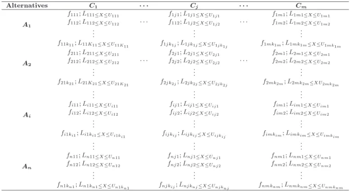
Suppose there are n alternatives Ai(i = 1; 2; ; n) and m criteria Cj(j = 1; 2; ; m). Alternative Ai is evaluated by criterion Cj in the Kij level. The multi-segment problem can be expressed in the matrix format as given in Table 1. Considering this table, fijk is the function of alternative Ai to criterion Cj in the Kth level and x is the variable that depends on an amount of some parameters, such as time, order quantity, and amount of production. For alternative Ai, with respect to criteria Cj, in the kth level, x belongs to [Lijkij; Uijkij]. In the above-mentioned context, the
SAW method with multi-segment decision making is carried out in the following procedure:
Step 1. Consider all intervals, then draw out the lower bounds (Lijkij), and upper bounds (Uijkij) of
intervals from the decision matrix. Sort all of them in ascendant order as: a1; a2; ; ap, where a1 < a2 < < ap.
Step 2. According to the amounts in the pre-vious step, construct the intervals as: [a1; a2]; [a2; a3]; ; [ap 1; ap].
Step 3. Compare all functions of the decision-making matrix under criterion Cj, x 2 [Li; Ui]; i = 1; 2; ; p.
If the intersection between functions exists, then break down intervals [Li; Ui] into several intervals.
The overlapping in every interval is only consid-ered for the functions of one criterion. The functional amounts of alternatives versus each criterion can cross each other. In other words, the values of alternatives versus only one criterion dened as a function are compared with each other (not all criteria for the
Table 1. The multi-segment decision making problem.
Alternatives C1 Cj Cm
A1
f111; L111XU111 f1j1; L1j1XU1j1 f1m1; L1m1XU1m1
f112; L112XU112 f112; L1j2XU1j2 f1m2; L1m2XU1m2
..
. ... ...
f11k11; L11K11XU11K11 f1jk1j; L1jk1jXU1jk1j f1mk1m; L1mk1mXU1mk1m
A2
f211; L211XU211 f2j1; L2j1XU2j1 f2m1; L2m1XU2m1
f212; L212XU212 f2j2; L2j2XU2j2 f2m2; L2m2XU2m2
..
. ... ...
f21k21; L21K21XU21K21 f2jk2j; L2jk2jXU2jk2j f2mk2m; L2mk2mXU2mk2m
..
. ... ...
Ai
fi11; Li11XUi11 fij1; Lij1XUij1 fim1; Lim1XUim1
fi12; Li12XUi12 fij2; Lij2XUij2 fim2; Lim2XUim2
..
. ... ...
fi1ki1; Li1ki1XUi1ki1 fijkij; LijkijXUijkij fimkim; LimkimXUimkim
..
. ... ...
An
fn11; Ln11XUn11 fnj1; Lnj1XUnj1 fnm1; Lnm1XUnm1
fn12; Ln12XUn12 fnj2; Lnj2XUnj2 fnm2; Lnm2XUnm2
..
. ... ...
fn1kn1; Ln1kn1XUn1kn1 fnjkij; LnjknjXUnjknj fnmknm; LnmknmXUnmknm
comparison). Also, the values represented as functions are normalized after the calculations. It is pointed out that in many cases, there is not any overlapping between the two functions.
Suppose that qj intersections points exist as: bi1; bi2; ; biqj:
Construct the (qj+ 1) corresponding intervals as: [Li; bi1]; [bi1; bi2]; [biq 1; biq]; [biq; Ui]:
Like this, construct intervals for other criteria. In addition, we have intervals as:
[L1; b11]; [b11; b12]; ; [b1q1; U1]; ;
[Lj; bj1]; [bj1; bj2]; ; [bjqj; Uj]; ;
[Lp; bp1]; [bp1; bp2]; ; [bpqp; Uq]:
If P0 intervals exist, then nominate them as: [L0
1; U10]; [L02; U20]; ; [L0i; Ui0]; ; [L0p; Up0]:
Step 4. Use the area under the curve of a function as an amount of alternatives versus each criterion in interval [L0
1; U10] as: ijkij =
Z U0
L0 fijkijdx: (4)
Calculate all amounts of the decision matrix by Eq. (4) for all intervals. It is worth noting that the functions
can be dierent in intervals because the decision-making process is done at each level; in other words, each interval (level) has its function and the value of the area under the curve in each level is regarded as an amount of alternatives with respect to criteria in the decision matrix.
Step 5. Calculate the normalized decision matrix. We can obtain the normalized decision matrix denoted by R as:
R = [rijkij];
rijk =
ijk jk
; j 2 B; rijk =
ajk
aijk
; j 2 C; ajk= maxi(aijk); j 2 B;
ajk = mini(aijk); j 2 C: (5) Suppose that B is the set of benet criteria and C is the cost criteria.
Step 6. Consider the dierent importance of each criterion. Then, calculate the nal value of each alternative as:
Pik= m X j=1
rijk:wj; i = 1; 2; ; n;
x 2 [Lijk; Uijk]; (6)
where X is the argument of functions, which demon-strate the amount of variables, such as the amount of primary investment and time. The intervals are broken down according to values of X.
Pik is the nal evaluation value of alternative Ai in the kth level. After the calculation of the nal evaluation value of each alternative, the pair-wise comparison of the preference relationship between the alternatives Ai and Aj can be established.
4. Nomination of some practical functions In this section, we present three commonly-used func-tions that are employed in case studies. Then, the behavior of these functions is investigated. The func-tions may cross each other. Consequently, intercept points can be calculated. The functions are taken into consideration for a single variable. In other words, each function has an independent variable. The value of a variable can generally be changed during the decision making. The variable of each interval has its special function. The variables are recognized as a real variable. Therefore, the functions are presented with real outputs.
4.1. Linear function
Suppose that fijk is the functional amount of alterna-tive Ai to criterion Cj in the kth level. There are two linear functions that are compared with each other as:
fijk = a1x + b1; fi0jk= a2x + b2:
The comparison of the preference relationship between the above functions throughout the interval [lijk; uijk] is as follows:
a) a1 a2, b1 b2 then fijk fi0jk;
b) a1 a2, b1 b2 then fijk fi0jk;
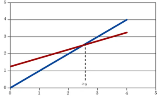
c) a1 a2, b1 b2 or a1 a2, b1 b2 then f1and f2 are intersected in x0= ab21 ba12 as shown in Figure 1. Therefore, the interval [L; U] is broken down into two intervals, [L; x0] and [x0; U].
4.2. Exponential function
Exponential functions are used in many economic problems. This function is introduced in mathematics as:
f(x) = kabx+c;
where k, b and c are stationary coecients.
Figure 1. The comparison of the two linear functions.
fijk = k1ab11x+c1; fi0jk= k2ab22x+c2:
If:
a1; a2 1; k1 k2; a1 a2; b1 b2; c1 c2;
then:
fijk fi0jk:
If:
a1; a2 1; k1 k2; a1 a2; b1 b2; c1 c2;
then:
fijk fi0jk:
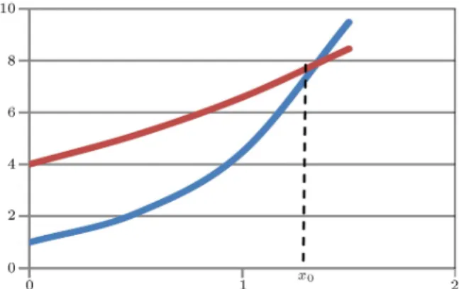
In other words, there is an intersection (x0) between fijk and fi0jk in the interval [lijk uijk] as:
k1ab11x+c1= k2ab22x+c2; therefore:
x0= cb2ln a2 c1ln a1 1ln a1 b2ln a2;
as shown in Figure 2. Also, if a = e, then one has: x0= a 1
1 a2
ln
k1 k2
(b1 b2)
: (7)
4.3. Trigonometric function
The trigonometric function is formed as f = k sin(ax+ b). Let x be an angle that terminates in any quadrant and k, a, b are stationary coecients. This is a periodic function. The trigonometric functions may cross each other; then, intercept points are calculated.
Figure 2. The comparison of the two exponential functions.
Figure 3. The comparison of the two trigonometrical functions.
This function is periodic with period 2
a . For interval [
2; +2], the function is ascending; thus, if k1 k2, a1 a2, b1 b2, then fijk fi0jk.
Now suppose that x 2 [+
2; +32 ]. In this interval, the function can be descending. Therefore, if a1 a2, b1 b2, k1 k2, then fijk fi0jk.
Elsewhere, we have the intersection between func-tions and can draw out the intersection point (x0) from the equation:
k1sin(a1x + b1) = k2sin(a2x + b2); as shown in Figure 3.
5. Application of the proposed method in solving problems
To demonstrate the validity and applicability of the proposed multi-segment SAW method, three illustra-tive cases are provided which are then solved step by step. A summarized description of alternatives and criteria is given. The sensitivity analyses are reported at the end of each case. To further illustrate, the gurations of each case are presented.
5.1. Case 1
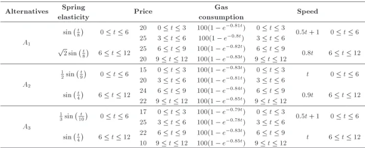
To illustrate the above procedure, the steps of the pro-posed decision-making method are implemented in the application case. In this case study, the performance of three mechanical engines are estimated with respect to four criteria, including spring elasticity, price, amount of gas consumed, and speed, as shown in Figure 4. The aim is to nd the best option among three alternatives. The weights of the criteria are as follows: 0.2, 0.3, 0.1 and 0.4. The performance of each alternative versus criteria is given in Table 2.
The proposed procedure, based on the conceptual model for Case 1, is as follows:
Step 1. Draw out the lower bounds (Lijkij;) and
upper bounds (Uijkij) of intervals from the decision
matrix. Then, sort them in an ascendant order as: 0, 3, 6, 9 and 12.
Step 2. Construct the intervals according to the amount of the previous step as: [03], [36], [69], [912]. Step 3. Compare all functions. Function f112(x) = p
2 sin(t
8) intersects f212(x) = f312(x) = sin(t4), in = 2 = 6:28 2 [6; 9], f141(x) = f341(x) = 0:5t+1 intersect the f241(x) = t, in x = 2 2 [3; 6].
Therefore, break down the intervals [0,3] to [0,2], [2,3] and [6,9] to [6,6.28], [6.28,9]. Then, sort the new intervals as:
[0; 2]; [2; 3]; [3 6]; [6; 6:28]; [6:28; 9]; [9; 12]:
Table 2. The multi-segment decision making matrix of three engines. Alternatives Spring
elasticity Price
Gas
consumption Speed
A1
sin t 8
0 t 6 20 0 t 3 100(1 e 0:81t) 0 t 3 0:5t + 1 0 t 6 25 3 t 6 100(1 e 0:8t) 3 t 6
p 2 sin t
8
6 t 12 25 6 t 9 100(1 e 0:82t) 6 t 9 0:8t 6 t 12 20 9 t 12 100(1 e 0:83t) 9 t 12
A2
1 2sin t9
0 t 6 15 0 t 3 100(1 e 0:83t) 0 t 3 t 0 t 6 20 3 t 6 100(1 e 0:81t) 3 t 6
sin t 4
6 t 12 24 6 t 9 100(1 e 0:84t) 6 t 9 0:9t 6 t 12 22 9 t 12 100(1 e 0:85t) 9 t 12
A3
1 3sin 10t
0 t 6 17 0 t 3 100(1 e 0:79t) 0 t 3 0:5t + 1 0 t 6 25 3 t 6 100(1 e 0:78t) 3 t 6
sin t 4
6 t 12 22 6 t 9 100(1 e 0:83t) 6 t 9 t 6 t 12 10 9 t 12 100(1 e 0:85t) 9 t 12
Table 3. The calculated amount of under curves for three engines.
Duration Alternatives C1 C2 C3 C4
0 t 2
A1 0.25 20 101 3
A2 0.11 15 102.43 2
A3 0.07 17 99.49 3
2 t 3
A1 0.31 20 86.44 2.25
A2 0.135 15 87.08 2.5
A3 0.08 17 85.76 2.25
3 t 6
A1 1.59 25 290.09 9.75
A2 0.715 20 290.84 13.5
A3 0.4 25 289.27 9.75
6 t 6:28
A1 0.27 25 27.81 1.38
A2 0.28 24 27.83 1.55
A3 0.28 22 27.78 1.72
6:28 t 9
A1 3.1 25 271.32 16.6
A2 2.5 24 271.41 18.7
A3 2.5 22 271.22 20.08
9 t 12
A1 4 20 299.92 25.2
A2 1.45 22 299.94 28.35
A3 1.45 10 299.91 31.5
Step 4. Calculate the amounts of area under the curves by Eq. (4) as shown in Table 3. We explicitly demonstrate the calculation of this amount in Ap-pendix A.
Step 5. Calculate the normalized decision matrix by Eq. (5) as shown in Table 4.
Step 6. Calculate the nal evaluation value of alter-native Ai in the kth level. After the calculation of the nal evaluation value for each alternative, the pair-wise
Table 4. The normalized matrix of three engines. Duration Alternatives C1 C2 C3 C4
0 t 2
A1 1 0.75 0.99 1
A2 0.44 1 1 0.67
A3 0.28 0.88 0.97 1
2 t 3
A1 0.23 0.75 0.99 0.9
A2 1 1 1 1
A3 0.06 0.88 0.98 0.9
3 t 6
A1 1 0.8 0.997 0.72
A2 0.45 1 1 1
A3 0.25 0.8 0.995 0.72
6 t 6:28
A1 0.96 0.88 0.999 0.8
A2 1 0.92 1 0.9
A3 1 1 0.998 1
6:28 t 9
A1 1 0.88 1 0.83
A2 0.81 0.92 1 0.93
A3 0.81 1 0.999 1
9 t 12
A1 1 0.50 0.9999 0.8
A2 0.36 0.45 1 0.9
A3 0.36 1 0.9999 1
comparison of the preference relationship between the alternatives Ai, Aj can be established as provided in Table 5. In this case study, the new intervals are sorted as:
[0; 2]; [2; 3]; [3; 6]; [6; 6:28]; [6:28; 9]; [9; 12]:
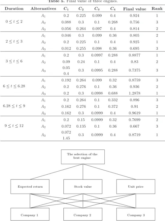
When the performance of the rst machine is compared with the other two machines, as given in Table 5, it is evident that the rst machine has the best perfor-mance value in intervals [0; 2], [3; 6], whereas the third machine has the best performance value in intervals [6; 6:28], [6:28; 9], [9; 12]. Moreover, the second machine
Table 5. Final value of three engines.
Duration Alternatives C1 C2 C3 C4 Final value Rank
0 t 2
A1 0.2 0.225 0.099 0.4 0.924 1
A2 0.088 0.3 0.1 0.268 0.756 3
A3 0.056 0.264 0.097 0.4 0.814 2
2 t 3
A1 0.046 0.3 0.099 0.36 0.805 2
A2 0.2 0.225 0.1 0.4 0.925 1
A3 0.012 0.255 0.098 0.36 0.695 3
3 t 6
A1 0.2 0.3 0.0997 0.288 0.8877 1
A2 0.09 0.24 0.1 0.4 0.83 2
A3 0.05
0.4 0.3 0.0995 0.288 0.7375 3
6 t 6:28
A1 0.192 0.264 0.099 0.32 0.8759 3
A2 0.2 0.276 0.1 0.36 0.936 2
A3 0.2 0.3 0.0998 0.688 1.2878 1
6:28 t 9
A1 0.2 0.264 0.1 0.332 0.896 3
A2 0.162 0.276 0.1 0.372 0.91 2
A3 0.162 0.3 0.0999 0.4 0.9619 1
9 t 12
A1 0.2 0.15 0.0999 0.32 0.7699 2
A2 0.072 0.135 0.1 0.36 0.667 3
A3 0.072
1.45 0.3 0.0999 0.4 0.8719 1
Figure 5. The selection of the best company.
has the best performance value in the interval [2; 3]. Therefore, the preference of alternatives depends on the amount of alternatives in each interval as given in Table 5.
5.2. Case 2
In order to invest in the stock market, it is desired to rank three companies oering their stock, according to the following criteria, as shown in Figure 5:
Expected return for share-holder;
Stock value at the end of maintenance period;
Unit price.
These criteria depend on the amount of initial invest-ment (x). The weights of the criteria are as follows: 0.5, 0.3, and 0.2. The decision matrix is given in Table 6.
The process of the proposed method in Case 2 includes the following steps:
Step 1. Introduce the lower bounds (Lijkij;) and
upper bounds (Uijkij) of intervals and sort them as:
Table 6. The multi-segment decision making matrix of three companies.
Alternatives Expected Return Stock value Unit price
A1
0:1x 0 t 100 xe0 0 t 200 5000-0:2x 0 t 100
0:2x 100 t 1000 xe0 xe1
200 t 600
600 t 1000 5000-0:3x 100 t 1000 A2
0:1x 0 t 200 xe0 0 t 600 6000-0:1x 0 t 100
0:3x 200 t 600 6000-0:2x 100 t 600
0:4x 600 t 1000 xe1 600 t 1000 6000-0:3x 600 t 100
A3 0:2x 0 t 100 xe
0 0 t 200 5000-0:4x 0 t 600
0:3x 100 t 1000 xe0 200 t 1000 5000-0:6x 600 t 1000
Table 7. The calculated amount of under curves for three companies.
Duration Alternatives C1 C2 C3
0 t 100
A1 500 9110.6 499000
A2 500 12298 599500
A3 1000 6749.3 498000
100 t 200
A1 3000 27331.78 495500
A2 1500 36894 597000
A3 4500 20247.88 494000
200 t 600
A1 32000 291539 1952000
A2 48000 393536.5 2368000
A3 48000 393536.5 1936000
600 t 1000
A1 64000 1062437.42 1904000
A2 128000 1062437.42 2304000
A3 96000 787073 1808000
Step 2. Construct the intervals as: [0; 100], [100; 200], [200; 600] and [600; 1000].
Step 3. Compare all functions in all intervals. The functions of this case do not cross each other.
Step 4. Calculate amounts of area under curves by Eq. (4) as given in Table 7.
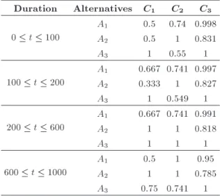
Step 5. Calculate the normalized decision matrix by Eq. (5) as provided in Table 8.
Step 6. Calculate the score of each alternative. The score of each alternative is calculated by Eq. (6) as reported in Table 9. After the calculation of the nal evaluation value for each alternative, alternative Aican be compared with the others as provided in Table 9.
In this case, the new intervals are sorted as: [0; 100]; [100; 200]; [200; 600]; [600; 1000]:
In interval [0; 100], company 1 has the best rank, and companies 2 and 3 have second and third ranks, respectively. In interval [100; 200], the companies are
Table 8. The normalized matrix of three companies. Duration Alternatives C1 C2 C3
0 t 100
A1 0.5 0.74 0.998
A2 0.5 1 0.831
A3 1 0.55 1
100 t 200
A1 0.667 0.741 0.997
A2 0.333 1 0.827
A3 1 0.549 1
200 t 600
A1 0.667 0.741 0.991
A2 1 1 0.818
A3 1 1 1
600 t 1000
A1 0.5 1 0.95
A2 1 1 0.785
A3 0.75 0.741 1
ranked as A2 > A3 > A1. In interval [200; 600], they are ranked as A3> A2> A1. Moreover, companies are ranked as A3> A1 > A2 in the interval [600; 1000] as given in Table 9.
5.3. Case 3
It is desired to evaluate three nancial institutes. They receive an initial investment (t) from customers and return their investments and the cost of money (the interest rate). Now, the investor wants to select one from among these three nancial rms. To do so, it is required to rank them according to the following criteria as shown in Figure 6:
Protability index;
The criterion of net present value; The amount of amortization.
The weights of the criteria are as follows: 0.4, 0.4, and 0.2. The decision matrix is given in Table 10.
The step by step problem-solving process is pro-posed for the third case as follows:
Step 1. Calculate lower bounds (Lijkij;) and upper
bounds (Uijkij) of intervals, and the results are as
Table 9. Final value of three companies.
Duration Alternatives C1 C2 C3 Final value Rank
0 t 100
A1 0.25 0.222 0.2 0.672 3
A2 0.25 0.3 0.166 0.716 2
A3 0.5 0.165 0.2 0.865 1
100 t 200
A1 0.334 0.222 0.199 0.755 2
A2 0.167 0.3 0.165 0.632 3
A3 0.5 0.165 0.2 0.865 1
200 t 600
A1 0.334 0.222 0.198 0.754 3
A2 0.5 0.3 0.164 0.964 2
A3 0.5 0.3 0.2 1 1
600 t 1000
A1 0.25 0.3 0.19 0.74 3
A2 0.5 0.3 0.157 0.957 1
A3 0.375 0.222 0.2 0.797 2
Table 10. The multi-segment decision making matrix of three institutes.
Alternatives Protability Index Net present Value Amortization
A1 (1:2)
t 1 t 10 (3)t (2)t 1 t 10 0:2t 1 t 10
(1:4)t 10 t 20 (4)t (2)t 10 t 20 0:3t + 3
2 10 t 20
A2 (1:2)
t 1 t 10 (3)t (2)t 1 t 10 0:1t 1 t 10
(1:5)t 10 t 30 (4)t (2)t 10 t 30 0:4t 10 t 30
A3
(1:1)t
(1:3)t
1 t 10 10 t 20 (4)
t (2)t 1 t 20 0:4t 1 t 20
(1:4)t 20 t 30 2((4)t (2)t) 20 t 30 0:5t 20 t 30
Figure 6. The selection of the best institute.
Step 2. Obtain the intervals obtained as: [1; 10], [10; 15], [15; 20] and [20; 30].
Step 3. Compare all functions. Function f132(x) = 0:3t +3
2 intersects f331(x) = 0:4t. In x = 15 2 [10; 20]. Therefore, break down the interval [10; 20] to [10; 15] and [15; 20]. Then, sort the new intervals as: [1; 10],
[10; 15], [15 20] and [20; 30].
Step 4. Use Eq. (4) for calculating the amount of area under curves as given in Table 11.
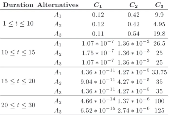
Step 5. Calculate the normalized decision matrix by Eq. (5) as provided in Table 12.
Table 11. The calculated amount of under curves for three institutes.
Duration Alternatives C1 C2 C3
1 t 10
A1 0.12 0.42 9.9
A2 0.12 0.42 4.95
A3 0.11 0.54 19.8
10 t 15
A1 1:07 10 7 1:36 10 3 26.5
A2 1:75 10 7 1:36 10 3 25
A3 1:07 10 7 1:36 10 3 25
15 t 20
A1 4:36 10 114:27 10 533.75
A2 9:04 10 114:27 10 5 35
A3 4:36 10 114:27 10 5 35
20 t 30 A2 4:66 10 141:37 10 6 100 A3 6:52 10 152:74 10 6 125
Table 12. The normalized matrix of three institutes. Duration Alternatives C1 C2 C3
1 t 10
A1 1 0.78 0.5
A2 1 0.78 1
A3 0.92 1 0.25
10 t 15
A1 0.611 1 0.94
A2 1 1 1
A3 0.611 1 1
15 t 20 AA12 0.481 11 0.961
A3 0.48 1 0.96
20 t 30 A2 1 0.5 1
A3 0.14 1 0.8
Step 6. Calculate the nal evaluation value of each alternative. After calculation of the nal evaluation value of each alternative, the pair-wise comparison of the preference relationship between the alternatives can be established as given in Table 13. In this case, the new intervals are sorted as [1; 10], [10; 15], [15; 20], and [20; 30] as given in Table 13.
The institutes are ranked in each interval. The
preferences of these institutes are presented as: [1; 10]; A3> A1> A2;
[10; 15]; A3> A1> A2; [15; 20]; A2> A1> A3; [20; 30]; A2> A3; 6. Result and discussion
In our proposed decision method, a multi-segment decision matrix is employed to determine the preference of alternatives in multi-segment problems, which can be easily solved by this method step by step. This research has conducted a performance analysis on three case studies using a multi-segment MCDM approach. In the rst case study, there are four criteria for ranking the alternatives. The rst criterion is the amount of spring elasticity. The rate of elasticity
is indicated by the following relation:
Y = a sin(!t + 0); (8)
where t is a variable referring to the time of receiving the customer order. The unit of time in this problem is a month. The amplitude A of a wave is the magnitude of the maximum displacement of the individual parti-cles from their equilibrium position. ! = 2=T = 2f is the angular frequency of the wave. ? is called the phase constant. 0 is the initial phase of the vibrating particle (i.e., phase t = 0). The term !t + 0 is known as the phase of the vibrating particle.
The level of elasticity is regarded as a positive criterion, that is, more elasticity is favored. Production companies produce dierent springs depending on the changes of conditions, like the climate condition. The elasticity of springs produced in the rst half of the year vary from those produced in the second half as depicted in Figure 7. The elasticity of the springs produced in
Table 13. Final value of three institutes.
Duration Alternatives C1 C2 C3 Final value Rank
1 t 10
A1 0.4 0.312 0.1 0.812 3
A2 0.4 0.312 0.2 0.912 1
A3 0.368 0.4 0.05 0.818 2
10 t 15
A1 0.24 0.4 0.188 0.828 3
A2 0.4 0.4 0.2 1 1
A3 0.24 0.4 0.2 0.84 2
15 t 20
A1 0.192 0.4 0.2 0.792 2
A2 0.4 0.4 0.192 0.992 1
A3 0.192 0.4 0.192 0.784 3
20 t 30 A2 0.4 0.2 0.2 0.8 1
Figure 7. The amount of engines versus spring's elasticity.
the rst half of the year for every company is obtained by the following relation:
A1: x = sin 8t ! =810; T = 16;
A2: x = 12sin 9t ! =910; T = 18;
A3: x = 13sin 10t ! =1010; T = 20:
All three above-mentioned functions are ascending in the interval [0; 6]. So, the producer increases the elasticity of the produced springs through time. As indicated in Figure 7, the three functions do not cross each other in the rst half of the year.
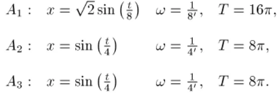
The elasticity of springs produced in the second half of the year is calculated by following relations:
A1: x =p2 sin t8 ! = 810; T = 16;
A2: x = sin 4t ! = 410; T = 8;
A3: x = sin 4t ! = 410; T = 8:
As shown in Figure 7, the functions cross at the point t = 2 = 6:28. Thus, the interval in [0; 6] is divided into two intervals in [6; 6:28] and [6:28; 12].
The second criterion of the ranking is the price of the produced engines. The engines are priced by the companies every three months. So, the price of products is xed to the end of each session according to Table 14.
Since this criterion is negative, the less the value assigned to the alternatives, the better the given alternative. In this way;
0 t 3 A2> A3> A1; 3 t 6 A2> A3= A1; 6 t 9 A3> A2> A1; 9 t 12 A3> A1> A2:
The third criterion is the amount of gas consumed.
Table 14. The amount of engines with respect to price. Duration Alternatives Price
0 t 3
A1 20
A2 15
A3 17
0 t 3
A1 25
A2 20
A3 25
0 t 3 AA12 2524
A3 22
0 t 3
A1 20
A2 22
A3 10
The amount of existing gas in time t is shown by the following function:
y = y0e kt; (9)
where k is the coecient of daily usage, y0 is the amount of initial gas which equals 100 liters. The fuel tank is lled daily.
The engines produced in companies 1, 2 and 3 have dierent gas consumption rates in every season. In all companies, the amount of gas consumed in the second quarter of the year (summer) is less than in other seasons and in the fourth quarter (winter) is more than other seasons. As shown in Figure 8, this criterion is a negative one, that is, the less the gas consumption rate, the better.
The fourth criterion is the speed. This is a positive criterion, so the more the speed, the better. In the rst half of the year, the producing companies produce engines with dierent speed capabilities from the second half as follows:
0 t 6; 8 > < > :
A1: v = 0:5t + 1 A2: v = t A3: 0:5t + 1
Figure 8. The amount of engines versus the amount of gas consumed.
Figure 9. The amount of engines versus the speed.
6 t 12; 8 > < > :
A1: v = 0:8t A2: v = 0:9t A3: t
As shown in Figure 9, the functions cross each other at point t = 2. Thus, the interval [0; 3] is divided into two intervals of [0; 2] and [2; 3]. This means that in interval [0; 2], the engines of company 1 are better than those of the other company, while the engines of company 2 have more speed in the interval of [2; 3] as shown in Figure 9.
In the second case study, the rst criterion is the expected turnover by the stockholders; the more the turnover, the better. Functions regarded as the expected turnover are ascending, that is, the more the amount of initial investment, the more the amount of turnover expected. In company A1, if the investment is in interval [0; 100], the expected turnover is 0.1 of the inventory, whereas if the investment is in interval [100; 1000], the amount of turnover expected can be 0.2 of the inventory. Also, for company A2, the amount of turnover expected is at three levels, and at two levels for company A3, which are presented in Figure 10.
The second criterion is the stock value at the end of the maintenance period. It is a positive criterion. The functions assigned to the alternative in this criterion are ascending. Like the rst criterion, the value of stock at the end of the period is proportionate to the initial investment. The future value of stock for companies A1, A2 and A3 is presented at two levels. Like Figure 11, there is no overlapping of functions.
The third criterion is the price of each stock unit. Higher prices are not suitable to be invested. The func-tions assigned to this criterion are descending. Thus, the companies increase the discounts applied to stock prices proportionate to the number of units purchased, in order to encourage companies for the investment. For instance, if the amount of the investment is between 0 and 100 for company A1, the investors will have a 0.2 discount. If the purchased stock units are between 100 and 1000, the amount of discount will be 0.3. Also, companies A2 and A3 have their regulations in
Figure 10. The values of companies versus an expected return on share-holder.
Figure 11. The values of companies versus the stock value at the end of maintenance period.
Figure 12. The values of companies versus an amount of price.
dierent levels. As depicted in Figure 12, there is no overlapping of functions in the interval of 0 and 1000 in the third criteria. As observed in the process of solving the second case, the ranking is done in every interval.
In the third case study, the rst criterion of the decision-making process is the protability. The protability varies according to the initial investment in dierent institutes. In institute A, if initial in-vestment is 1 to 10 units, the protability can equal (1:2)t, whereas, if the initial investment (t) is 10 to
Figure 13. The values of institutes versus protability index.
Figure 14. The values of institutes versus the criterion of net present value.
20, the protability can be (1:4)t to encourage more investment. The maximum amount of investment in institute A1 is 20 units, while in institutes A2 and A3 it is possible to invest up to 30 units. The functions of this criterion do not cross each other as shown in Figure 13.
The second criterion is the net present value. This is a positive criterion; in other words, the more the net present value, the better. Like Figure 14, there is no overlapping of functions.
The third criterion is the amount of amortization. Since this criterion is a negative one, the less the value assigned to the alternatives, the better the given alternative. The functions cross each other at point t = 15. Thus, interval [10; 20] is divided into two intervals [10; 15] and [15; 20] as shown in Figure 15.
Based on the results of the analysis, some essential ndings are discussed as follows. Because the SAW method is very easy and the proposed method is provided step by step, the computation process is simple and straightforward. Moreover, the DM can nd the best alternative in each interval. In some cases, an overlapping of the curves of the functions may exist. Hence, the preference of alternatives may be changed in each interval. Considering this concept, the new method is proposed as a logical mathematical tool to help the DM in order to make the best decision.
Figure 15. The values of institutes versus the amount of amortization.
During this multi-segment approach, one parameter alone is not taken into consideration to deal with the complex decision problems. Many parameters can be introduced, such as time, order quantity, and amount of production. This method can assist the DM when the order quantity of alternatives is not exactly provided, and then the bounds of the order quantity are assigned as an interval. In this method, the values of alternatives with respect to criteria are transformed into the dimensionless value. Thus, the nal value of alternatives can be calculated where the criteria are presented with dierent dimensions. For example, in the rst case study, three mechanical engines are estimated with respect to four criteria, including spring elasticity, price, amount of gas consumed, and speed. When comparing the performance of the rst machine with the other two machines, it can be observed that the rst machine has the best performance value in intervals [0; 2] and [3; 6], whereas the third machine has the best performance value in intervals [6; 6:28], [6:28; 9] and [9; 12]. Moreover, the second machine has the best performance value in interval [2; 3]. Hence, the preference of alternatives depends on the amount of alternatives in each interval. In the second and third cases, by considering the preference criteria, the rankings of alternatives are dierent in each interval where each interval has the corresponding ranking. This leads to a competitive advantage because other methods cannot consider these factors and only present the preference without considering environmental con-ditions.
As mentioned in Section 1, all response spaces are considered. The presented method is a decision-making method. The main dierence from other methods is that the proposed decision-making method can change under dierent conditions, according to the complexity of the decision problems in a real-world situation. The previous methods have provided only one ranking throughout the decision-making process
and the decision matrix has a xed value, whereas in this method, besides changing the decision-matrix in dierent levels, the values can be properly regarded as a function. For example, in the rst case, instead of presenting one ranking in general ([0; 12]), the decision-making process is done by considering the values of functions related to each alternative in each of the corresponding intervals (i.e., [0; 2], [2; 3], [3; 6], [6; 6:28], [6:28; 9] and [9; 12]).
7. Conclusion
In this paper, a new SAW method was proposed to solve problems in which an amount of alternatives, with respect to criteria, is presented in several levels. The proposed method led to preference alternatives in multi-segment problems which can be easily solved by the step by step method. Considering the fact that in real-world situations, the value of alternatives is not stationary under every condition, the proposed method can be applied to deal with problems wherein the data of the decision matrix is introduced as a functional amount, and can be dependent on some parameters at every level. Therefore, the functional amounts were employed and compared to rank the alternatives in real-life situations. The area under curves was used in order to calculate the elements of the matrix. Because the assessment value changed under dierent conditions for the complex decision problem, this method has high accuracy in determining the preference of all options. Moreover, this method can help the decision maker when the order quantity is not determinable and the bounds of the order quantity are assigned as an interval. Hence, this method is applied to a greater number of issues in order to deal with real-world decision problems under multiple criteria. Finally, to show the validity and applicability of the proposed SAW method, based on a multi-segment decision making matrix, three illustrative cases were provided. Then, the sensitivity analysis was described in detail. The weight of criteria was changeless during the problem-solving, whereas the weight of criteria can be represented in several segments. Also, the weight can be represented as a function of some parameters. This subject is recommended for further research in discrete decision-making problems.
References
1. Pomerol, J.C. and Romero, S.B. \Multicriterion de-cision in management", Principles and Practice, C. James, Trans., 1st Edn., Kluwer Academic Publishers, Norwell (from French) (2000).
2. Tor, F., ZanjiraniFarahani, S. and Rezapour, S. \Fuzzy AHP to determine the relative weights of evaluation criteria and fuzzy TOPSIS to rank the
alternatives", Applied Soft Computing, 10, pp. 520-528 (2010).
3. Hwang, C.L. and Yoon, K., Multiple Attribute Decision Making - Method and Applications, A State-of-the-Art Survey, Springer-Verlag, New York (1981).
4. Virvou, M. and Kabassi, K. \Evaluating an intelligent graphical user interface by comparison with human experts", Knowledge-Based Systems, 17, pp. 31-37 (2004).
5. Tecle, A. and Duckstein, L. \Selecting a multi criterion decision making technique for watershed resources management", Water Resources Bulletin, 28(1), pp. 129-140 (1992).
6. MacCrimmon, K.R. \Decision making among mul-tiple attribute alternatives", A Survey and Consol-idated Approach, RAND Memorandum, RM-4823-ARPA (1968).
7. Manokaran, E., Subhashini, S., Senthilvel, S., Muru-ganandham, R. and Ravichandran, K. \Application of multi criteria decision making tools and validation with optimization technique", Case Study Using TOPSIS, ANN & SAW. IJMBS, 1(3), pp. 2231-2463 (2011). 8. Afshari, A., Mojahed, M. and Yusu, R.-M.
\Sim-ple additive weighting approach to personnel selec-tion problem", Internaselec-tional Journal of Innovaselec-tion, Management and Technology, 1(5), ISSN: 2010-0248 (2010).
9. Kabassi, K. and Virvou, M. \Personalised adult e-training on computer use based on multiple attribute decision making", Interacting with Computers, 16, pp. 115-132 (2004).
10. Chou, S.Y., Chang, Y.H. and Shen, C.Y. \A fuzzy simple additive weighting system under group decision-making for facility location selection with objec-tive/subjective attributes", European Journal of Op-erational Research, 189, pp. 132-145 (2008).
11. Kotler, P. and Keller, K.L., Marketing Management (12e), NJ, Prentice-Hall (2006).
12. Liao, C-N. \Formulating the multi-segment goal pro-gramming", Computers & Industrial Engineering, 56, pp. 138-141 (2009).
13. Chen, S.-P. and Ho, Y.-H. \Analysis of the news-boy problem with fuzzy demands and incremental discounts", International Journal of Production Eco-nomics, 129(1), pp. 169-177 (2011).
14. Ahi, A., Aryanezhad, M.-B., Ashtiani, B. and Makui, A. \A novel approach to determine cell formation, intracellular machine layout and cell layout in the CMS problem based on TOPSIS method", Computers & Operations Research, 36, pp. 1478-1496 (2009).
Appendix
Here, the calculation style is described for the amount of area under curve for alternative A1 versus criterion
C1 in the rst level. Like this, other amounts can be calculated. According to Table 2, we have:
f(t)= sin
t 8
; a111=
Z 2 0 sin
t
8dt = 0:25; 0 t: Biographies
Meghdad Salimi received a BS degree from the Department of Applied Mathematics at Amirkabir University of Technology, Tehran, Iran, and is cur-rently an MS student in the Department of Industrial Engineering at Islamic Azad University, Qazvin, Iran. His research interests include multi-criteria decision making and applied operations research.
Behnam Vahdani obtained BS, MS and PhD degrees from the Department of Industrial Engineering at Tehran University, Iran, and is a member of Iran's Na-tional Elite Foundation. His current research interests include: Supply chain network design, facility location and design, logistics planning and scheduling, multi-criteria decision making, uncertain programming, arti-cial neural networks, meta-heuristics algorithms and operations research applications. He has published
several papers and book chapters in the aforementioned areas.
Seyed Meysam Mousavi received a PhD degree from the Department of Industrial Engineering at Tehran University, Iran, and is currently a member of Iran's National Elite Foundation and Young Researches Club. His main research interests include: cross-docking systems planning, project risk management, project selection and scheduling, engineering optimization un-der uncertainty, facilities planning and design, mul-tiple criteria decision making under uncertainty, soft computing, articial intelligence, and meta-heuristics algorithms. He has published several papers and book chapters in reputable journals and international conference proceedings.
Reza Tavakkoli-Moghaddam received his MS de-gree in Industrial Engineering from Melbourne Univer-sity, Australia, and his PhD degree from Swinburne University of Technology, UK. He is currently Pro-fessor of Industrial Engineering at Tehran University, Iran. His research interests include facility layouts and location design, cellular manufacturing systems, sequencing and scheduling, and using meta-heuristics for combinatorial optimization problems. He is the author of over 100 journal papers and 150 papers in conference proceedings.