ISSN: 2252-8938, DOI: 10.11591/ijai.v8.i2.pp190-196 190
Sensitivity analysis of a species conserving genetic algorithm's
parameters for addressing the niche radius problem
Michael Scott BrownUniversity of Maryland University College, Adelphi, MD 20774, USA
Article Info ABSTRACT
Article history: Received Feb 29, 2019 Revised Apr 20, 2019 Accepted Apr 1, 2019
Niche Genetic Algorithms (NGA) are a special category of Genetic Algorithms (GA) that solve problems with multiple optima. These algorithms preserve genetic diversity and prevent the GA from converging on a single optima. Many NGAs suffer from the Niche Radius Problem (NRP), which is the problem of correctly setting a radius parameter for optimal results. While the selection of the radius value has been widely researched, the effects of other GA parameters on genetic diversity is not well known. This research is a parameter sensitivity analysis on the other parameters in a GA, namely mutation rate, number of individuals and number of generations.
Keywords: Genetic Algorithm Niche Radius Problem Sensitivity Analysis
Copyright © 2019 Institute of Advanced Engineering and Science. All rights reserved. Corresponding Author:
Michael Scott Brown,
University of Maryland University College, Adelphi, MD 20774, USA.
Email: [email protected]
1. INTRODUCTION
Background
Niche Genetic Algorithms (NGAs) have been shown to be very successful solving optimization problems in multi-optima domains. But many of these algorithms incorporate a radius parameter that when set poorly produce less than desirable results. This is known as the Niche Radius Problem (NRP). Some algorithms claim to address the NRP. But, the potential of algorithms that suffer from NRP warrants additional research in this area.
The Problem
Much research has been published concerning the role that the radius parameter plays in NGAs. For Fitness Sharing NGAs some research indicates that population size plays a role in genetic diversity [1]. Little research has looked at the parameters used in NGAs, namely the population size, number of individuals per generation and mutation rate. This research conducts a parameter sensitivity analysis on these other parameters using a popular NGA called the Species Conserving Genetic Algorithm [2].
The Proposed Solution
This research will begin to address how NGA parameters affect their ability to locate optima. Learning about the effects of parameters on the NRP is important for many reasons. When doing research in NGAs this research could be used for selecting parameter values. As we continue to address the NRP, NGAs that suffer from NRP will be more useful. Continued research into the NRP has many benefits.
2. PROPOSED METHOD 2.1. Niche radius problem
GAs are well suited for finding optima in problems that only contain a single optima [3]. In multi-optima problems traditional GAs may converge on a local optima and miss the global optima. A special subset of GAs, called Niche Genetic Algorithms (NGAs), is specifically designed to preserve optima [4-5]. But a number of these algorithms have a radius parameter and determining a good value for the radius can be problematic. The Niche Radius Problem (NRP) is the inability to select a good radius value for radius based NGAs without knowing the distance between optima [6]. The only effective way to determine the distance between optima is to know where the optima are located. But if we knew the location of the optima there would be no need to run the NGA, since optima location is the purpose of the NGA. This creates a paradox in that NGAs can locate the optima assuming that radius is set correctly, which requires knowledge of where the optima are located.
NGAs are good at solving multi-optima problems because they preserve areas of the domain and prevent global convergence. By preserving genetic diversity all of the optima can be located. There are NGAs that address the NRP. CMA-ES [7-9], GAS [10-11], DSGA [12], Fan, Sheng and Chen [13] and Asymmetric Sharing [14-15] all address this problem to some degree. But it is important to continue to do research on the NRP because solving it will provide us with more useful NGA algorithms. One such algorithm that could benefit from more research on the NRP is the Species Conserving Genetic Algorithm (SCGA) [2]. SCGA suffers from poor performance when the radius is incorrectly selected [2]. 2.2. Species conserving genetic algorithm
SCGA is an NGA that attempts to conserve areas of the domain [2]. The population of all GAs is under two distinct pressures. There is an explorative pressure found in mutation. Mutation allows the GA to explore new areas of the domain. There is also an exploitative pressure, which is found in selection. This pressure allows the GA to capitalize on fit areas of the domain. Over time the exploitative pressures overcome the explorative pressures. SCGA identifies unique areas of the domain and prevents the exploitative forces from eliminating them until they can be explored [2]. Traditional GAs iteratively performs three operations: selection, crossover and mutation [17, 3]. SCGA enhances the GA by adding two additional operations: seed selection and seed conservation yielding pseudo code as follows [2].
Initial population
Begin loop until some terminate condition Seed selection
Selection Crossover Mutation
Seed conservation End loop
The seed selection operation has a radius parameter, r [2]. It evaluates each individual in the current population from the most fit to the least fit. For each individual that it evaluates it checks to see if there is another seed within distance r. If no seed exists within r then the individual is marked as a seed. If there is a seed within r then the individual is not a seed. Seeds are locally strong individuals within the radius r. Seed conservation ensures that seeds are represented in the next generation [2]. Each seed will replace an individual in the next generation. The operation begins by evaluating the individuals in the next generation within distance r of the seed. If individuals exist in this area of the domain the seed replaces the weakest individual in this area of the domain. If the next generation contains no individuals within this area then the seed replaces the globally weakest individual in the next generation. SCGA is a novel algorithm that preserves locally strong individuals. This preserves their genetic traits and allows them to attempt to find local optima [2].
3. RESEARCH METHOD
3.1. Sensitivity analysis
Sensitivity Analysis is the study of the effect that parameter values have on mathematical models [18]. Sensitivity Analysis can help determine which parameters justify further investigation and which parameters correlate with the output. There are a variety of methods to perform sensitivity analysis. One popular method is the One at a time (OAT) method. In OAT we begin with a baseline set of parameter values. Parameter values are varied one at a time while measuring the change in the output. In this research the following parameter values were selected for the base case. The population size, N, was set to 100.
The gene mutation rate, M, was set to 0.01. The number of generations, G, was set to 200. The radius, r, was set to 0.1. All of these values were used in prior research on SCGA [2, 12]. The variation of the parameter values will be ±10%, ±20% and ±40% compared to the base case values. Since we want to preserve genetic diversity we will measure the standard deviation of the domains values in the final generation with the goal of this being high. A low standard deviation would indicate global convergence. We will also measure the average fitness of the final generation.
3.2. Benchmarks
There are a number of widely used benchmarks for multimodal optimization problems. Bernier [16] generalized many of these functions into equation 1.
𝑓(𝑥) = 𝑅𝑐−𝑐𝑥2sin (𝑘𝜋𝑥6 𝑝) (1)
Different values for R, c, p and k will yield different functions. The value of c determines the rate of decay of the oscillation. Normally k determines the number of optima and R determines the range value of the optima. Some form of this equation has been used in many research papers on NGAs [19-21, 1].
The benchmarks used in this research are shown in equations F1 through F3. All of these problems are maximization problems where the value of x is between 0 and 1 inclusive. All are forms of (1) and have been used in other research.
𝑓(𝑥) = sin (5𝜋𝑥6 ) (F1)
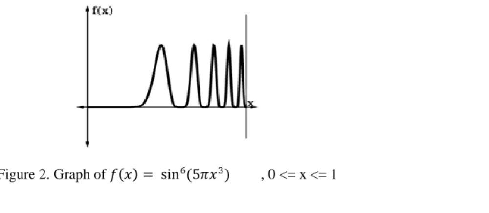
𝑓(𝑥) = sin (5𝜋𝑥6 3) (F2)
𝑓(𝑥) = sin (10𝜋𝑥6 2) (F3)
These specific functions have also been used in other research as benchmarks [16, 12]. Function 1 is a sine function with optima spaced evenly throughout the domain all with the same range values. When x is between 0 and 1 the function has 5 optima. A graph of the function can be seen in Figure 1.
Figure 1. Graph of (𝑥) = sin (5𝜋𝑥6 ) , 0 <= x <= 1
Function 2 also has 5 optima when x ranges between 0 and 1. However, unlike F1 that has optima evenly spaced within the domain, F2 optima are increasingly closer together as x increases. Figure 2 shows a graph of F2.
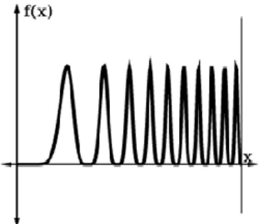
Function 3 has 10 optima when x ranges between 0 and 1. Similar to F2, these optima appear closer together as x increases. Figure 3 shows a graph of F3.
Figure 3. Graph of 𝑓(𝑥) = sin (10𝜋𝑥6 2), 0 <= x <= 1
3.3. Experiment
In this experiment a number of test cases were executed. The base case of N = 100, G = 200 and M = 0.01 was executed and is used for comparison against all of the base cases. Each variation of ±10%, ±20% and ±40% for each parameter was also executed. The mutation rate is a gene mutation rate. It is evaluated on each gene of each individual in the new generation. A mutation rate of 0.01 would mean that 1% of genes are selected for mutation. This does allow for the possibility that multiple genes in an individual could be mutated. The modeling of domain values as individual uses the method of evenly dividing the domain [22]. The range of domain values has an upper bound (UB) of 1 and the lower bound (LB) of 0. If we assume that the chromosomes are bn-1bn … b1b0, the following equations shows the representation for the domain value x. Function 2 shows the equation for converting individuals to domain values.
𝑥 = 𝐿𝐵 +∑𝑛−1𝑖=0𝑏𝑖2𝑛
2𝑛−1 (𝑈𝐵 − 𝐿𝐵) (2)
This equation makes an individual of all 0's be the LB and an individual of all 1's be the UB. All domain values in between are divided evenly based upon the number of chromosomes in an individual. In this research 30 chromosomes were used. As stated early genetic diversity is measured through larger values of the standard deviation of the domain values in the final generation. Additionally, this research documents the average fitness of the final generation. This is included because it is not advantageous to increase genetic diversity at the expense of fitness. This would mean that the GA individuals have not located the optima. Since GAs are non-deterministic results may vary for each execution of the algorithm. For each combination of parameters the SCGA was executed 20 times and all results were averaged. Standard deviation is really the average standard deviation of the 20 runs. A few computed values are also provided. The difference as a percent of standard deviation is calculated for each parameter set compared to the base case. The difference as a percent of average fitness is also calculated. This makes it easy to compare a parameter set to the base case. Finally, the Student T-Test is performed [23]. The T-Test compares the standard deviation of the 20 test cases for the base case to each set of parameters. The p value is determined. The p value threshold of 0.05 is used to determine statistical significance.
4. RESULTS AND DISCUSSION
Experiment results are documented in Tables 1 through 9. Tables 1 through 3 contain results for function F1. Tables 4 through 6 contain results for function F2. Tables 7 through 9 contain results for function F3. Each table is dedicated to the results from changing one parameter. In each table the first row is the base case followed by a row for each parameter values changed. Column SD is the average of standard deviations of the domain values of the final generation. Ideally, we would like this to be large showing genetic diversity. Column AF is the average fitness of the final generation. The next two columns show the difference as a percent of the base case to the parameter set values. The final column p is the p value from the T-Test. Using the value of p equal to 0.05 as a threshold for statistical significance, this research produces very mixed results. For function F1 the cases of N = 60, M = 0.008 and M = 0.006 produce statistically significant results. M = 0.009 comes very close with a p value of 0.052. For function F2 the cases of G = 240
and G = 160 produce statistically significant results. For F3 only G = 120 produce statistically significant results. When performing a parameter sensitivity analysis statistically significant results indicate a correlation between the parameter and genetic diversity.
Table 1. Results of varying N for F1 N SD AF ∆𝑆𝐷 ∆𝐴𝐹 p
100 0.1889 0.9887 N/A N/A N/A
110 0.1499 0.9666 -21% -2% 0.67
120 0.2804 0.9516 48% -4% 0.7
140 0.1983 0.9311 5% -6% 0.86
90 0.1690 0.9679 -11% -2% 0.12
80 0.2451 0.9723 30% -2% 0.37
60 0.2656 0.9661 41% -2% 0.039
Table 2. Results of varying G for F1 G SD AF ∆𝑆𝐷 ∆𝐴𝐹 p
200 0.1889 0.9887 N/A N/A N/A
220 0.2611 0.9343 38% -6% 0.92
240 0.2524 0.9428 34% -5% 0.59
280 0.2788 0.9544 48% -3% 0.93
180 0.2225 0.9812 18% -1% 0.55
160 0.1958 0.9428 4% -5% 0.14
120 0.2606 0.9569 38% -3% 0.5
Table 3. Results of varying M for F1 M SD AF ∆𝑆𝐷 ∆𝐴𝐹 p
0.01 0.1889 0.9887 N/A N/A N/A
0.011 0.1099 0.9839 -42% 0% 0.87
0.012 0.1738 0.9861 -8% 0% 0.88
0.014 0.1457 0.9650 -23% -2% 0.24
0.009 0.1216 0.9889 -36% 0% 0.052
0.008 0.2350 0.9758 24% -1% 0.032
0.006 0.1692 0.9757 -10% -1% 0.027
Table 4. Results of varying N for F2 N SD AF ∆𝑆𝐷 ∆𝐴𝐹 p
100 0.1395 0.9842 N/A N/A N/A
110 0.2363 0.9905 69% 1% 0.17
120 0.1190 0.9912 -15% 1% 0.46
140 0.2200 0.9808 58% 0% 0.88
90 0.0943 0.9888 -32% 0% 0.19
80 0.0669 0.9869 -52% 0% 0.31
60 0.1747 0.9830 25% 0% 0.98
Table 5. Results of varying G for F2 G SD AF ∆𝑆𝐷 ∆𝐴𝐹 p
200 0.1394528 0.9841 N/A N/A N/A
220 0.0693409 0.9897 -50% 1% 0.99
240 0.2545786 0.9870 83% 0% 0.047
280 0.1986731 0.9893 42% 1% 0.44
180 0.0700884 0.9892 -50% 1% 0.63
160 0.1529781 0.9888 10% 0% 0.032
120 0.1400206 0.9857 0% 0% 0.40
Table 6. Results of varying M for F2 M SD AF ∆𝑆𝐷 ∆𝐴𝐹 p
0.01 0.1395 0.9842 N/A N/A N/A
0.011 0.1860 0.9470 33% -4% 0.41
0.012 0.0945 0.9878 -32% 0% 0.26
0.014 0.1580 0.9788 13% -1% 0.22
0.009 0.0717 0.9897 -49% 1% 0.57
0.008 0.1042 0.9890 -25% 0% 0.87
0.006 0.0976 0.9836 -30% 0% 0.85
Table 7. Results of varying N for F3 N SD AF ∆𝑆𝐷 ∆𝐴𝐹 p
100 0.1909 0.9866 N/A N/A N/A
110 0.1481 0.9683 -22% -2% 0.46
120 0.1833 0.9608 -4% -3% 0.29
140 0.1586 0.9670 -17% -2% 0.77
90 0.2381 0.9636 25% -2% 0.29
80 0.0978 0.9840 -49% 0% 0.88
60 0.0625 0.9833 -67% 0% 0.07
Table 8. Results of varying G for F3 G SD AF ∆𝑆𝐷 ∆𝐴𝐹 p
200 0.1909 0.9866 N/A N/A N/A
220 0.1345 0.9830 -30% 0% 0.52
240 0.3717 0.9389 95% -5% 0.46
280 0.1264 0.9800 -34% 0% 0.91
180 0.1841 0.9585 -4% -3% 0.10
160 0.1157 0.9729 -39% -1% 0.26
120 0.2286 0.9479 20% -4% 0.02
Table 9. Results of varying M for F3 M SD AF ∆𝑆𝐷 ∆𝐴𝐹 p
0.01 0.1909 0.9866 N/A N/A N/A
0.011 0.2711 0.9651 42% -2% 0.12
0.012 0.3013 0.9610 58% -3% 0.27
0.014 0.1288 0.9952 -33% 1% 0.22
0.009 0.2700 0.9332 41% -5% 0.24
0.008 0.1501 0.9848 -21% 0% 0.29
0.006 0.0540 0.9900 -72% 0% 0.96
5. CONCLUSION
This research only begins to examine the relationship between genetic diversity and NGA parameters. More research needs to be done. This gives rise to numerous areas of additional research. This research only used one NGA algorithm, SCGA, but there are other NGAs that could benefit from this research. An algorithm doesn't necessarily need to use the term radius to be a candidate for further research. The Fitness Sharing algorithm [19] also suffers from the NRP [10]. Any of these types of algorithms would
make a good subject for future research.One-at-a-time is not the only sensitivity analysis method. There are many others. Differential Sensitivity Analysis develops sensitivity coefficients that represent the ratio of change of output to input [24]. In Sensitivity Index the output percent difference is computed based on evaluating each parameter value from a minimum to maximum value [25]. And there are many other methods [18]. Using other sensitivity analysis methods is an important area of future research. This research only used 3 benchmark functions shown in equations F1, F2 and F3. But there are other benchmark functions. These functions come from a set of functions used by Bernier [16] and Brown [12]. There are other benchmark functions in the set. There are other interesting functions used in other GA research. The Ackley function was used in Ling et. al. [26] and Raghuwanshi and Kakde [27]. Shubert was used in Ando and Kobayashi [28]. Rosenbrock was used in Raghuwanshi and Kakde [29]. Additional research with other benchmark functions would be beneficial.
Perhaps other parameters of the experiment could produce more decisive results. Even though the base case values are used in other research, they may not be the optimal set of values for comparison. Perhaps using more than 20 trials could produce different results or possibly changing the ±10%, ±20% and ±40% for each parameter could give clearer results. This research shows that in some cases the GA parameters of number of individuals, number of generations and mutation rate can affect the genetic diversity. But no definitive conclusions can be made. One possible conclusion is that how GA parameters affect genetic diversity is different for each function. This theory is supported by observation that the mutation rate in two cases affects genetic diversity in F1, but not F2 or F3. And the number of generations affects genetic diversity in F2 and F3, but not F1. Results show that all three parameters affect genetic diversity in a statistically significant way in at least one test case. Preserving genetic diversity is key to addressing the NRP. This research attempts to examine factors that attribute to genetic diversity, other than the radius parameter. Many new areas of research have been suggested that will help us learn more about genetic diversity.
REFERENCES
[1] A. D. Cioppa, C. De Stefano and A. Marcelli, “On the Role of Population Size and Niche Radius in Fitness Sharing”, IEEE Transactions on Evolutionary Computation, 2004, 8(6), pp. 580-592.
[2] J. P. Li, M. E. Balazs, G. T. Parks and P. J. Clarkson, “A species conserving genetic algorithm for multimodal function optimization”, Evolutionary computation, 2002, 10(3), pp.207-234.
[3] J. H. Holland, “Adaptation in natural and artificial systems: an introductory analysis with applications to biology, control, and artificial intelligence”, U Michigan Press, 1975.
[4] O. M. Shir, “Niching in Evolutionary Algorithms”, Handbook on Natural Computing. Springer Berlin Heidelberg, 2012, pp. 1035-1069.
[5] K. DeJong, “An analysis of the behavior of a class of genetic adaptive systems”, Doctoral Dissertation. University of Michigan, 1975.
[6] M. S. Brown and J. Young, “Replication of the Niche Radius Problem using Clustering Genetic Algorithms [Abstract]”, In The Twenty-Seventh International Flairs Conference, 2014.
[7] O. M. Shir and T. Back, “Niche Radius Adaptation in the CMA-ES Niching Algorithm“, Parallel Problem Solving from Nature-PPSN IX, 2006, pp. 142-151.
[8] O. M. Shir, M. Emmerich and T. Back, “Adaptive Niche Radii and Niche Shapes Approaches for Niching with the CMA-ES”, Evolutionary Computation, 2010, 18(1), pp. 97-126.
[9] O. M. Shir, M. Emmerich and T. Back, “Self-Adaptive Niching CMA-ES with Mahalanobis Metric”, 2007 IEEE
Congress on Evolutionary Computation, 2007, pp. 820-827.
[10] M. Jelasity and J. Dombi, “GAS, an Approach to a Solution of the Niche Radius Problem”, Genetic Algorithms in Engineering Systems: Innovations and Applications, 1995, 414, pp. 424-429.
[11] M. Jelasity and J. Dombi, “GAS, a Concept on Modeling Species in Genetic Algorithms”, Artificial Intelligence, 1988, 99(1), pp. 1-19.
[12] M. S. Brown, “A Species-Conserving Genetic Algorithm for Multimodal Optimization. Doctoral Dissertation”, Nova Southeastern University, 2010.
[13] D. Fan, W. Sheng and S. Chen, 2013. “A Diverse Niche Radii Niching Technique for Multimodal Function Optimization”, Chinese Automation Congress, Changsha, China, 2013, pp. 70-74.
[14] V. van der Goes, Asymmetric Sharing, 2008.
[15] V. van der Goes, O. M. Shir and T. Back, “Niche Radius Adaptation with Asymmetric Sharing”, International
Conference on Parallel Problem Solving from Nature, 2008, pp. 195-204.
[16] L. Bernier, “A Genetic Algorithm with Self-adaptive Niche Sizing”, Ottawa: National Library of Canada, 1995. [17] H. J. Bremermann, “The evolution of intelligence: The nervous system as a model of its environment”,. (Technical
Report No. 1, Contract No. 447, Issue 17) University of Washington, Department of Mathematics, 1958.
[18] D. M. Hamby, “A Review of Techniques for Parameter Sensitivity Analysis of Environmental Models”,
[19] D. E. Goldberg and J. Richardson, “Genetic algorithms with sharing for multimodal function optimization”,
In Genetic algorithms and their applications: Proceedings of the Second International Conference on Genetic Algorithms, Hillsdale, NJ: Lawrence Erlbaum, July 1987, pp.41-49.
[20] C. G. Lee, , D. H. Cho and H. K. Jung, “Niching genetic algorithm with restricted competition selection for multimodal function optimization”, IEEE transactions on magnetics, 1999, 35(3), pp. 1722-1725.
[21] B. L. Miller and M. J. Shaw, “Genetic algorithms with dynamic niche sharing for multimodal function optimization”, Proceedings of IEEE International Conference on Evolutionary Computation, 1996, pp. 786-791.
[22] C. Z. Janikow and Z. Michalewicz, “An experimental comparison of binary and floating point representations in genetic algorithms”, In ICGA, July 1991, pp. 31-36.
[23] Student, “The probable error of a mean”, Biometrika, 1908, pp. 1-25.
[24] T. J. Krieger, C. Durston and D. C. Albright, , “Statistical determination of effective variables in sensitivity analysis”, Transactions of the American Nuclear Society, 1978, 28.
[25] F. O. Hoffman and C. W. Miller, “Uncertainties in environmental radiological assessment models and their implications”, In Proceedings of the Nineteenth Annual Meeting of the National Council on Radiation Protection
and Measurements, April 1983, pp. 6-7.
[26] Q. Ling, G. Wa, Z. Yang and Q. Wang, “Crowding Clustering Genetic Algorithm for Multimodal Function Optimization”, Applied Soft Computing, 2008, 8, pp. 88-95.
[27] M. M. Raghuwanshi and O. G. Kakde, “Distributed Quasi Steady-State Genetic Algorithm with Niches and Species”, International Journal of Computational Intelligence Research, 2007a, 3(2), pp. 155-164.
[28] S. Ando and S. Kobayashi, “Fitness-based Neighbor Selection for Multimodal Function Optimization” Proceeding of the 2005 Conference on Genetic and Evolutionary Computation, Washington DC, 2005, 1573-1574.
[29] M. M. Raghuwanshi and O. G. Kakde, “Distributed Quasi Steady-State Genetic Algorithm with Niches and Species”, International Journal of Computational Intelligence Research, 2007b, 3(2), pp. 155-164.