A Nearest Neighbor Data Structure for Graphics Hardware
Lawrence Cayton
Max Planck Institute for Biological Cybernetics
[email protected]
ABSTRACT
Nearest neighbor search is a core computational task in database systems and throughout data analysis. It is also a major computational bottleneck, and hence an enormous body of research has been devoted to data structures and algorithms for accelerating the task. Recent advances in graphics hardware provide tantalizing speedups on a variety of tasks and suggest an alternate approach to the problem: simply run brute force search on a massively parallel sys-tem. In this paper we marry the approaches with a novel data structure that can effectively make use of parallel sys-tems such as graphics cards. The architectural complexities of graphics hardware—the high degree of parallelism, the small amount of memory relative to instruction throughput, and the single instruction, multiple data design—present sig-nificant challenges for data structure design. Furthermore, the brute force approach applies perfectly to graphics hard-ware, leading one to question whether an intelligent algo-rithm or data structure can even hope to outperform this basic approach. Despite these challenges and misgivings, we demonstrate that our data structure—termed aRandom Ball Cover—provides significant speedups over the GPU-based brute force approach.
1.
INTRODUCTION
In this paper, we are interested in the core nearest neigh-bor (NN) search problem: given a database of pointsX, and queryq, return the closest point toqinX, whereclosest is usually determined by some metric. This basic problem and its many variants are major computational challenges at the heart of database systems and across data analysis. The simplest approach isbrute force search: simply compare q
to each element of the database; but this method is too slow in many applications. Because of the ubiquity of the NN problem, a huge variety of data structures and algorithms have been developed to accelerate search.
Though much of the work on the NN problem is some-what independent of the computer hardware on which it is run, recent advances and trends in the hardware sector forces one to reconsider the basics of algorithm and data structure design. In particular, CPUs are almost all mul-ticore at present, and hardware manufacturers are rapidly increasing the number of cores per chip (see,e.g., [17] for dis-cussion). Additionally, the tremendous power of massively parallel graphics processing units (GPUs) is being unleashed for general purpose computation. Given that much of the computational muscle appears to be increasingly parallel in nature, it is interesting to consider how database systems
and data analysis algorithms will evolve.
GPUs provide a natural object of study for NN data struc-tures operating in a massively parallel computational envi-ronment: they are readily available and exhibit a substan-tially higher degree of parallelism than CPUs at present. Moreover, they offer a tremendous amount of arithmetic power, but communication and memory access are often performance-limiting factors. Thus even though it is impos-sible to predict how computer hardware will evolve, it seems likely that least some of the techniques that are effective on GPUs will be effective more broadly.
There is a second, more practical reason for studying NN search on the GPU: GPUs provide outstanding performance on many numerical tasks, including brute force NN search. Indeed, a GPU implementation of brute force search is often competitive with state-of-the-art data structures that are designed for a single core, as we discuss in the next section. This leads to the natural question: is it possible to design a data structure that improves NN performance over brute force on a GPU much as traditional data structures have improved performance over brute force on a CPU?
We introduce theRandom Ball Cover (RBC) data struc-ture in this study and show that it provides a substantial speedup over GPU-based brute force. The data structure (along with this study) serves the two motivations discussed above. In keeping with the first—GPUs provide a concrete example of a highly parallel system—we design search and build algorithms using only a few very simple operations that are naturally parallel and require little coordination be-tween nodes. The second motivation is to make use of the power of a GPU with a practical algorithm and data struc-ture for NN search on the GPU; our experiments demon-strate that our algorithm is effective, and we provide ac-companying source code.
1.1
Scope
We are actively developing the RBC data structure. In this work, we focus mainly on issues directly related to GPUs. In upcoming work, we develop the mathematical properties of the data structure; in particular, the RBC can be considered a relative of the data structures developed in [9] and later extended in [11, 2]; see also [5]. Its performance and parameters are related to a notion of intrinsic dimen-sionality developed in this line of work. To keep focus, we motivate our data structure only heuristically in the present paper, and delay detailed exploration of the parameters. We are also investigating a variety of extensions and alternative uses of the RBC, but focus only on the most basic instanti-ation of the nearest neighbor search problem here.
Data CPU (sec) GPU (sec) Speedup Bio 926.78 9.98 93 Physics 486.68 4.99 97
Table 1: Comparison of brute force search on the GPU and one core of the CPU.
2.
MOTIVATION AND CHALLENGES
Recall that the motivation for this study is two-fold: we hope to develop practical techniques for the NN problem that can exploit the power of GPUs and simultaneously use the GPU as a vehicle for studying the NN problem on a massively parallel system. In this section, we expand on this motivation by briefly comparing brute force search on the GPU to state-of-the-art data structure results. We then discuss the challenges of data structure design for GPUs.
A recent study suggested performing NN search on the GPU using the basic brute force technique [7]. As this paper demonstrated, brute force search on the GPU is much faster than it is on the CPU, and even compares favorably to an excellent CPU implementation of a kd-tree. Here we wish to provide a bit more support to these results; in particular, we ran GPU-based brute force on benchmarked data sets so that we can compare the performance to state-of-the-art in (in-memory) NN data structures. We implemented the brute force method and ran it on two standard data sets from the machine learning literature (we describe the data in more detail in the section 6 with the rest of the experiments). Table 1 shows the results.
The exact numbers are not so important; we are com-paring results from two different pieces of hardware, and so the numbers can be skewed by using a slower CPU or faster GPU, for example.1 However, the magnitude of these numbers is important: the GPU implementation is nearly two orders of magnitude faster than the single core CPU implementation.
These same data sets were used as benchmarks in two recent papers on NN data structures, which are at present state of the art [2, 18]. The data structures described in these papers are not designed for parallel systems. They provide a speedup (over CPU-based brute force search) of roughly 5-20x for the Bio data set and 30-100x for the Physics data set.2 The results shown in table 1 are certainly com-petitive.
As we have just seen, the speedup of NN search due to par-allel hardware over non-parpar-allel hardware is already roughly similar to the speedup of NN search due to intelligent data structures. Hence we conclude that GPUs are promising devices for NN search and, more broadly, that to remain effective, data structures likely will need to adapt to paral-lel hardware. Of course, these experiments (and the ones in [7]) are limited, and the data structure approaches would be more effective relative to brute force in very low dimensions. Nevertheless, we are led naturally to the questions: Can these (or similar) data structures be operated on GPUs and can they beat the performance of a brute force search? At least at first glance, these data structures seem like a poor
1Details of our hardware can be found in the experiments section.
2We did not personally test these algorithms; we are only reading these numbers from the cited works.
fit for the GPU architecture: the data structures in the two cited papers [2, 18] are advanced forms of metric trees, with search algorithms that guide queries through a deep tree in a highly data-dependent and complex way. This type of search is challenging to implement on any parallel architecture be-cause the complex interaction with the queries seems to re-quire a high-degree of coordination between nodes. The sin-gle instruction, multiple data (SIMD) format of GPU mul-tiprocessors seems to exacerbate this difficulty since thread processors must operate in lock-step to prevent serialization. Furthermore, attaining anywhere close to peak perfor-mance on a GPU is quite difficult. One procedure that is able to utilize the GPU effectively is a dense matrix-matrix multiply; see [22] for an excellent, detailed study on this problem. Brute force search is quite closely related to matrix-matrix multiply: the database can be represented as a large matrix with one database element per row, and (at least in the case of multiple simultaneous query processing) the set of queries can be represented as the columns of a second matrix. All rows of the database matrix are com-pared against all columns of the query matrix, much as two matrices are multiplied. Thus, at least with a proper imple-mentation, the brute force approach can make near full use of the GPU, which is quite rare for any algorithm.
Because of the near perfect matching of GPU architec-ture and brute force search on one hand, and the apparent difficulties of using space decomposition trees on the other, we take a different approach to NN search in this work. We develop an extremely simple data structure that is designed from the principles of parallel algorithms, rather than try to fit a sequential algorithm onto a parallel architecture. In particular, our search algorithm consists of two brute force searches, and the build algorithm consists of a series of nat-urally parallel operations. In this way our search algorithm performs a reduced amount of work for NN search, but can still utilize the device effectively.
3.
RELATED WORK
Before proceeding to describe our data structure, we pause to review some relevant background.
The body of work on the nearest neighbor search problem is absolutely massive, so we mention only a couple of the most relevant papers. The most relevant research to the present work is on main-memory data structures for metric space searching. In particular, the basic ideas behind metric trees [16, 21] were influential, as was the more recent work on NN search in intrinsically low-dimensional spaces cited in the introduction. The approach of [3] also shares some similarity with our work.
We allow the NN problem to be relaxed slightly, as has become common in recent work on NN search. In particular, the NN search problem is quite difficult in even moderate-dimensional spaces, and allowing anapproximateNN makes the problem somewhat easier. There are multiple ways to define approximate. Typically, a database element is con-sidered an approximate NN for a query if it is not too much further away from the query than the true nearest neigh-bor, or alternatively if it is among the top, say, k nearest neighbors. This slackening is often reasonable in applica-tions, and appears necessary except in low dimensions; see
e.g. [1, 8, 14, 18] for background. We adopt this philosophy in the present work; in particular, we experiment with fairly high-dimensional data sets and allow the search algorithm
to return a point that is not the exact NN.
We previously discussed some of the difficulties associated with hierarchical space decomposition trees on GPUs. How-ever, spatial decompositions are a crucial aspect of many graphics methods, such as ray-tracing, and hence there is work is on kd-trees and bounding volume hierarchies specific to GPUs. Work on the kd-tree includes [6, 23] and on bound-ing volume hierarchies includes [12, 13]. We note that this line of work, though quite impressive, does not necessarily contradict what we said earlier about the difficulties of im-plementing tree-based space decompositions on the GPU. In particular, the work on the kd-trees has only fairly recently become competitive with multicore CPU-based approaches [23], whereas GPU-based brute force NN search easily out-paces the analogous CPU algorithm.
Finally, [23] even discuss the problem of nearest neighbor search, though they compare only to CPU based algorithms and not to brute force search on the GPU. Even so, it will be interesting to compare performance results of different approaches as more ideas are developed and more software becomes available.
4.
RANDOM BALL COVER
We describe the basics of the RBC data structure and search algorithm in this section. The next section details the construction algorithm for GPUs. Again, we will only give an intuitive justification for this data structure here; mathematical details will be provided in future work.
In a previous section, we discussed the difficulties of realiz-ing the performance capabilities of the GPU, and discussed why brute force search was so effective. The RBC search al-gorithm follows naturally from these design considerations. In particular, it consists only of two brute force type oper-ations, and each operation looks at only a small fraction of the database. In this way, the search algorithm is able to reduce the amount of work required for NN search, but still effectively utilize the device.
Let us set notation. Throughout, we assume that the database is a cloud ofnpoints inRd, and that the distance
measure is metric.X ⊂Rdrefers to the database of points.
We will be considering a set ofmqueriesQ⊂Rd, which are
the points whose nearest neighbors are desired. Though our data structure can handle any metric, the focus of this work is on`p-norm based distances, wherep≥1;i.e.
d(x, y) =kx−ykp= “X
(xi−yi)p ”1/p
.
More complex metrics are theoretically possible, though may be difficult to implement on a GPU.
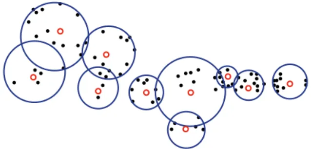
The RBC is a very simple randomized data structure that can be visualized as a horizontal slice of a metric tree with overlapping nodes. The data structure consists of nr
rep-resentative points R ⊂ X which are chosen uniformly at random, each of which points to a subset of the remainder ofX. In particular, for eachr∈R, the data structure main-tains a listLr which contains thes-nearest neighbors ofr
amongX. These lists can and should overlap. See figure 1 for an example.
Searching the RBC for a query q’s nearest neighbor is quite simple. First, the search algorithm computes the near-est neighbor ofqwithin the representative setRusing brute force search; suppose it is r∗. Next, the algorithm com-putes the NN ofqwithin the points owned byr∗—i.e. the
Figure 1: An example RBC. The black circles are database points, the red (open) circles are the repre-sentatives, and the blue balls cover the points falling into the nearest-neighbor list Lr for each represen-tative.
points contained within the listLr∗—again using brute force
search. The nearest neighbor withinLr∗ is returned.
This algorithm builds off of the intuition that two nearby points are likely to have the same representative, which can be justified with the triangle inequality. It is possible that the algorithm will return an incorrect answer, but the prob-ability of this event can be reduced by increasing the sizes of lists each representative points to and thereby increasing the overlap between lists, or by increasing the number of representatives.
Let us consider the work complexity of search. Brute force search for m queries among n elements in Rd takes work
O(mnd); moreover this operation parallelizes nearly linearly assuming m·n is larger than the number of processors.3 Thus if there are nr representatives, each of which ownss
database elements, the work required for search using a RBC is O(mnrd+msd), and this work is simple to distribute.
Clearly, the choice ofnrandsdictates the time complexity.
The choice of these two parameters also affects the prob-ability of success. The product of these two values nr ·s
should be greater than the size of the database n; if it is much smaller, there will be many database points which are not covered at all. On the other hand, since the algorithm only searches for NN among points within a single represen-tative’s list, increasing the overlap between lists will boost the probability of success. This idea is similar in spirit to the kd-trees with overlapping cells of [14].
The asymptotic time complexity is a function of the greater ofnr ands; hence from the perspective of time complexity,
we may as well set them equal. To ensure a reasonably low probability of failure, nr·sshould be greater thann. The
following choices satisfy these criteria:
nr=s=O(
√
nlogn). (1)
These choices ofnrandsyield a per-query work amount of
only O(d√nlogn), which is a dramatic improvement over theO(dn) work required of the brute force algorithm. This is a massive speedup for even moderate values ofn. 3On a GPU, one typically needs to create many more (soft-ware) threads than the number of thread processors so that the scheduler can hide certain latencies. Even so, the num-ber of threads needed to keep the processor busy is typically a very small fraction of the work to be done for NN prob-lems.
Intuitively, the logarithmic terms provide the necessary overlap between lists so that the probability of failure is small. Furthermore, as long as√nlogn is larger than the number of processors, the algorithm will still make full use of the GPU (but see the previous comment). We show in the experiments that a simple setting of the parameters yields both a significant speedup and a very low error rate.
One might view the RBC as a tree-based space decom-position data structure that has only one level. The space decomposition trees used on CPUs typically have a depth of logn, and so it is rather surprising that such a stump can be effective for the NN task. One could of course con-sider a tree of depth somewhere in between 1 and logn, and that might yield stronger results. On the other hand, as the depth is increased, the search algorithm becomes more and more difficult to parallelize and implement efficiently on a GPU. Regardless, we show in the experiments that this very simple structure offers more than a magnitude speedup over the (already very fast) standard brute force search algorithm on fairly challenging data sets.
5.
CONSTRUCTION OF THE RBC
The algorithm for constructing an RBC is simple to state: assign each database pointx∈Xto ther∈Rsuch thatxis one of thek-nearest neighbors ofr. Making this algorithm practical on a GPU requires some care, especially on large-scale data sets. We show in this section that the construction can be performed using a few naturally parallel operations. For each r ∈ R, we wish to construct a list Lr of the
id numbers ofr’s s-nearest neighbors. A straight-forward method for doing this is to use the brute force technique to do NN search betweenR and X, which we now detail. First, we compute all pairs of distances betweenX andR; if the resulting distance matrix is too big to fit in device memory, we process only a portion ofR at a time.4 The distances are stored in matrix D, where the rows index R
and the columns indexX. Next, we perform a partial sort (or selection) of each row of the distance matrix to find the
s-smallest elements. Doing so requires maintaining an index matrixJ of the same size asD. At the end of the sorting, the firsts elements of rowi of J are stored in Lri in the
device memory.
Unfortunately, the approach just detailed is not partic-ularly efficient. The problem is that the standard pivot-based selection and sort algorithms that are quite effective on the CPU are rather poorly suited for a GPU, requir-ing many irregular memory accesses. Thus one might re-sort to a partial selection re-sort algorithm as done in [7]. For very smalls, selection sort is quite effective (and simple to implement effectively on a GPU), however in our problem
s=O(√nlogn) and hence is too large for a work-inefficient sorting algorithm. For example, in the experiments we detail later,s is in the thousands. We found that the cost of the sorts dominated the cost of computing the distances even at much smaller values ofs. These findings are not surprising, given that sorting on GPUs is still very much an area of active research, and that even the best GPU algorithms are not dramatically faster than their CPU counterparts [19]. In contrast, the distance computation step is dramatically faster on the GPU as it is a basic matrix-matrix operation.
4If the databaseX does not fit into device memory, then it must be processed in smaller portions at a time.
To avoid these inefficiencies, we develop an alternative build algorithm. First we need a couple of definitions that are standard in the NN search literature. Therange search
problem is the sibling of NN search; instead of returning the closest point to a query, all points within a specified distance from the query are returned. The range count problem is the same as range search, but only the count of the number of points in range is returned. Both of these problems can clearly be solved with brute force search: compute all dis-tances and return points—or the count of points—in range. Our alternative build algorithm, like the simple one al-ready described, first computes the matrix of distances be-tween R and X. Instead of sorting the rows (recall there is one row per representative), it then performs a series of range counts to find a range γ such that approximately s
points fall within distance γ of r for eachr ∈ R. It then performs aγ-range search in which the ids of the (approxi-mately)sclosest points are returned.
We now go into the details of this algorithm. Each row of the distance matrix can be examined independently of the other rows, providing a natural granularity to parallelize at. Furthermore, each row is assigned a group oftthreads (t= 16 in the current implementation), which examine dif-ferent portions of the row. First, the algorithm finds the minimum and maximum values in each row. This is done in the obvious way; namely, each thread scans 1/16th of the row to find the min and max in that portion, then each thread writes its min and max to shared memory, and then the values are compared and written using the standard par-allel reduction paradigm.
With the mins and maxes calculated, the algorithm now has a starting guess for a range γi (where i refers to the
row) such that the number of points falling within distance
γi of reference pointriis s. The algorithm starts with the
average of the min and the max inγi, and performs a range
count. The division of labor into threads is the same as be-fore: there aretthreads assigned per row, and the rows can be processed independently.5 Once the count is computed, the rangesγiare adjusted, and another range count is
exe-cuted. This process repeats until the range counts are close enough tos, at which point the counts are stored into the main memory of the GPU. Note that since multiple rows are grouped onto the same multiprocessor, this procedure appears to be performing a data-dependent recursion, which is inefficient in the SIMD architecture of GPUs. However, the only place of divergence between threads (in different rows) is in choosing whether to increment or decrementγi,
as long as there is agreement on how many iterations to run for. Thus this algorithm makes only minor divergences be-tween threads and hence is effective within the constraints of the SIMD architecture.
The algorithm next takes theγis from the previous step
and performs a range search on this value of γi. For each
element of the distance matrix, the algorithm compares the distance to the appropriateγiand sets a binary variable (in
the main GPU memory) as appropriate. This step is trivial to parallelize.
Finally, the algorithm takes the binary matrix computed in the previous step and uses it to compute the ids of the database points to be stored in each Li. It does this by
performing a parallel compaction on the lists Li using the
5However, we found it more efficient to group several rows together into a common CUDA thread block.
Data DB Size Dimension # queries nr
Bio 200k 74 50k 1456 Physics 100k 78 50k 1024 Robot 1M 21 1M 3248
Table 2: Data specifications.
parallel prefix sum paradigm, which has been detailed specif-ically for GPUs in [20].
Though this build routine is a bit complicated, we found that it was significantly more efficient than the simple sort-based algorithm discussed at the beginning of this section. We attribute this efficiency to the minimal and regular in-teraction with main memory: each step of the range count reads the distance matrix once, as do the rest of stages of the algorithm, and the reads are simple to coalesce. Fur-thermore, there are few memory writes: theγi are written
in one step, the binary matrix in the next, and finally the lists Li. These writes follow a very regular pattern, and
so are also simple to coalesce. In contrast, a work-efficient sorting algorithm would likely need to perform many more writes.
We note that each step of the build algorithm parallelizes and can executed efficiently on graphics hardware. The total amount of work done is reasonably small. Comput-ing the distance matrix requires O(n·nrd) work, where
nr =O(
√
nlogn) is the number of representatives; and lo-cating the correct range requiresO(n·nrlog ∆) work. Here
∆ is thespread of the metric space, defined as the ratio of the maximum distance between points in the database to the minimum distance between points in the database.
6.
EXPERIMENTS
In this section, we measure the performance of the RBC data structure on several data sets. Our implementation is in CUDA and C, and is available from the author’s web-site. All experiments were conducted on a NVIDIA C2050 with three gigabytes of memory, running on a 2.4Ghz Intel Xeon.6 All of the real-valued variables were stored in single precision format, which is appropriate for the data we are experimenting with.
We used three data sets for experimentation; see table 2 for the basic specifications. The Bio and Physics data sets are taken from the KDD-Cup 2004 competition; see [10] for more details. These data sets have been experimented with extensively in the machine learning literature, and have been previously benchmarked for nearest neighbor search in [2, 4, 18]. The Robot data set is an inverse dynamics data set generated from a Barrett WAM robotic arm with seven degrees of freedom; see [15] for more information. We used the `1-norm to measure distance. We note that the data we use is all of moderately high dimensionality and hence is challenging for space-decomposition techniques.
It is non-trivial to implement algorithms on the GPU in an efficient way; slight changes in code can often lead to mas-sive differences in performance. Because of this sensitivity to implementation details, benchmarking analgorithm—as opposed to an implementation—is tricky. Here we measure the performance of our search algorithm relative to brute 6We also experimented with a NVIDIA GTX285 and found similar speedups.
Data Brute (sec) RBC (sec) Speedup Avg rank Bio 9.97 .20 49 .74 Physics 4.99 .14 35 1.34
Robot 408.23 3.35 122 .71
Table 3: Comparison of search time for RBC and brute force. The times stated are the times needed compute the nearest neighbors forall of the queries (e.g. 100k for the Bio data set).
force search on the GPU. At the core of the RBC search algorithm is a brute force search, albeit on subsets of the database, not the whole thing. To normalize for implemen-tation issues, we use virtually identical brute force imple-mentations for the RBC search and for the (full) brute force search.7 Additionally, as a sanity check, we compared the performance of our brute force implementation to one that was previously published by Garcia et al. in [7]. We found our implementation to be slightly faster than Garcia’s man-ual and CUBLAS-based implementations. We concluded that our implementation is reasonable for benchmarking the RBC search algorithm.
Since our algorithm is not guaranteed to return the exact nearest neighbor, we need to measure the error. To do so we compute the rank of the returned point—i.e. how many points in the database are closer to the query than the re-turned point. A rank of 0 corresponds to the (exact) first nearest neighbor, a rank of 1 to the second nearest neighbor, and so on. Note that in all three data sets there are 100k points, so a rank of 1 is a point among the closest.002% of points, a rank of 2 among the closest.003%,etc.
Our data structure has one parameter: nr, the number
of representatives (recall thatsis set equal tonr). Though
we suggested a setting of nr in section 4, in practice nr
will be set according to the time (or error) requirements of the system. Here we make a simple choice of nr = 1024
for a database of size n = 100k, and scale it up to the larger databases according to equation 1. This choice is an educated guess that seems to work well, but is essentially unoptimized. Refer back to table 2 for the exact numbers for each data set.
Perhaps the most common setting for NN search is the of-fline case: the data structure is built ofof-fline, and the quantity of interest is the retrieval time. We compare the time for search using brute force and for using RBC-based search. The results are shown in table 3.
In some situations, it does not make sense to separate the build time from the query time. We demonstrate that our build algorithm is quite efficient: even when the build time is taken into account, our method still affords roughly an order of magnitude speedup over brute force search. See table 4 for the numbers.
These results are quite strong. In particular, the RBC search algorithm yields a speedup over GPU-based brute force of one to two orders of magnitude with a very small amount of error. For the Bio and Physics data sets, this speedup is roughly comparable to the speedup of the
mod-7
The version used for the RBC search is slightly more in-volved, as it needs to access a stored mapping from thread indices to database elements.
Data Total time (sec) Bio 1.28 Physics .65
Robot 11.92
Table 4: Total computation time (i.e. the build and search time) for the RBC experiments.
ern metric tree variants over brute force on a CPU.8 As we remarked earlier, the GPU-based brute force procedure is already competitive with these tree approaches for this data. For the Robot data set, we are getting an average query time of less than 4µs, even though the database con-tains one million points. Note also that the performance relative to brute force is improving as the problem size gets larger. This is not surprising, given that the complexity of search isO(√nlogn), but it is a useful property of the al-gorithm. Finally, we again emphasize that the data is fairly high-dimensional and so is challenging for any space decom-position scheme—on the GPU or CPU.
7.
CONCLUSIONS
We introduced an exceedingly simple data structure for nearest neighbor search on the GPU, with search and build algorithms that are efficient on parallel systems. Our ex-periments are quite promising: despite the difficulties as-sociated with working on GPUs, our algorithm is able to outperform GPU-based brute force search convincingly on several challenging data sets. There is a tremendous amount of future work to be done, including a theoretical analysis of the search algorithm and a more careful investigation of the effect of the algorithm parameters on performance. Fur-thermore, there is still considerable room for improvement in our implementation.
8.
ACKNOWLEDGMENTS
I thank my colleagues in the Empirical Inference Depart-ment for helpful discussions and encourageDepart-ment. Thanks to Duy Nguyen-Tuong for providing the robot data.
9.
REFERENCES
[1] S. Arya, D. M. Mount, N. S. Netanyahu,
R. Silverman, and A. Wu. An optimal algorithm for approximate nearest neighbor searching.Journal of the ACM, 45(6):891–923, 1998.
[2] A. Beygelzimer, S. Kakade, and J. Langford. Cover trees for nearest neighbor. InProceedings of the International Conference on Machine Learning, 2006. [3] S. Brin. Near neighbor search in large metric spaces.
InProceedings of the 21th International Conference on Very Large Data Bases, 1995.
[4] L. Cayton and S. Dasgupta. A learning framework for nearest neighbor search. InAdvances in Neural Information Processing Systems 20, 2007.
[5] K. L. Clarkson. Nearest-neighbor searching and metric space dimensions. InNearest-Neighbor Methods for Learning and Vision: Theory and Practice, pages 15–59. MIT Press, 2006.
8
The Robot dataset has not been previously benchmarked.
[6] T. Foley and J. Sugerman. KD-tree acceleration structures for a GPU raytracer. InProceedings of Graphics Hardware, 2005.
[7] V. Garcia, E. Debreuve, and M. Barlaud. Fast k nearest neighbor search using GPU. In CVPR Workshop on Computer Vision on GPU (CVGPU), 2008.
[8] P. Indyk and R. Motwani. Approximate nearest neighbors: towards removing the curse of
dimensionality. InProceedings of the 30th annual ACM Symposium on Theory of Computing (STOC), 1998. [9] D. R. Karger and M. Ruhl. Finding nearest neighbors
in growth-restricted metrics. InProceedings of the 34th Annual Symposium on Theory of Computing (STOC), 2002.
[10] KDD cup competition, 2004.
http://kodiak.cs.cornell.edu/kddcup.
[11] R. Krauthgamer and J. R. Lee. Navigating nets: simple algorithms for proximity search. InProceedings of the 15th Annual Symposium on Discrete Algorithms (SODA), 2004.
[12] C. Lauterbach, M. Garland, S. Sengupta, D. Luebke, and D. Manocha. Fast BVH construction on GPUs. In
Proc. Eurographics, 2009.
[13] C. Lauterbach, Q. Mo, and D. Manocha. gProximity: Hierarchical GPU-based operations for collision and distance queries. InProc. Eurographics, 2010. [14] T. Liu, A. W. Moore, A. Gray, and K. Yang. An
investigation of practical approximate neighbor algorithms. InAdvances in Neural Information Processing Systems, 2004.
[15] D. Nguyen-Tuong and J. Peters. Using model knowledge for learning inverse dynamics. InProc. IEEE International Conference on Robotics and Automation, 2010.
[16] S. Omohundro. Five balltree construction algorithms. Technical report, ICSI, 1989.
[17] D. Patterson. The trouble with multicore.IEEE Spectrum, July 2010.
[18] P. Ram, D. Lee, H. Ouyang, and A. Gray.
Rank-approximate nearest neighbor search: Retaining meaning and speed in high dimensions. InAdvances in Neural Information Processing Systems 22, 2009. [19] N. Satish, M. Harris, and M. Garland. Designing efficient sorting algorithms for manycore GPUs. In
Proc. IEEE International Parallel and Distributed Processing Symposium, 2009.
[20] S. Sengupta, M. Harris, Y. Zhang, and J. D. Owens. Scan primitives for GPU computing. InProceedings of Graphics Hardware, 2007.
[21] J. K. Uhlmann. Satisfying general
proximity/similarity queries with metric trees.
Information Processing Letters, 40:175–179, 1991. [22] V. Volkov and J. W. Demmel. Benchmarking GPUs to
tune dense linear algebra. InProceedings of the 2008 ACM/IEEE conference on Supercomputing, 2008. [23] K. Zhou, Q. Hou, R. Wang, and B. Guo. Real-time
kd-tree construction on graphics hardware.ACM Trans. Graph., 27(5):126, 2008.