ELUCIDATING ENERGY AND ELECTRON TRANSFER DYNAMICS WITHIN MOLECULAR ASSEMBLIES FOR SOLAR ENERGY CONVERSION
Zachary Aaron Morseth
A dissertation submitted to the faculty of the University of North Carolina at Chapel Hill in partial fulfillment of the requirements for the degree of Doctor of Philosophy in the Department
of Chemistry
Chapel Hill 2016
ii © 2016
iii ABSTRACT
Zachary Aaron Morseth: Elucidating Energy and Electron Transfer Dynamics within Molecular Assemblies for Solar Energy Conversion
(Under the direction of John M. Papanikolas)
The use of sunlight to make chemical fuels (i.e. solar fuels) is an attractive approach in the quest to develop sustainable energy sources. Using nature as a guide, assemblies for artificial photosynthesis will need to perform multiple functions. They will need to be able to harvest light across a broad region of the solar spectrum, transport excited-state energy to charge-separation sites, and then transport and store redox equivalents for use in the catalytic reactions that produce chemical fuels. This multifunctional behavior will require the assimilation of multiple
components into a single macromolecular system. A wide variety of different architectures including porphyrin arrays, peptides, dendrimers, and polymers have been explored, with each design posing unique challenges. Polymer assemblies are attractive due to their relative ease of production and facile synthetic modification. However, their disordered nature gives rise to stochastic dynamics not present in more ordered assemblies. The rational design of assemblies requires a detailed understanding of the energy and electron transfer events that follow light absorption, which can occur on timescales ranging from femtoseconds to hundreds of
iv
view of these dynamics. This thesis provides an overview of work on single-site molecular assemblies and polymers decorated with pendant chromophores, both in solution and on
v
vi
ACKNOWLEDGEMENTS
First, I would like to thank my family, especially my parents Aaron and Angela Morseth, for their guidance and support throughout my life. Their value of my education and teaching me a strong work ethic has undoubtedly led me to where I am today. Second, I thank my loving wife, Tory Morseth, for her support and pushing me to be the best person I can possibly be. While graduate school has had its fair share of ups and downs, she stood by my side each and every day with a strong will to see me succeed professionally and personally.
I also would like to thank my teachers and mentors through all walks of my life. Most importantly, I thank Lowell Nelson for instilling a passion for science in me and appreciation of the scientific method. I must also thank the faculty at Minnesota State University – Moorhead for taking that passion and molding me into the scientist that I am today. I especially thank Asoka Marasinghe, Craig Jasperse, Jeffrey Bodwin, Adam Goyt, and Justin James for their mentoring and friendship during my undergraduate education.
vii
TABLE OF CONTENTS
LIST OF TABLES.………...xiv
LIST OF SCHEMES.………....xv
LIST OF FIGURES.……….xvi
LIST OF ABBREVIATIONS……….xxxi
LIST OF SYMBOLS ………...xxxiii
CHAPTER 1. INTRODUCTION ……….………..1
1.1. INTRODUCTION……… ..1
1.2. ARTIFICIAL PHOTOSYNTHESIS……….…..2
1.3. PHOTOINDUCED DYNAMICS IN MOLECULAR ASSEMBLIES………….…..4
1.3.1. Polymer Structures………...5
1.3.2. Site-to-Site Energy Transport………..7
1.3.3. Dynamics in Polymer Assemblies with π-Conjugated Polymer Backbone.………....12
1.3.4. Multifunctional Behavior………...19
viii
CHAPTER 2. ROLE OF MACROMOLECULAR STRUCTURE IN THE ULTRAFAST ENERGY AND ELECTRON TRANSFER DYNAMICS
OF A LIGHT-HARVESTING POLYMER………...25
2.1. INTRODUCTION………..25
2.2. EXPERIMENTAL METHODS………...…..29
2.2.1. Sample Preparation……….……….29
2.2.2. Steady State Techniques………..29
2.2.3. Time-Resolved Emission Spectroscopy……….….29
2.2.4. Transient Absorption Spectroscopy……….30
2.2.5. Electronic Structure Calculations………31
2.3. RESULTS AND DISCUSSION……….33
2.3.1. Synthesis of pF-iI polymer Assembly……….….33
2.3.2. Static Spectroscopy……….……….33
2.3.3. Ultrafast Spectroscopy……….34
2.3.3.1. Isoindigo Excited-State Dynamics………34
2.3.3.2. Energy and Electron Transfer Quenching of the Polymer Excited State………..……….…………37
2.3.3.3. Spectral Modeling of the pF-iI Spectra……….41
2.3.4. Simulation of Excited State Quenching Dynamics………..45
2.3.4.1. Macromolecular Polymer Structures……….45
2.3.4.2. Kinetic Network………49
ix
2.3.4.4. Electron Transfer………..53
2.3.4.5. Time-Dependent Populations………54
2.3.4.6. Comparison of Simulation with Experimental Observation…….55
2.3.5. Analysis of Simulation Results………57
2.3.5.1. Microscopic Picture……….….57
2.3.5.2. Ensemble Quenching Dynamics………...61
2.3.5.3. Role of Macromolecular Structure………62
2.4. CONCLUSIONS………..……….……..67
2.5. REFERENCES………...68
CHAPTER 3. ELECTRON TRANSFER DYNAMICS IN AN ISOINDIGO LOADED POLY(THIOPHENE) ASSEMBLY………71
3.1. INTRODUCTION………..71
3.2. EXPERIMENTAL METHODS………..75
3.2.1. Sample Preparation………...75
3.2.2. Steady State Techniques………...75
3.2.3. Transient Absorption Spectroscopy………...…..75
3.2.4. Electronic Structure Calculations………77
3.2.5. Electrochemical Measurements……….………...77
x
3.3. RESULTS AND DISCUSSION……….……….…...79
3.3.1. Synthesis of Materials………..79
3.3.2. Static Spectroscopy………..79
3.3.3. Ultrafast Spectroscopy………..………...83
3.3.3.1. Isoindigo Excited-State Dynamics……….………...83
3.3.3.2. Ultrafast Quenching of the Polymer Excited State…….………..85
3.3.3.3. Charge Recombination………..………91
3.3.4. Simulation of Excited State Quenching……….………..92
3.3.4.1. Development of the Kinetic Model…………...………94
3.3.4.2. Comparison with Experiment………...99
3.3.4.3. Microscopic Analysis of Simulation Results………….……….101
3.3.4.4. Ensemble ET Quenching Dynamics ………..103
3.4. CONCLUSIONS………..…107
3.5. REFERENCES………...108
CHAPTER 4. POLYMER-BASED RUTHENIUM(II) POLYPYRIDYL CHROMOPHORES FOR SOLAR ENERGY CONVERSION APPLICATIONS.………....111
4.1. INTRODUCTION………111
4.2. EXPERIMENTAL METHODS………115
xi
4.2.2. Steady State Techniques………..……..115
4.2.3. Time-Resolved Emission Spectroscopy………...…….115
4.2.4. Transient Absorption Spectroscopy………..…….116
4.2.5. Transient Absorption Kinetics Fitting Parameters……….117
4.2.6. Electronic Structure Calculations………..……117
4.2.7. Molecular Dynamics Simulations……….……….117
4.3. RESULTS AND DISCUSSION……….………..119
4.3.1. Static Spectroscopy………119
4.3.2. Macromolecular Polymer Structures………...………..119
4.3.3. Time-Resolved Spectroscopy………122
4.4. CONCLUSIONS………..130
4.5. REFERENCES……….……131
CHAPTER 5. LIGHT-HARVESTING AND CHARGE SEPARATION IN A -CONJUGATED ANTENNA POLYMER BOUND TO TiO2…………..……..…….134
5.1. INTRODUCTION………..…..134
5.2. EXPERIMENTAL METHODS………...137
5.2.1. Sample Preparation………...….137
5.2.2. Steady State Techniques………....137
5.2.3. Transient Absorption Spectroscopy………...137
xii
5.2.5. Molecular Dynamics Simulations……….…….139
5.3. RESULTS AND DISCUSSION………..….141
5.3.1. Polymer Structures……….…141
5.3.2. Photoexcitation of pF-Ru-A………..……….142
5.3.3. Interfacial Dynamics of pF-Ru-A………..………143
5.4. CONCLUSIONS……….…….151
5.5. REFERENCES……….152
CHAPTER 6. INTERFACIAL DYNAMICS WITHIN AN ORGANIC CHROMOPHORE-BASED WATER OXIDATION MOLECULAR ASSEMBLY………..155
6.1. INTRODUCTION………155
6.2. EXPERIMENTAL METHODS……….………...158
6.2.1. Sample Preparation……….………….…..158
6.2.2. Steady State Techniques……….….…………..158
6.2.3. Transient Absorption Spectroscopy………..………….159
6.2.4. Electronic Structure Calculations………..161
6.3. RESULTS AND DISCUSSION……….………..162
6.3.1. Photoexcitation and Electronic Structure of T3-trpy and T3-trpy-Ru-L……….162
6.3.2. Photophysics of T3-trpy Chromophore………..…………165
xiii
6.3.2.2. Interfacial Dynamics on TiO2……….…167
6.3.3.3. Interfacial Dynamics on SnO2………169
6.3.3. Photophysics of T3-trpy-Ru-L Assembly………...……171
6.3.3.1. Solution Dynamics……….….171
6.3.3.2. Interfacial Dynamics on TiO2………...…..174
6.3.3.3. Interfacial Dynamics on SnO2………..……..177
6.4. CONCLUSIONS………...…….179
xiv
LIST OF TABLES
Table 1.1. Energy and electron transfer data for π-conjugated polymer assemblies
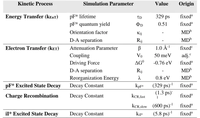
with pendant RuII chromophores……….17 Table 2.1. Simulation parameters used in the kinetic modeling of pF-iI……….……….51 Table 3.1. Simulation parameters used in the kinetic modeling for photoinduced
dynamics of the pT-iI assembly……….……..98 Table 4.1. TRES decay fits for TiO2//pS-Ru-A and ZrO2//pS-Ru-A films monitored
xv
LIST OF SCHEMES
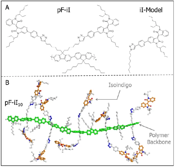
Scheme 2.1. (Top) Depiction of the pF-iI10 polymer assembly with the indices
of the fluorene monomers (Fi) and the iI pendants (iIj). (Bottom) Illustration
of the kinetic network used to describe the photoinduced dynamics in the pF-iI polymer assemblies following excitation centered on a fluorene
monomer………...50 Scheme 3.1. Illustration of the fundamental photophysical events occurring within
the pT-iI assembly……….………....97 Scheme 4.1. Cartoon of pS-Ru-A (obtained from molecular dynamics simulations)
anchored onto a TiO2 surface, displaying the primary photophysical
events………...………...112 Scheme 4.2. Schematic representation of the photophysical events of the pS-Ru-A
assembly at the surface of TiO2. The blue circles represent Ru(L)32+
chromophores while the green and red circles correspond to Ru(L)33+
and Ru(L)32+*……….……….114
Scheme 5.1. Cartoon of pF-Ru-A anchored onto a TiO2 surface………....136 Scheme 5.2. Schematic representation of photophysical events of pF-Ru-A on
the surface of TiO2. Balls represent Ru(L)32+ chromophores, and the
grey ribbon the poly(fluorene) backbone………144 Scheme 6.1. (Left) Energy level diagram of the relevant states present in the T3-trpy
chromophore and T3-trpy-Ru-L assemblies in relation to the metal oxide
conduction band density of states for TiO2 (top) and SnO2 (bottom).
(Right) Illustration of the interfacial dynamics within the T3-trpy-Ru-MeCN (top) and T3-trpy-Ru-OH2 (bottom)
xvi
LIST OF FIGURES
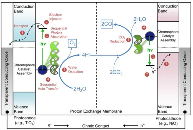
Figure 1.1. Schematic diagram of a tandem DSPEC for solar-driven splitting of
CO2 into CO and O2………..……….………...3
Figure 1.2. Condensed phasepolymer assembly structures obtained from molecular dynamics simulations. Structures were calculated using periodic
boundary conditions in the presence of explicit acetonitrile solvent and PF6- counter ions. The polymer scaffold is shown in green color
and the Ru atoms are depicted as orange spheres with enlarged diameters. A portion of the solvent is shown in the
pF-Ru16 structure………..….…….6
Figure 1.3. (Left) Time resolved emission monitoring OsII photoluminescence
in pS-Ru17Os3 and pF-Ru60Os10. (Right) Illustration of site-to-site
energy transport within a subsection of pS-Ru17Os3 (upper) and
pF-Ru60Os10 (lower). The initial Ru excited state (blue) undergoes
energy transfer to adjacent Ru complexes and is ultimately
transferred to the Os trap (red)… ………11 Figure 1.4. Condensed phase structure of a 40-repeat unit pF in explicit
acetonitrile solvent obtained from molecular dynamics simulations. Most of the solvent is omitted for clarity, but a portion is shown for scale. The conformational subunits are colored based on the energy level with darker shades indicating subunits with shorter lengths and hence higher energies. The enlarged section shows a zoomed-in view of adjacent conformational
subunits with a conjugation break……….……….. 13
Figure 1.5. (Left) Illustration of excitonic energy transfer (top) and excited-state self-trapping by torsional relaxation (bottom) along a π-conjugated polymer backbone following excitation into a high-energy conformational subunit. (Right) Transient absorption difference spectra of unfunctionalized pF (upper)
and pT (lower) from 300 fs to 1.4 ns following 388 nm excitation……… 14 Figure 1.6. Transient absorption spectra following primary excitation of the polymer
backbone at 388 nm for pF-Ru (upper left) and pT-Ru (upper right). (Bottom) RuII absorbance (εA(λ)) and normalized (to unit area) polymer emission spectra (FD(λ)). The shaded grey area reflects the integrand, FD(𝜆)𝜖𝐴(𝜆)𝜆4, which is scaled for clarity. (Right) Kinetic traces
of the polymer assemblies showing the initial polymer excited-state
quenching during the first 10ps following excitation………..….16 Figure 2.1. (A) Chemical structures of the pF-iI repeat unit and iI-Model.
xvii
The solvent is excluded for clarity……….……….………..28 Figure 2.2. Ground state absorbance spectra of the pF-iI assembly (dark grey),
pF (blue), and iI-Model (red) in room temperature DCM solution Also shown is the superposition of the iI-Model and pF
absorbance spectra (dashed black)………..………. 34 Figure 2.3. (Left) Absorbance spectrum of iI-Model complex in DCM (red) and
theoretical transitions predicted from TD-DFT calculations (gray bars). The primary orbitals corresponding to each transition are also shown for the dominant visible transitions. (Right) Calculated isodensity plots of the frontier molecular orbitals (LUMO+1,LUMO, HOMO, HOMO-1, HOMO-2, and HOMO-3) of the iI-Model complex (isodensity value =
0.03)………. ………..…...35 Figure 2.4. Femtosecond transient absorption spectra following photoexcitation
at 595 nm (150 fs, 280 nJ with a 120 µm spot size) in DCM at
0.3, 1, 2, 5, 15, and 20 ps for iI-Model (A) and pF-iI (B). Also shown in (A) is the inverted ground-state absorbance spectrum of iI-Model in DCM, normalized to the 410 nm GSB (shaded orange)
(C) Decays of the transient signals at 640 nm for iI-Model (orange circles) and pF-iI (red triangles). Both transients exhibit single exponential
decays with τ = 5.8 ± 0.1 ps. All spectra were measured in argon
saturated DCM solution at room temperature………...36 Figure 2.5. (A) Transient absorption spectra of pF in DCM at 0.2, 1, 15, 50,
150, 500, and 1000 ps. Excitation was at 388 nm and the pulse energy was 10 nJ/pulse. (B) Transient absorption spectra of pF-iI in DCM at 0.15, 0.3, 0.5, 1, 1.5, and 3 ps. Excitation was at 388 nm and the pulse energy was 60 nJ/pulse. (C) Transient absorption spectra of pF-iI in DCM at 1.5, 3, 5, 25, 50, 300, and 1000 ps. (D) Evolution of the pF SE bands, as indicated in (A).
(E) Evolution of the SE bands in pF-iI, as indicated in (B).
(F) Comparison of the decays of the transient signals at 440 nm for pF-iI (red circles) and pF (black circles) show significant quenching of pF* in pF-iI within 10 ps of excitation. Both exhibit bi-exponential decays: pF-iI (τ1= 0.52 ± 0.1 ps and τ2 = 1.4 ± 0.2 ps) and pF
(τ1= 25 ± 5 ps and τ2 = 325 ± 15 ps)……… ………..38 Figure 2.6. (Left) Time-resolved fluorescence spectra of the unfunctionalized
pF homopolymer in argon saturated DCM following 388 nm excitation. (Right) Singlet lifetime of the unfunctionalized pF homopolymer following 388 nm excitation. The fsTA transient at 780 nm (black circles) and tri-exponential fit (red line) are shown along with the scaled time-resolved fluorescence decay
xviii
Figure 2.7. (Left) Spectroelectrochemical difference spectrum of iI (black) and pF (red) following quantitative reduction and oxidation, respectively. The pF+ spectrum has been scaled by a factor of 4.5 to account for the polaron length resulting from oxidation of the pF backbone.
(Right) Predicted spectrum for the CS state obtained by adding the pF+ and iI- difference spectra (grey dashed line) scaled to match the 1000 ps spectra following excitation of pF-iI at 388 nm (dark red line). Shown in the inset is a zoomed in view of the pF+ absorption, as
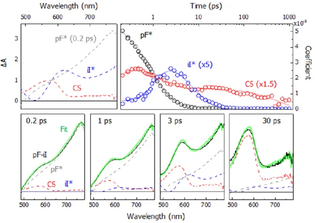
indicated by the black dashed line………...….40 Figure 2.8. (Top, left) Spectral contributions from pF* (0.2 ps), iI*, and the
CS state used in the spectral modeling, normalized at 580 nm.
(Top, right) Time-resolved coefficients for pF* (black), iI* (blue), and the CS state (red) spectral contributions obtained from least-squares analysis of the modeled pF-iI transient absorption spectrum. The iI* and CS populations have been scaled for clarity. Overlaid on the pF* and iI* populations are bi-exponential fits while a tri-exponential fit is overlaid on the CS state population. (Bottom, left to right) Modeled pF-iI spectra at 0.2, 1, 3, and 30 ps with the modeled spectrum (green) overlaid on the pF-iI assembly spectrum (black). The individual spectral contributions for pF* (gray), iI* (blue), and the CS state (red) are shown as dashed
lines………..………...….44 Figure 2.9. Snapshot of the orthorhombic (100x55x55 Å) simulation cell
consisting of 10 fluorene monomers (green), 10 isoindigo pendants (orange), and 2,500 dichloromethane molecules used for molecular dynamics (MD) simulations of the pF-iI10 polymer assembly. The MD simulations were collected on relaxed polymer structures for 1 ns
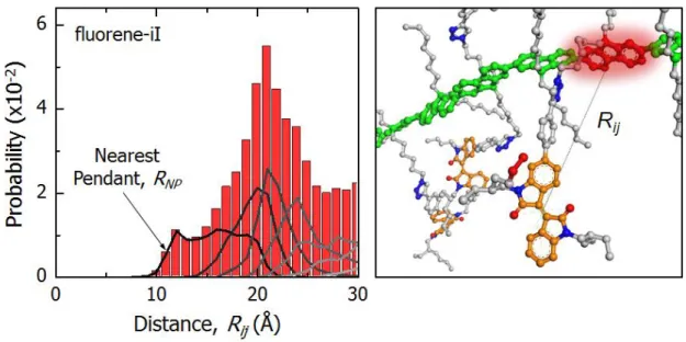
with periodic boundary conditions………..………….46 Figure 2.10. (Left) Distance distributions for fluorene-isoindigo from the ensemble
of pF-iI polymer structures obtained from the MD simulations. The bars represent the total distribution while the lines represent the successive nearest acceptors. (Right) Illustration of the fluorene-isoindigo through- space distance (Rij), where the distance is computed between centroids
placed on each unit………..……….48 Figure 2.11. iI-Model absorbance (red) and pF emission spectrum (blue) normalized
to unity area showing the scaled Förster overlap integrand shaded in gray……….…..53 Figure 2.12. Comparison of the pF*, iI*, and CS state populations obtained from
experiment (black circles) with the simulated populations (red line). The spectral amplitudes for each species were scaled to match the
magnitude of the simulated populations……...………...………56 Figure 2.13. (Left) Model isoindigo and fluorene oligomer pair used for the
xix
computational package.6 The distance is computed from centroids
placed on each unit. (Right) Plot of log(coupling) versus distance obtained from calculation of the charge transfer integrals of the model systems for
pF-iI…...………...…57 Figure 2.14. (A, B) Pictorial representation of the kinetic model applied to
representative pF-iI10 polymer structures obtained from molecular dynamics simulations. The initial exciton is shown as a red cloud along the polymer backbones, in which the energy and electron transfer rates are computed from the distances and orientation factors. The total quenching rate of the ith monomer (kQ,i) is then expressed as the sum of the individual
computed rates. The magnitude of the EnT rate constant to the nearest pendant (i.e,
k
EnTNP ) is given as the cross-hatched rectangle for eachconfiguration………...………..60 Figure 2.15. Distribution of rate constants from the pF-iI kinetic simulations,
showing the total quenching rate distribution (black line). Also shown is the mean energy transfer efficiency computed as a function of the total quenching rate constant (kQ,i) from each configuration. The total rates
were computed for each configuration and binned on a logarithmic scale
ranging from 1010 to 1015 s-1 with a total of 500 bins………...…62 Figure 2.16. (A) Median energy transfer rate constants as a function of the
total energy transfer rate constant to the nearest pendant (purple line) and to the pendant with the largest rate (green line). (B) Mean number of acceptors (orange circles) that are needed to achieve 80% of the total energy transfer quenching rate in the kinetic simulations. (C) Mean donor-acceptor distance as a function of the total EnT quenching rate constant to the nearest pendant (purple) and to the pendant with the largest rate (green). (D) Mean orientation factor that gives rise to the computed EnT rates in pF-iI. The rates were computed for each configuration and binned on a logarithmic scale
ranging from 1010 to 1015 s-1 with a total of 500 bins……….……..64 Figure 2.17. Average fraction of the total energy transfer rate constant (kEnT,i)
computed as a function of kEnT,i for the pendant with the largest rate
(
k
EnTM ) and for the nearest pendant (k
EnTNP ) in each initial polymerconfiguration………...………..66 Figure 3.1. (Top) Chemical structures of the pT-iI monomer (left) and iI-Model
(right). (Bottom) Snapshot of a 15 repeat unit pT-iI polymer assembly (i.e., pT-iI15) obtained from fully atomistic molecular dynamics simulations in explicit dichloromethane (DCM) solvent. The polymer backbone is depicted in green and the iI pendants in orange. The
xx
Figure 3.2. Ground state absorbance spectra of the pT-iI polymer assembly (grey), unfunctionalized pT polymer (blue), iI-Model (red), and the
sum of the iI and pT absorbance spectra (dashed black). ………...81 Figure 3.3. Frontier orbitals (HOMO and LUMO) of geometry optimized
isoindigo dimers at varying separations obtained from density functional theory calculations using the B3LYP functional and the
6-31(d,p) basis sets, as implemented in Gaussian09 (Revision E.01)…… ……...82 Figure 3.4. (A) Femtosecond transient absorption difference spectra of
iI-Model in DCM at 0.3, 1, 2, 5, 15, and 20 ps. Shown shaded in orange is the inverted ground-state absorbance spectrum for iI-Model, normalized to the GSB at 410 nm. (B) Decay of the transient signal for iI-Model at 640 nm. The transient exhibits a single exponential decay with τ= 5.8 ± 0.2 ps. (C) Femtosecond transient absorption difference spectra of pT-iI in DCM at 0.3, 2, 5, 15, 30, and 100 ps. (D) Decay of the transient signal for pT-iI at 640 nm. The transient exhibits a single exponential decay with τ= 12.2 ± 1.0 ps. All spectra were measured in argon saturated DCM and excited with a 150 fs, 100 nJ pulse at
595 nm with a 120 μm spot size………..…...84 Figure 3.5. Franck-Condon mode analysis for the alkyl-substituted pT
emission spectra. The emission spectrum (red line) was fit to a sum of 4 Gaussian functions with constant width and mode
spacing (light purple line)………..86 Figure 3.6. (A) Transient absorption spectra of pT in DCM at 0.2, 3, 10, 100,
250, 500, 1000, and 1500 ps. Excitation was at 460 nm and the pulse energy was 15 nJ/pulse. (B) Transient absorption spectra of pT-iI in DCM at 0.25, 0.45, 1, 3, 7, 18, 25, 35, 95, 200, and 1500 ps. Excitation was at 460 nm and the pulse energy was 60 nJ/pulse. (C) Spectral modeling of the 1500 ps pT-iI spectrum (light red). The dashed red line, labeled CS State, is the sum of the iI- and pT+ spectra acquired from
spectroelectrochemical measurements (Figure 3.9). The dashed green line, labeled 3pT, is the 1500 ps pT spectrum from panel (A). The dark red line represents the sum of the CS State and 3pT spectra to produce the modeled 1500 ps spectrum. (D) Kinetics trace at 575 nm for pT-iI fit to a
bi-exponential function that exhibits a growth (τ1= 0.23 ± 0.08 ps) and
a decay (τ2 = 22.9 ± 0.6 ps)…………..………..….…..87 Figure 3.7. Decay of the pT* stimulated emission band at 620 nm versus time.
The transient was fit to a sum of two exponentials, with characteristic time
constants of τ1 = 1 ± 0.03 ps and τ2 = 490 ± 5 ps………...…88 Figure 3.8. (Left) Transient absorption spectra of pT in DCM from 1 ns to 10 μs
xxi
a single exponential decay with τ=13.7±0.8 μs………89 Figure 3.9. (Top) Spectroelectrochemical difference spectrum of pT+. (Middle)
Spectroelectrochemical difference spectrum of iI-Model. (Bottom) Modeled CS state obtained by adding the pT+ spectrum to 25% of the intensity of the iI- difference spectrum. The factor of 0.25has been introduced to properly account for the relative contributions of pT+
and iI- to the CS state spectrum. This stems from the fact that approximately 4 times as many reduced iI complexes can be accommodated by a single
positive polaron along an individual polymer chain.32………...……....90 Figure 3.10. Transient absorption decay for pT-iI following 460 nm excitation
monitoring the charge recombination kinetics at 800 nm. The signal was fit to a tri-exponential function, in which the fast time components (τ1 = 2.6 ps and τ2 = 21 ps) are attributed to the quenching dynamics and relaxation of iI*. The slower component (τ3 = 215 ps) is ascribed to
charge recombination between pT+ and iI-………...92 Figure 3.11. Snapshot of the orthorhombic simulation cell with dimensions of
85x50x50 Å consisting of 15 thiophene monomers (green), 15 isoindigo pendants (orange), and 1,800 dichloromethane molecules used for molecular dynamics (MD) simulations of the pT-iI15 polymer assembly. The MD simulations were collected on relaxed polymer structures for
1 ns with periodic boundary conditions………...………….…....93 Figure 3.12. (A) Total distance distributions for thiophene-isoindigo (T-iI)
and (B) isoindigo-isoindigo (iI-iI) from the ensemble of polymer structures obtained from MD simulations. The bars represent the total distribution while the shaded areas are the nearest isoindigo distance distributions from the perspective of each thiophene monomer (A)
and each isoindigo pendant (B)………...…..94 Figure 3.13. iI-Model absorbance (red) and pF emission spectrum (blue)
normalized to unity area showing the scaled Förster overlap integrand
shaded in gray………...95 Figure 3.14. Comparison between the pT-iI experimental kinetics at 575 nm
(black circles) and the linear combination of the simulated photoinduced
populations (red line) described by equation 3.4……….100 Figure 3.15. (Left) Model isoindigo and tetrathiophene oligomer pair used for the
estimation of the close-range electronic coupling (V0) with the ADF
computational package. The distance is computed from centroids placed on each unit. (Right) Plot of ln(Coupling) versus distance obtained from
calculation of the charge transfer integrals of the model system………….…..….101 Figure 3.16. Graphical illustration of the kinetic model applied to a representative
xxii
exciton is shown as a red cloud along the polymer backbone, in which the energy and electron transfer rates are computed using the distances and orientation factors. The total quenching rate is expressed as the sum of the
individual computed rates………..…….103 Figure 3.17. (Top) Distribution of total quenching rate constants from the pT-iI
kinetic simulations (black line). The gray shaded area reflects quenching rates that lie outside of the ultrafast transient absorption instrument response. The total rates were computed for each configuration and binned on a logarithmic scale ranging from 108 to 1015 s-1 with 500 bins. (Middle) Average electron transfer efficiency (red circles) computed as a function of the total quenching rate constant from each configuration. (Bottom) Average number of acceptors that are needed to achieve 80% of the total electron transfer quenching rate (black squares). The
standard deviation for each measurement is shown as the light gray bar…………..106 Figure 4.1. Ground state absorbance spectrum of the pS-Ru-A assembly on the
surface of TiO2 (blue line) and the emission spectrum of the pS-Ru-A assembly on ZrO2 following 480 nm excitation (red line). All films were immersed in acetonitrile with 100 mM LiClO4. Also shown is
the absorbance spectrum contribution from TiO2 (shaded gray area)…………....119 Figure 4.2. Optimized geometry of the pS-Ru monomer along with calculated
isodensity plots of the frontier molecular orbitals (LUMO+2,
LUMO+1, LUMO, HOMO) (isodensity value = 0.03) …….… ……….120 Figure 4.3. (Left) Ensemble radial distribution functions for distances computed
between Ru pendants from molecular dynamics simulations of pS-Ru-A in MeCN (top) and MeOH (bottom). (Right) Snapshot of a solvated pS-Ru-A chain in MeCN solvent, revealing the close-packed structure facilitated by the flexible pS backbone (green). Solvent molecules and
counter ions have been omitted for clarity………..………121 Figure 4.4. Radius of gyration computed from molecular dynamics simulations
of pS-Ru-A in MeCN (blue) and MeOH (red). The radii are centered at
16.9 and 20.9 Å for MeCN and MeOH, respectively……….122 Figure 4.5. Time-resolved emission for TiO2//pS-Ru-A and ZrO2//pS-Ru-A
monitored at 660 nm following 444 nm excitation. The decays are fit to a tri-exponential function, with time constants and amplitudes listed
in Table 4.1……….………....123 Figure 4.6. (A) Transient absorption spectra following 420 nm excitation of
xxiii
TiO2//Ru-A (green circles) and TiO2//pS-Ru-A (red circles) with the
bi-exponential fits overlain……….127 Figure 4.7. Kinetics traces at 480 nm on timescales ranging from 200 fs to
100 μs for ZrO2//Ru-A (black triangles), TiO2//Ru-A (blue triangles),
and TiO2//pS-Ru-A (red triangles)……….. ………… ……….….129 Figure 5.1. Chemical structures of Model-Ru-A, pF-Ru and pF-Ru-A………142 Figure 5.2. Ground-state absorbance spectrum of pF-Ru-A on TiO2 (blue)
and emission spectrum of pF-Ru-A on ZrO2 in MeCN with 0.1 M LiClO4.
The emission spectrum was acquired following excitation at 450 nm…………...143 Figure 5.3. (A)Transient absorption spectra following 450 nm laser excitation
for the Model-Ru-A complex on TiO2 at 0.25, 1, 5, 10, 100, and 1400 ps.
(B) Model-Ru-A//TiO2 kinetics trace at 385 nm. (C) Transient
absorption spectra of pF-Ru-A//TiO2 at 0.25, 1, 5, 10, 100, and
1400 ps. (D) pF-Ru-A//TiO2 kinetics trace at 385 nm. The films
were immersed in argon-saturated acetonitrile with 0.1 M LiClO4……….…146
Figure 5.4. Transient absorption spectra of pF-Ru-A//ZrO2 following photoexcitation at 450 nm on time scales of 250 fs to 1.2 ns. The slight spectral changes that are observed between 450 and 600 nm are not observed in the Model-Ru-A//ZrO2 transient spectra and are attributed to RuII*→Ru
energy hopping………...……….……...147 Figure 5.5. (A) Nanosecond transient absorption spectra of pF-Ru-A//TiO2
films following excitation at 450 nm from 1 ns to 2 μs. (B) Nanosecond transient absorption spectra of pF-Ru-A//TiO2 films from 2 μs to 100 μs.
The shaded region is the spectrum at 100 µs. (C) Kinetics traces for pF-Ru-A//TiO2 films at probe wavelengths 400 nm (blue), 485 nm (red)
and 580 nm (black) from 250 fs to 150 µs following 450 nm excitation. The gray-filled points represent the femtosecond and picosecond kinetic traces. The films were immersed in argon-saturated
acetonitrile with 0.1 M LiClO4………...….149
Figure 5.6. Kinetics trace monitored at 430 nm for Model-Ru-A//TiO2 (red) and
400 nm for the pF-Ru-A//TiO2 assembly (black) following 450 nm
excitation. Charge recombination between the polaron on the pF backbone is much longer lived than back electron transfer in
Model-Ru-A//TiO2………..…150
Figure 6.1. (Top) Ground-state absorption (red) and emission (blue)
spectra for T3-trpy in DMSO. The emission spectrum was collected following 390 nm excitation. Frontier orbitals corresponding to the lowest energy π→π* transition in T3-trpy computed by DFT
xxiv
lowest energy intra-ligand charge transfer (ILCT) transition in
T3-trpy-Ru-MeCN computed by DFT (isovalue = 0.03)………163 Figure 6.2. (Top) Optimized ground-state (bottom) and excited-state (top)
geometries of T3-trpy. (Bottom) Emission spectrum of T3-trpy in DMSO following 390 nm excitation. The light purple spectrum corresponds to the simulated fit of a one-mode Franck-Condon progression with a mode-spacing of 1,220 cm-1and E0-0 energy
of 21,150 cm-1……….164
Figure 6.3. (Top Left) Transient absorption difference spectrum of
T3-trpy in DMSO on time scales ranging from 0.5 ps to 1.2 ns. (Top Right) Kinetic traces at 505 (black triangles) and 760 nm (blue circles) fit to a single exponential function with τ=575 ps. (Bottom Left) Transient absorption difference spectrum of T3-trpy in DMSO on time scales ranging from 1.5 ns to 200 μs.
(Bottom Right) Kinetics trace at 620 nm with τ=58 μs………..………166 Figure 6.4. (A) Transient absorption difference spectrum of TiO2//T3-trpy
in H2O with 0.1 M HClO4 on time scales ranging from 1 to 1300 ps. (B) Transient absorption difference spectrum of TiO2//T3-trpy on TiO2 in H2O with 0.1 M HClO4 on time scales ranging from 1 ns to 50 μs. (C) Kinetics trace monitoring the T3+-trpy absorption centered at 655 nm. The decay, which spans 9 decades of time, exhibits five distinct time components: τ1=0.79 ps, τ2=114 ps, τ3=20 ns, τ4 =1 μs, and τ5 =50 μs. (D) Illustration of the primary photophysical events in the TiO2//T3-trpy assembly, where electron injection is followed by either fast or slow
BET……….………..……..168 Figure 6.5. (Left) Transient absorption difference spectrum of SnO2//T3-trpy
in H2O with 0.1 M HClO4 on time scales ranging from 1 ps to 1300 ps. (Right) Kinetics trace at 520 nm monitoring the SE band of T3*-trpy. The band decays with two distinct time components:
τ1=2.3 ps and τ2=15 ps……….……….………..170 Figure 6.6. (A) Transient absorption difference spectrum of T3-trpy-Ru-MeCN
on time scales ranging from 200 fs to 5 ps. (B) Transient absorption difference spectrum of T3-trpy-Ru-MeCN on time scales ranging from 10 ps to 1000 ps. (C) Kinetics trace at 655 nm fit to a tri-exponential function with characteristic time constants of τ1=0.25 ps, τ2=14.6 ps,
and τ3=2950 ps………172
Figure 6.7. (Left) Transient absorption difference spectrum of
T3-trpy-Ru-MeCN on time scales ranging from 1 ns to 2400 ns. (Right) Kinetics trace at 655 nm fit to a tri-exponential function
xxv
Figure 6.8. (A) Transient absorption difference spectrum of
TiO2//T3-trpy-Ru-MeCN in MeCN with 0.1 M LiClO4 on time scales ranging from 0.9 ps to 1300 ps. (B) Transient absorption difference spectrum of TiO2//T3-trpy-Ru-MeCN in MeCN with 0.1 M LiClO4 on time scales ranging from 1.5 ns to 500 ns.
(C) Kinetics trace at 650 nm. The transient is fit to a tri-exponential
function with τ1=25 ns, τ2=1 μs, and τ3=50 μs………...…….175 Figure 6.9. (A) Transient absorption difference spectrum of
TiO2//T3-trpy-Ru-OH2 in pH 1 HClO4 on time scales ranging from 1.5 ps to 1300 ps. (B) Transient absorption difference spectrum of TiO2//T3-trpy-Ru-OH2 in pH 1 HClO4 on time scales ranging from 1.5 ns to 500 ns. (C) Kinetics trace at 520 nm for TiO2//T3-trpy-Ru-OH2 in pH 1 HClO4. The transient spans 6 decades of time and exhibits four distinct time components: τ1=2 ns, τ2=45 ns, τ3=3.2 μs, and τ4=88
μs………177 Figure 6.10. (Left) Transient absorption difference spectrum of
SnO2//T3-trpy-Ru-MeCN in MeCN with 0.1 M LiClO4 on time scales ranging from 1 ps to 1300 ps. (Middle) Transient absorption difference spectrum of SnO2//T3-trpy-Ru-OH2 in 0.1 M HClO4 on time scales ranging from 1 ps to 1300 ps. (Right) Kinetics trace at 520 nm for SnO2//T3-trpy-Ru-OH2. The band exhibits an ultrafast growth (τ1=0.3 ps) followed by a bi-exponential decay (τ1=35 ps
xxvi
LIST OF ABBREVIATIONS
bpy 2,2’-bipyridine
CaF2 calcium fluoride
CMOS complementary metal oxide semiconductor
CO2 carbon dioxide
CPA chirped pulse amplification DFT density functional theory DNA deoxyribonucleic acid
DSPEC dye-sensitized photoelectrochemical cell DSSC dye-sensitized solar cell
e- electron
FWHM full width at half maximum
H+ proton
H2O water
HClO4 perchloric acid
iI isoindigo
1ILCT singlet intra-ligand charge transfer 3ILCT triplet intra-ligand charge transfer
IR infrared
LiClO4 lithium perchlorate
MD molecular dynamics
MeCN acetonitrile
xxvii
1MLCT singlet metal to ligand charge transfer 3MLCT triplet metal to ligand charge transfer
OD optical density
OPA optical parametric amplifier
OsII osmium (II)
pF poly(fluorene)
pFT poly(fluorene-co-thiophene) pF2T poly(fluorene-co-bithiophene)
pS poly(styrene)
pT poly(thiophene)
RuII ruthenium (II)
RuIII ruthenium (III)
SnO2 tin oxide
T3 terthiophene
TCSPC time-correlated single photon counting
trpy terpyridine
xxviii
LIST OF SYMBOLS
A absorbance
≈ approximately
<τ> average lifetime
<PEnT,i> average energy transfer efficiency of donor i kB Boltzman’s constant
ΔA change in absorbance
Hij electronic coupling between donor i and acceptor j Φinj electron injection efficiency
β electron transfer attenuation parameter kET electron transfer rate constant
kET,ij electron transfer rate constant from donor i to acceptor j
E0-0 0-0 emission energy
ΦF emission quantum yield
kEnT energy transfer rate constant
kEnT,ij energy transfer rate constant from donor i to acceptor j
ν frequency
ΔG Gibb’s free energy
εA molar absorptivity
ħ Planck’s constant divided by two times pi
xxix kEnT energy transfer rate constant
kEnT,ij energy transfer rate constant from donor i to acceptor j
τ lifetime
κij orientation factor between donor i and acceptor j
π-π* pi to pi* electronic transition
λ solvent reorganization energy
t time
T temperature
Rij through-space distance between donor i and acceptor j
1
CHAPTER 1. INTRODUCTION
1.1INTRODUCTION
The growing concern over depleting fossil fuels reserves and increased global energy demand has prompted efforts to find sustainable, alternative energy sources capable of replacing or supplementing fossil fuels. These sources include wind, solar, geothermal, bio-based fuels, and nuclear energy. Of these, solar energy is promising given the large amount of sunlight incident upon the earth in a single day (~3 x 10²⁰ J); more than the entire planet consumes in a year.
Capturing and harnessing this energy is a formidable task, as the amount of land needed for a 10% efficient solar cell is roughly the land area of the state of North Carolina. Moreover, even if all of the sunlight could be efficiently captured, the intermittent nature of the sun calls for a means to store this energy on a massive scale.
Through billions of years of evolution, plants discovered how to use sunlight to reduce CO2 to
carbohydrates with water. The reaction for natural photosynthesis is:
6H2O + 6CO2 + 48hv → C6H12O6 + 6O2 (1.1)
Natural photosynthesis employs highly complex macromolecular assemblies (e.g., photosystem II) to absorb light and convert the energy into chemical fuels.1-2 These assemblies utilize several
2
efficient. While these assemblies have been highly useful for natural photosynthesis, the goal of artificial photosynthesis is to use the lessons learned from natural photosynthesis and develop a device (i.e., artificial leaf) that is efficient and simple in design.3-6
1.2. ARTIFICIAL PHOTOSYNTHESIS
One such artificial leaf is the dye-sensitized photoelectrochemical cell (DSPEC), which consists of two separate electrodes (photoanode and photocathode).6-9 At the photoanode, water is split to
form oxygen and protons and at the other electrode, the protons can form hydrogen gas or be used with carbon dioxide to generate carbon-based fuels. The emergence of the DSPEC provides a promising approach for the generation of solar fuels, where a key feature of DSPECs is the assimilation of molecular components that harvest solar energy, separate redox equivalents and use these redox equivalents to drive solar fuels half reactions. A typical DSPEC is shown in Figure 1.1, where the device employs a chromophore-catalyst assembly covalently attached to a mesoporous, wide-bandgap metal oxide semiconductor. In the case of the photoanode, the chromophore serves to absorb light and undergo charge separation at the metal oxide interface, while the redox equivalent is transferred to the catalyst. The transfer of four redox equivalents is necessary for the oxidation of water, underscoring the need for attachment to multiple reaction centers via supramolecular assemblies. Meanwhile, the previously injected electrons can be transferred through an external circuit to the cathode to drive the reduction half reactions.
Recently, there has been significant progress in the development of RuII catalysts capable of
performing water oxidation.10,11 Initial photoactivation of the catalyst involves the oxidation of
[RuII-OH
2]2+ to [RuIII-OH2]3+ followed by proton loss to give [RuII-OH]2+ above the pKa of the
coordinated water. Further photoactivation of the catalyst results in e-/H+ loss to give [RuIV=O]2+.
3
the complex is active towards water oxidation by O-O bond formation and proton loss to give [RuIII-OO]2+; this is, however, the rate limiting step in the cycle. Transfer of the fourth oxidative
equivalent occurs with H+ loss to give [RuIV-OO]2+, where O
2 is replaced by H2O in a reductive
substitution step to regenerate the initial catalyst, [RuII-OH 2]2+.
Figure 1.1. Schematic diagram of a tandem DSPEC for solar-driven splitting of CO2 into CO and
4
1.3. PHOTOINDUCED DYNAMICS IN MOLECULAR ASSEMBLIES
Multifunctional molecular and macromolecular assemblies that are able to harvest light, separate charge, and utilize the resulting redox equivalents to drive solar fuels reactions are an integral component in many artificial photosynthetic strategies.5, 12 Multifunctional behavior is achieved
through a combination of fundamental energy and electron transfer events. While both of these processes have been extensively characterized in simple, well-defined systems consisting of only a few (often only two) molecular components, the structural complexity arising from the integration of multiple components in polymer assemblies leads to dynamical phenomena that are not found in dyads and triads. Thus, functionality in large molecular assemblies cannot be understood through studies of individual components or small model systems.
The characterization of dynamical phenomena (e.g. charge and energy migration) in large polymer-based assemblies is a challenging problem. Transport phenomena, for example, depend upon the macromolecular structure, which in turn depends upon the polymer support and the chemical structure of the monomer. The spatial relationship of the monomer’s excited-state wavefunction to other assembly components, rigidity of the polymer, solvent polarity, and the nature of the counter ion can influence the structure and affect the exciton dynamics. In large macromolecular systems,13-23 the separation between adjacent components is described not by a
single distance, but rather a distribution of distances that, in turn, results in a distribution of electron and energy transfer rates. Furthermore, the presence of flexible linkages can give rise to large-scale conformational motions that can occur on timelarge-scales similar to the transfer rates,24 leading
5
transport will exhibit highly non-exponential kinetics, and disentangling contributions from the various dynamical phenomena can oftentimes only be accomplished through the use of sophisticated simulations and modeling to extract intrinsic rates from experimental data.
1.3.1 Polymer Structures
The fundamental photophysical processes of energy and electron transfer that take place in these complex assemblies depend on the separation and relative orientation of the individual components. The macromolecular structure is determined by a number of factors, including the torsional flexibility of the backbone, the size and spacing of the pendant groups, the length of the side chains, and the solvent, which vary amongst the five different assemblies shown in Figure 1. In pS-Ru, for example, each repeat unit of the polymer scaffold is functionalized by a metal complex that is connected to the backbone by a short side chain (Figure 1.2). This dense chromophore loading combined with the flexible nature of the poly(styrene) causes significant twisting of the polymer backbone in order to accommodate the large pendant metal complexes. Monte Carlo and molecular dynamics simulations indicate the structure is close-packed, with each complex lying within 2-3 Å of its neighbors.14 Whereas the macromolecular structure of the
6
extend out into the solvent, or one in which the metal complexes take positions near the polymer to shield it from the more polar environment.
Figure 1.2. Condensed phase polymer assembly structures obtained from molecular dynamics simulations. Structures were calculated using periodic boundary conditions in the presence of explicit acetonitrile solvent and PF6- counter ions. The polymer scaffold is shown in green color
7 1.3.2 Site-to-Site Energy Transport
Site-to-site energy migration is initiated through metal-to-ligand charge transfer (MLCT) excitation of one of the pendant RuII complexes. The singlet MLCT state decays rapidly into a long-lived triplet MLCT, whose lifetime can extend from hundreds of nanoseconds to microseconds.26 Because of the close proximity of the neighboring complexes, RuII* excitation migrates along the chain in a random-walk like fashion through a series of isoenergetic triplet-triplet (i.e. Dexter) energy transfer events between adjacent complexes. Previous work from our laboratory has shown that energy transport is observed by replacing a small fraction of the RuII
sites with OsII complexes, i.e. pS-Ru
17Os3 and pF-Ru60Os10. Because the OsII sites have a lower
energy excited state, they serve as traps that terminate the site-to-site random walk.14, 27-29 Thus,
photoexcitation of the RuII sites is followed by a delayed rise in the OsII* emission, which is a clear
signature of the transport of excited-state energy to the OsII traps (Figure 1.3). (Note that the
instantaneous rise in the emission intensity at t=0 is not the result of Ru*→Os energy transfer, but rather reflects a combination of emission resulting from both direct excitation of the Os sites and weak Ru emission that is also detected at the monitored wavelength, 780 nm).
8
Stochastic kinetic simulations provide a means of extracting the microscopic details of energy transport from the experimental data. The first step involves determining the macromolecular structure of the assembly using Monte Carlo simulation methods.14 A structure is selected from the ensemble and each site is assigned to be Ru or Os according to the loading statistics. One of the Ru sites is selected as the initial location of the excited state and energy transfer rate constants (kEnT) are calculated to its nearest neighbors using a Dexter formalism, i.e. kEnT(R)= k0 exp(-R), where R is the separation between sites, k0 is the rate constant at closest contact, and is an attenuation parameter that determines the falloff of the electronic coupling with distance.25 Because the chemical linkage connecting adjacent complexes contains a significant number of saturated carbons, the electronic coupling between sites arises primarily from direct orbital overlap between the donor and acceptor complexes. In this limit is 1-2 Å-1, making energy transfer extremely short range.
Energy migration “trajectories” are propagated using a stochastic kinetic algorithm. The simulation averages many trajectories, each obtained by sampling different structures and loading configurations, to produce an output that is “fit” to the experimental data in an ad hoc fashion.30 The simulations of energy transport in the pS-Ru17Os3 assembly reveals a distribution of hopping times (avg = 1-3 ns) with a broad distribution in the number of hops needed to reach the Os trap.
9
take tens or even hundreds of hops. The presence of migration trajectories with a large number of Ru*→Ru hops is suggested by the persistence of sensitized Os emission 200-400 ns after excitation, well beyond the ~50 ns excited-state lifetime of the Os complex (Figure 3).
The energy transfer times observed in the pS-Ru17Os3 assembly (1-3 ns) are long compared to singlet-singlet (i.e. Förster) energy transfer times observed in many systems,31-33 In spite of the slower energy transfer time, the transport of the excited state to the Os trap sites is extremely efficient. We estimate that about 95% of the Ru* excited states created on polymer chains with at least one Os complex are eventually transported to a trap site. The high transport efficiency in the pS-Ru assembly stems in part from the dense packing of the metal complexes, which ensures that a Ru* excited state is always in close contact with one of its neighbors. While this dense packing is important, the long lifetime of the Ru* excited state (1 s) also plays a role. Thus, even though the energy transfer time is long (1-3 ns), it is fast compared to the Ru* lifetime, suggesting that the efficiency of a single energy transfer step is greater than 99.7%.
Transient photoluminescence data collected from the pF-Ru60Os10 assembly also exhibits the
delayed rise in the Os* emission that is characteristic of site-to-site transport (Figure 3). While we have not yet performed Monte Carlo simulations on this system, analysis of the emission spectra suggests 80% of the Ru* excited states produced by photoexcitation are transferred to one of the Os sites. This relatively high efficiency is remarkable, especially given the low packing density of the metal complexes compared to pS-Ru17Os3 (Figure 3) and the close contact needed for
triplet-triplet energy transfer. The high efficiency observed in the pF-Ru60Os10 assembly may be an
10
Conformational flexibility may not only help overcome the limitations of short triplet-triplet energy transfer distances, but it may also mitigate effects of energetic disorder. The highly charged nature of the polymer and corresponding counter ions gives rise to a heterogeneous electrostatic environment that lifts the degeneracy of neighboring sites. The lower energy sites act as shallow traps that impede energy transport. In fluid solution, conformational motion is constantly changing this environment, and the effects of energetic disorder are masked. When polymer assemblies are dispersed in rigid matrices, this conformational motion is frozen out on the timescale of energy hopping. As a result, energy transfer is biased towards lower energy, and once the lowest energy sites are reached, transport of the excited state slows considerably.34Transient photoluminescence
experiments performed on assemblies embedded in rigid environments show evidence of the loss of conformational flexibility. Whereas emission spectra in fluid solution show little (or no) time-dependent shift in the band position, experiments on pS-Os20 exhibit a clear red shift in the
emission band with increasing time after excitation that results from this energetic disorder.28 The
11
Figure 1.3. (Left) Time resolved emission monitoring OsII photoluminescence in pS-Ru
17Os3 and
PF-Ru60Os10. (Right) Illustration of site-to-site energy transport within a subsection of pS-Ru17Os3
(upper) and pF-Ru60Os10 (lower). The initial Ru excited state (blue) undergoes energy transfer to
adjacent Ru complexes and is ultimately transferred to the Os trap (red).
12
1.3.3 Dynamics in Polymer Assemblies with π-Conjugated Polymer Backbones
In assemblies utilizing π-conjugated polymers, photoexcitation of delocalized π→π* transitions in the visible gives rise to additional dynamical phenomena. The excited-state dynamics of conjugated polymers have been studied extensively, both in solution and as thin films.35-39
Conformational disorder breaks up the conjugation along the backbone as a result of relatively low energy barriers for bond rotations between subunits, resulting in a chain of linked chromophores of varying conjugation lengths,40-41 as depicted in the pF structure in Figure 1.4. The final structure
13
Figure 1.4. Condensed phase structure of a 40-repeat unit pF in explicit acetonitrile solvent obtained from molecular dynamics simulations. Most of the solvent is omitted for clarity, but a portion is shown for scale. The conformational subunits are colored based on the energy level with darker shades indicating subunits with shorter lengths and hence higher energies. The enlarged section shows a zoomed-in view of adjacent conformational subunits with a conjugation break.
Photoexcitation of pF and pT polymers results in a rich set of dynamical phenomena. On very short timescales (<100 fs), coupling of the excitation to small-scale torsional motions cause rapid relaxation and localization of the exciton onto a small number of monomer units.37, 42 Transient
14
emission shifts a few nanometers over several hundreds of picoseconds, due to a combination of large-scale conformational rearrangements and intrachain energy transfer to lower energy sites (Figure 1.5).37-38 In pT, the spectral changes are much more extensive, reflecting slow torsional
relaxation that results in large-scale planarization of the backbone, such that by 100 ps, the fully relaxed excitons are formed. It has been previously shown that additional exciton stabilization is achieved through the presence of strongly-coupled low-frequency torsional degrees of freedom,45
which is consistent with the greater spectral evolution (Stokes shift) observed in pT compared to pF. In both pF and pT, the exciton decays through either emission or intersystem crossing to form longer-lived triplet excitons.36-37
15
The transient spectra obtained from pF-Ru following excitation of the pF backbone are dramatically altered by the presence of the pendant RuII complexes (Figure 1.6). The stimulated
emission feature observed at early times resembles that seen in pF, but in pF-Ru it is quenched within several picoseconds. The transient spectra are also qualitatively different. Whereas in pF the stimulated emission shifts continuously to the red, in pF-Ru this band initially shifts to the red, but after a few picoseconds shifts back to higher energy, leaving behind the spectrum of pF+. This
behavior is the result of pF* quenching through a combination of energy and electron transfer mechanisms. Energy transfer to give a singlet Ru excited state (i.e. 1pF*+Ru+2→pF+1Ru+2*)
occurs with a time constant of 450 fs, accounting for 85% of the pF* quenching events in pF-Ru, while electron transfer to produce a charge-separated state (i.e.1pF*+Ru+2→pF++Ru+1) takes place
on a slower timescale, =1.5 ps. In pF-Ru, the apparent blue-shift of the stimulated emission is due to the formation of pF+.
Assemblies incorporating pT, as well as scaffolds with mixed thiophene and fluorene content, pFT and pF2T, also show competitive energy and electron transfer. Like pF-Ru, all of these assemblies exhibit negative-going stimulated emission features that are quenched in the presence of the pendant RuII complexes. Analysis of the quenching kinetics reveals that the electron transfer
time across this series of polymers is relatively constant, varying between 1-2 ps (Figure 1.6).46-48
16
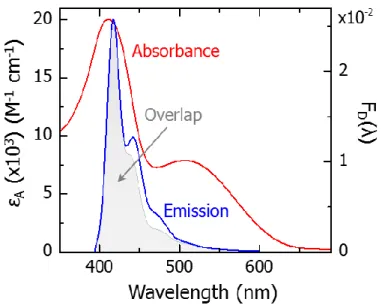
Figure 1.6. Transient absorption spectra following primary excitation of the polymer backbone at 388 nm for pF-Ru (upper left) and pT-Ru (upper right). (Bottom) RuII absorbance (εA(λ)) and normalized (to unit area) polymer emission spectra (FD(λ)). The shaded grey area reflects the integrand, FD(𝜆)𝜖𝐴(𝜆)𝜆4, which is scaled for clarity. (Right) Kinetic traces of the polymer
17
Table 1.1. Energy and electron transfer data for π-conjugated polymer assemblies with pendant RuII chromophores.
Energy Transfer Electron Transfer
Assembly
Energy Transfer: Electron Transfer
Ratio
τ (ps) τRET (ps) τ (ps) -ΔG 0
(eV) λ (eV)
pF-Ru 85:15 0.45 0.45 1.5 0.72
↑ 0.50-0.75
↓
pFT-Ru 75:25 0.7 1.2 2.0 0.45
pF2T-Ru 25:75 4.8 4.0 1.8 0.46
pT-Ru 15:85 8.1 10.0 1.1 0.50
The trend in energy transfer rates across the polymer series can be understood in terms of the absorption and emission properties of assemblies. The rate constant for resonant energy transfer (RET) between a donor (D) and acceptor (A) separated by a distance R is given by:
6 0 1 1 RET D R R
(1.2)
where 𝜏𝐷 is the excited-state lifetime of the donor, and 𝑅0 is the Förster distance, the distance at
which energy transfer is 50% efficient. The Förster distance can be estimated from independent spectroscopic measurements of the donor and acceptor according to:
06 2 0
4
)
( ( ) d
D D A
R A F
(1.3)where D is the quantum yield of the donor in the absence of the acceptor, and is a factor describing the relative orientations of the donor and acceptor The constant A is given by A=9000(ln 10)/(1285n4N
A), where n is the refractive index and NA is Avogadro’s number. The integral in Eq. 1.3 describes the product of the emission spectrum of the donor normalized to unity area and the absorption spectrum of the acceptor, as illustrated in Figure 1.6.
18
quantum yield of pF*. The decrease in the energy transfer rate across the series is attributed to a systematic shift in the emission spectrum to lower energy with increasing thiophene content, which results in an overall decrease in the overlap between the donor emission and acceptor absorption, as well as a decrease in the quantum yield of the polymer (ΦD). Energy transfer rates predicted
using Eq. 1.2 are in good agreement with the experimentally observed values (Table 1).46-48
The lifetimes of the charge-separated state produced by electron transfer also depends upon the polymer backbone. While the charge-separated state in pF-Ru undergoes recombination (i.e. back electron transfer) to reform the ground state with =6 ns, in pT-Ru it decays with 20 μs. The dramatic difference between these two assemblies may be a consequence of the high hole mobility of the pT polymer backbone, which could quickly and efficiently separate the electron and the hole.
19 1.3.4 Multifunctional Behavior
The eventual utilization of molecular assemblies in artificial photosynthetic applications will require that they perform multiple functions, including light-harvesting and charge separation, as well as storage and transport of redox equivalents to catalytic sites. Multifunctional behavior is observed in the excited-state photophysics of pS-Ru (Chapter 4) and pF-Ru (Chapter 5) assemblies anchored to TiO2 through carboxylate groups placed on 100% of the RuII complexes in pS-Ru and
30% of the Ru complexes in pF-Ru.50 The result is a composite structure, in which the assembly
is attached to the surface through a few complexes, while the remaining chromophores serve as antennas for light absorption and excited-state transport.
The photophysics of these assemblies on TiO2 were studied across 9 decades of time using
transient absorption spectroscopy (TA) and time-resolved emission spectroscopy (TRES). Photoexcitation of surface-bound RuII sites results in prompt electron injection into the TiO
2
conduction band, producing a RuIII species at the surface. In both pS-Ru and pF-Ru, site-to-site
energy transport is observed, where delayed electron injection on the ns time scale is observed, revealing the antenna nature of these assemblies to transport the excited-state energy to the surface Following electron injection in pS-Ru, the hole on the surface-bound RuIII complex is transferred
to the RuII sites away from the metal oxide surface, giving rise to a long-lived charge-separated
20
REFERENCES
1. Renger, G., Oxidative Photosynthetic Water Splitting: Energetics, Kinetics and Mechanism. Photosynth Res 2007, 91, 186-186.
2. Ferreira, K. N.; Iverson, T. M.; Maghlaoui, K.; Barber, J.; Iwata, S., Architecture of the Photosynthetic Oxygen-Evolving Center. Science 2004, 303, 1831-1838.
3. House, R. L.; Iha, N. Y. M.; Coppo, R. L.; Alibabaei, L.; Sherman, B. D.; Kang, P.; Brennaman, M. K.; Hoertz, P. G.; Meyer, T. J., Artificial Photosynthesis: Where Are We Now? Where Can We Go? J Photoch Photobio C 2015, 25, 32-45.
4. Meyer, T. J., Chemical Approaches to Artificial Photosynthesis. Accounts Chem Res 1989,
22, 163-170.
5. Alstrum-Acevedo, J. H.; Brennaman, M. K.; Meyer, T. J., Chemical Approaches to Artificial Photosynthesis. 2. Inorg Chem 2005, 44, 6802-6827.
6. Song, W. J.; Chen, Z. F.; Brennaman, M. K.; Concepcion, J. J.; Patrocinio, A. O. T.; Iha, N. Y. M.; Meyer, T. J., Making Solar Fuels by Artificial Photosynthesis. Pure Appl Chem 2011,
83, 749-768.
7. Treadway, J. A.; Moss, J. A.; Meyer, T. J., Visible Region Photooxidation on Tio2 with a Chromophore-Catalyst Molecular Assembly. Inorg Chem 1999, 38, 4386.
8. Gerischer, H., Photocatalysis in Aqueous-Solution with Small Tio2 Particles and the Dependence of the Quantum Yield on Particle-Size and Light-Intensity. Electrochim Acta 1995,
40, 1277-1281.
9. Gerischer, H., Photoelectrochemical Catalysis of the Oxidation of Organic-Molecules by Oxygen on Small Semiconductor Particles with Tio2 as an Example. Electrochim Acta 1993, 38, 3-9.
10. Ashford, D. L.; Gish, M. K.; Vannucci, A. K.; Brennaman, M. K.; Templeton, J. L.; Papanikolas, J. M.; Meyer, T. J., Molecular Chromophore-Catalyst Assemblies for Solar Fuel Applications. Chem Rev 2015, 115, 13006-13049.
11. Concepcion, J. J.; Jurss, J. W.; Brennaman, M. K.; Hoertz, P. G.; Patrocinio, A. O. T.; Iha, N. Y. M.; Templeton, J. L.; Meyer, T. J., Making Oxygen with Ruthenium Complexes. Accounts
Chem Res 2009, 42, 1954-1965.
12. Gust, D.; Moore, T. A.; Moore, A. L., Mimicking Photosynthetic Solar Energy Transduction. Accounts Chem Res 2001, 34, 40-48.
13. Sykora, M.; Maxwell, K. A.; DeSimone, J. M.; Meyer, T. J., Mimicking the Antenna-Electron Transfer Properties of Photosynthesis. Proceedings of the National Academy of Sciences
21
14. Fleming, C. N.; Maxwell, K. A.; DeSimone, J. M.; Meyer, T. J.; Papanikolas, J. M., Ultrafast Excited-State Energy Migration Dynamics in an Efficient Light-Harvesting Antenna Polymer Based on Ru(II) and Os(II) Polypyridyl Complexes. J Am Chem Soc 2001, 123, 10336-10347.
15. Fang, Z.; Ito, A.; Stuartt, A. C.; Luo, H. L.; Chen, Z. F.; Vinodgopal, K.; You, W.; Meyer, T. J.; Taylor, D. K., Soluble Reduced Graphene Oxide Sheets Grafted with Polypyridylruthenium-Derivatized Polystyrene Brushes as Light Harvesting Antenna for Photovoltaic Applications. Acs
Nano 2013, 7, 7992-8002.
16. Devadoss, C.; Bharathi, P.; Moore, J. S., Energy Transfer in Dendritic Macromolecules: Molecular Size Effects and the Role of an Energy Gradient. J Am Chem Soc 1996, 118, 9635-9644.
17. Balzani, V.; Campagna, S.; Denti, G.; Juris, A.; Serroni, S.; Venturi, M., Designing Dendrimers Based on Transition Metal Complexes. Light-Harvesting Properties and Predetermined Redox Patterns. Accounts Chem Res 1998, 31, 26-34.
18. Nantalaksakul, A.; Reddy, D. R.; Bardeen, C. J.; Thayumanavan, S., Light Harvesting Dendrimers. Photosynth Res 2006, 87, 133-150.
19. McCafferty, D. G.; Friesen, D. A.; Danielson, E.; Wall, C. G.; Saderholm, M. J.; Erickson, B. W.; Meyer, T. J., Photochemical Energy Conversion in a Helical Oligoproline Assembly.
Proceedings of the National Academy of Sciences of the United States of America 1996, 93,
8200-8204.
20. Knorr, A.; Galoppini, E.; Fox, M. A., Photoinduced Intramolecular Electron Transfer in Dichromophore-Appended Alpha-Helical Peptides: Spectroscopic Properties and Preferred Conformations. J Phys Org Chem 1997, 10, 484-498.
21. Serron, S. A.; Aldridge, W. S.; Fleming, C. N.; Danell, R. M.; Baik, M. H.; Sykora, M.; Dattelbaum, D. M.; Meyer, T. J., Evidence for through-Space Electron Transfer in the Distance Dependence of Normal and Inverted Electron Transfer in Oligoproline Arrays. J Am Chem Soc
2004, 126, 14506-14514.
22. Wilger, D. J.; Bettis, S. E.; Materese, C. K.; Minakova, M.; Papoian, G. A.; Papanikolas, J. M.; Waters, M. L., Tunable Energy Transfer Rates Via Control of Primary, Secondary, and Tertiary Structure of a Coiled Coil Peptide Scaffold. Inorg Chem 2012, 51, 11324-11338.
23. Bettis, S. E.; Ryan, D. M.; Gish, M. K.; Alibabaei, L.; Meyer, T. J.; Waters, M. L.; Papanikolas, J. M., Photophysical Characterization of a Helical Peptide Chromophore–Water Oxidation Catalyst Assembly on a Semiconductor Surface Using Ultrafast Spectroscopy. The
Journal of Physical Chemistry C 2014, 118, 6029-6037.