On the production and transfer of entangled electrons and photons

(1)

On the production and transfer

of entangled electrons and

photons

(2)

(3)

On the production and transfer of

entangled electrons and photons

PROEFSCHRIFT

ter verkrijging van

de graad vanDoctor aan deUniversiteitLeiden, op gezag van deRectorMagnificusDr. D. D. Breimer,

hoogleraar in de faculteit derWiskunde en Natuurwetenschappen en die derGeneeskunde, volgens besluit van hetCollege voorPromoties

te verdedigen op woensdag 28 september 2005 te klokke 15.15 uur

door

Joris Lodewijk van Velsen

(4)

Promotiecommissie:

Promotor: Prof. dr. C. W. J. Beenakker Referent: Prof. dr. J. P. Woerdman Overige leden: Prof. dr. P. H. Kes

Prof. dr. G. Nienhuis dr. L. M. K. Vandersypen

Het onderzoek beschreven in dit proefschrift is onderdeel van het wetenschap-pelijke programma van de Stichting voor Fundamenteel Onderzoek der Materie (FOM) en de Nederlandse Organisatie voor Wetenschappelijk Onderzoek (NWO).

(5)

(6)

(7)

Chapter 1 Introduction

The nonclassical correlation known as entanglement is one of the most counter-intuitive features of quantum mechanics and plays a central role in the emerging field of quantum computing and quantum information processing [1]. Two spa-tially separated particles are entangled if their joint state can not be prepared by operating on each particle separately — not even with the exchange of classical bits of information.

Entanglement is called a “resource” because it is both precious and useful: It isprecious, because if the quantum correlation is lost after the particles have been separated, it can not be restored without bringing them back together. It is useful, because entangled pairs of particles enable the disembodied transfer (= teleportation) of quantum bits of information (= qubits), which is a basic step in quantum algorithms.

The two separate aspects of entanglement production and transfer studied in this thesis were motivated by two separate lines of experimental research. For the entanglement transfer, we were motivated by an experiment in Leiden on the transmission of entangled photons through strongly scattering metal plates [2]. We have developed a general scattering theory of entanglement transfer that accounts for the highly entangled transmitted photons in the experiment.

For the entanglementproduction, our motivation came from experiments in progress in Delft to produce and detect entangled electrons trapped in quantum dots [3]. These experiments require control over the electron-electron interactions on short distances, first to entangle the electrons and then to spatially separate them. As described in this thesis, we came up with an alternative scheme for entanglement production and detection withfreeelectrons, that does not rely on electron-electron interactions.

(10)

2 CHAPTER 1. INTRODUCTION

The present chapter contains some background material on entanglement in general, and specifically on entanglement of electrons and photons.

1.1 Entanglement

The elementary entangled state is the spin singlet

|Bell =

1 √ 2

|↑A|↓B− |↓A|↑B

, (1.1)

also known as a Bell state. The indicesA,Blabel two spatially separated particles and the arrows ↑, ↓ indicate two spin states. The Bell state (1.1) can not be created by local operations and classical communication, because it is not known, not even in principle, which particle carries which spin. This is in contrast to the nonentangled mixed state with density matrix

ρmixed=

1 2

|↑↑|A⊗

|↓↓|B+

1 2

|↓↓|A⊗

|↑↑|B. (1.2)

The stateρmixed can be created by tossing with a coin: heads means Ais↑and

Bis↓, while tails means Ais↓andB is↑. By exchanging classical bits (heads or tails) and then locally rotating the spin, an ensemble described by ρmixed is

prepared.

1.1.1 Bell inequality

The spins in the state|Bellare correlated; a measurement of one spin, say with

outcome↑, projects the other spin on the opposite spin state↓. The same applies toρmixed. The difference between the correlation of the pure entangled state (1.1)

and the correlation of the mixed nonentangled state (1.2) is that the former persists if we measure the spin along a different axis, while the latter is diminished. For example, the change of basis

|↑ →√1 2

|↑ + |↓, |↓ →√1

2

|↑ − |↓ (1.3)

(both for spinAand spinB) leaves|Bellinvariant, butρmixedbecomes a mixture

of parallel and anti-parallel spins.

(11)

1.1. ENTANGLEMENT 3

performed on one particle, no information concerning the definite outcome of an experiment is transmitted to the other particle without classical communication on the choice of spin direction and the measurement result.

The correlations of nonentangled states can be described by classical mechan-ics in terms of the local and realistic theory (LRT) of EPR [4]. The correlation of the entangled state (1.1), however, goes beyond the LRT. This was demonstrated by Bell [5], who derived an inequality which is satisfied by the classical correla-tions of nonentangled states, but can be violated by the quantum correlacorrela-tions of entangled states.

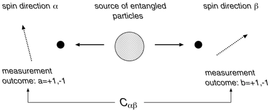
spin direction α source of entangled particles

spin direction β

measurement outcome: a=+1,-1

measurement outcome: b=+1,-1

C

_αβ

Figure 1.1: Scheme to detect entanglement by violation of the Bell inequality.

To explain the Bell inequality, we consider the setup indicated in Fig. 1.1. It consists of a source producing a pair of particles in the Bell state. Two lo-cal observers A and B each have a particle at their disposal. Within the LRT, measurement results can not depend on the choice of measurement of another spatially separated observer (locality) and the results of any measurement are pre-determined, regardless of whether the measurement is carried out or not (realism). Observers A and B each measure their spin along directionsαααandβββ with out-comea= ±1 andb= ±1, respectively. The correlator of the LRT is

Cαβαβαβ=

λ

p(λ)a(ααα,λ)b(βββ,λ). (1.4)

The “hidden” variable λ, with probability p(λ) in the ensemble, predetermines the measurement outcomes. By averaging the identity

(12)

over the ensemble of hidden variables, one obtains for the LRT the Clauser-Horne-Shimony-Holt (CHSH) form of the Bell inequality [6],

E=C_αβαβαβ+Cαβ_αβ_αβ+C_α_α_α_β_β_β−C_α_α_α_β_β_β≤2. (1.6)

In quantum mechanics the correlatorC_αβ_αβ_αβis given, instead of by Eq. (1.4), by the expectation value

Cαβαβαβ= (ααα·σσσ)A⊗(βββ·σσσ)B. (1.7) Hereσσσ =(σx,σy,σz) is the vector of Pauli matrices

σx=

0 1

1 0

, σy=

0 −i

i 0

, σz=

1 0

0 −1

. (1.8)

If Eq. (1.7) is inserted into Eq. (1.6) one finds that this inequality can be violated for certain states. These states can therefore not be described by the LRT, but must be described quantum mechanically.

All nonentangled states obey the Bell-CHSH inequality. IfE >2 for some choice of unit vectorsααα,ααα,βββ,βββ, then the spins are entangled. The converse of this statement is not true: There exist mixed states that are entangled and satisfy

E≤2 for all sets of unit vectors (see Sec. 1.1.3). The pure Bell state (1.1) has correlatorC_αβ_αβ_αβ= −ααα·βββand allows for the largest possible violationE=2√2>2 of the Bell-CHSH inequality.

1.1.2 Entanglement measures for pure states

An arbitrary pure state|in the bipartite Hilbert spaceH=HA⊗HB of a pair of two-level systems (= qubits) takes the form

| =

2

i=1 2

j=1

ci j|iA|jB, Trc†c=1. (1.9)

The basis states|1,|2may refer to spins (electrons), polarizations (photons), or other degrees of freedom.

Since an entangled state can not be prepared locally, one needs to exchange a certain amount of quantum information to create it out of a product state. This quantum information can take the form of Bell pairs (1.1), shared betweenAand B. Bell pairs play the role of a “currency”, by means of which one can quantify entanglement. The average number of Bell pairs per copy needed to prepare a large number of copies of the pure state|is given by [7]

(13)

1.1. ENTANGLEMENT 5

(The reduced density matrix ρA of subsystem A is obtained by tracing out the degrees of freedom of subsystem B.)

The quantityE∈[0, 1] is called the entanglement entropy, or entanglement of formation. In terms of the 2×2 matrix of coefficientsc, it takes the form

E=F

₁

2+ 1 2

1−4 Detc†_c _, _(1.11)

where the functionF(x) is defined by

F(x)= −xlog₂x−(1−x) log₂(1−x). (1.12)

The concurrenceC∈[0, 1] is in one-to-one relation withE but has a somewhat simpler expression:

C=2√Detc†_c. _(1.13)

A Bell pair has unit concurrence and entanglement of formation, while both C and Evanish for a product state.

For a pure state, the degree by which the Bell-CHSH inequality can be vio-lated is in one-to-one relation to the concurrenceC. By maximizing the correlator

Emax= max

ααα,βββ,ααα,βββ

C_αβ_αβ_αβ+C_αβ_αβ_αβ+C_α_α_α_β_β_β−C_α_α_α_β_β_β (1.14)

over four unit vectors, one obtains the Bell-CHSH parameterEmax. The relation

betweenEmaxandCis [8]

Emax=2

1+C2_. _(1.15)

The Bell-CHSH parameterEmaxranges from 2 to 2

√

2 as the concurrence ranges from 0 to 1.

1.1.3 Entanglement measures for mixed states

The density matrixρ of a mixed state can be decomposed into pure states|n with positive weight pn,

ρ=

n

pn|nn|, pn>0,

n

pn=1. (1.16)

The states|nare normalized to unity,n|n =1, but they need not be orthog-onal. The convex-sum decomposition is therefore not unique — there are many equivalent representations ofρas a mixture of pure states.

(14)

E= min

{n,pn}

n

pnE(n). (1.17)

Here E(n) is the entanglement entropy of the pure state|n, defined in Eq. (1.10), and the minimum is taken over all convex-sum decompositions ofρ. The entanglement of formationEhas a closed form expression given by [10]

E=F

₁

2+ 1 2

1−C2 _, _(1.18)

C=max

0,λ1−

λ2−

λ3−

λ4 . (1.19)

Theλi’s are the eigenvalues of the matrix productρ(σy⊗σy)ρ∗(σy⊗σy), in the orderλ1≥λ2≥λ3≥λ4. The quantityCis again called the concurrence. For a

pure state (withρ2₌_ρ_{) the definition (1.19) of}_C_{is equivalent to Eq. (1.13).}

The Bell-CHSH parameterEmaxfor an arbitrary mixed state of two qubits was

analyzed in Refs. [11, 12]. Unlike for a pure state, for a mixed state there is no one-to-one relation betweenC andEmax. Depending on the density matrix,Emax

can take on values between 2C√2 and 2√1+C2_{. The dependence of}E

maxonρ

involves the two largest eigenvaluesu1andu2of the real symmetric 3×3 matrix

RTR constructed from Rkl=Trρ σk⊗σl, whereσ1=σx,σ2=σy, andσ3=σz. The relation is

Emax=2

√

u1+u2. (1.20)

Violation of the Bell-CHSH inequality (Emax>2) impliesC>0, but not the other

way around. That is, there exist entangled mixed states (C>0) that can not violate the Bell-CHSH inequality (Emax≤2).

1.2 How to entangle photons

To produce entangled photons one can distinguish methods which rely on inter-actions between the photons (nonlinear optics) and methods which do not need interactions (linear optics).

1.2.1 Nonlinear optics

(15)

1.2. HOW TO ENTANGLE PHOTONS 7

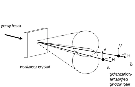
is indicated schematically in Fig. 1.2. A single pump photon of frequency 2ω is converted into two photons of frequency ω in different cones of orthogonal polarizations H and V. By collecting photons only along the two intersections of the cones, it is not known, not even in principle, which photon carries which polarization. This corresponds to the maximally entangled two-photon state

| =√1 2

|HA|VB+eiφ|VA|HB

. (1.21)

pump laser

nonlinear crystal

polarization-entangled photon pair

V

H H

V

A B

Figure 1.2: Scheme to create polarization-entangled photons by means of para-metric down-conversion.

1.2.2 Linear optics

A linear optical way of entangling photons is by means of elastic scattering at a beam splitter, see Fig. 1.3. A necessary condition for entanglement by linear optics is the nonclassicality of the photon sources: If the photons are incident in photon number (Fock) states or squeezed states, their polarizations can be entan-gled by a beam splitter [14]. However, classical states (such as thermal states or coherent states) can not be entangled. For a proof of this “no-go theorem”, we follow Ref. [15].

(16)

D_A D_B

beam splitter

S_B S_A

sources detectors

Figure 1.3: Scheme of entanglement production by a beam splitter.

the beam splitter can be written in the coherent state representation

ρin=

dαααP(ααα)|αααααα|, |ααα =eaaa†·ααα−aaa·ααα∗|0. (1.22)

The coherent state|ααα = |α1,α2,... is an eigenstate of the annihilation

opera-toran with complex eigenvalueαn. (The mode index n labels frequencies and polarizations of modes to the left and the right of the beam splitter.) We have ab-breviateddααα=ndReαndImαn. The real function P(ααα) may take on negative values. In that case the stateρin is called nonclassical, because P(ααα) can not be

interpreted as a classical distribution. A thermal state is a classical state with a GaussianP(ααα)∝exp(−_n|αn|2/fn), where fnis the Bose-Einstein distribution. The beam splitter transforms the annihilation operatorsaaa= {a1,a2,...}of the

incoming state into annihilation operatorsbbb= {b1,b2,...} of the outgoing state.

This is a unitary transformation,

bn=

m

Snmam, S S†=11, (1.23)

defined by the scattering matrixS. The density matrixρoutof the outgoing state

is obtained fromρinwith the help of Eq. (1.23). The result is

ρout=

dβββP(S†βββ)|ββββββ|, |βββ =ebbb†·βββ−bbb·βββ∗∗∗|0. (1.24)

(17)

1.3. HOW TO ENTANGLE ELECTRONS 9

are detected by Aand modes detected by B. Since the creation and annihilation operators of different modes commute, the pure state|βββis separable. It follows thatρoutis separable ifP≥0 for anyβββ, because in that case the density matrix has

a decomposition into separable pure states with positive weights. Nonclassicality is therefore a necessary condition for entangling photons at a beam splitter.

Even if we start from a nonclassical state, such as a two-photon Fock state, it is not garanteed that the beam splitter will produce entanglement. If, for instance, the two single photons are incident in wavepackets that are not timed to “collide” at the beam splitter, then their polarizations do not get entangled. This is because the photons are distinguishable by their temporal degrees of freedom.

1.3 How to entangle electrons

1.3.1 Interacting particles

Whereas violation of the Bell inequality has been demonstrated with photons [16], a similar achievement is still missing for electrons in the solid state. This may seem surprising, since entanglement in the solid state is the rule rather than the exception. The essential problem, however, lies in the controllable and coherent extraction of an entangled pair of electrons into two spatially separated conduc-tors.

There have been a number of theoretical proposals for solid-state entanglers. These schemes rely on interactions, such as the Coulomb interaction in a quantum dot [17–20] or the pairing interaction in a superconductor [21–23]. Two examples of these proposals are indicated schematically in Fig. 1.4.

1.3.2 Free particles

In this thesis, we propose an entangler for free electron-hole excitations, where both entanglement generation as well as spatial separation are realized purely by elastic scattering. The proposal in its simplest form consists of a single-channel conductor separated in two regions by a tunnel barrier. Incoming states to the right of the barrier are filled up to the Fermi energy EF, while the states to the

left are filled up to EF+eV (see Fig. 1.5). Tunneling of an electron across the

barrier produces an entangled electron-hole excitation |. If the tunneling is spin-independent, the spins of electron and hole are maximally entangled in the state

| =√1 2

|↑e|↑h+ |↓e|↓h

(18)

(a)

quantum

dot

(b)

SC

NT

V

_B A

I

A

B

A

B

I

δ

γ

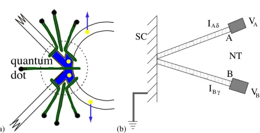
Figure 1.4: Solid-state entanglers making use of interactions. (a) Two coupled quantum dots with a single excess electron in each dot. The electron-pair is in its ground state, the entangled spin singlet state|Bell. Spatial separation is due

to strong on-site Coulomb repulsion (like in a hydrogen molecule). Mobile spin-entangled electrons are created by simultaneously lowering the tunnel barriers coupling each dot to separate leads. Picture by L. P. Kouwenhoven. (b) Two nanotubes (NT) are connected to a superconductor (SC). Each nanotube extracts an electron from a Cooper pair, generating spin-entangled currentsIAδ (δ=↑,↓)

andIBγ (γ =↑,↓) in the separate tubes A and B, respectively. Picture taken from

Ref. [23].

Electron-hole pairs are entangled even if the electron reservoirs are in thermal equilibrium at temperaturek T eV. This is in contrast to the linear optics en-tanglement by a beam splitter, which does not work if the sources are in thermal equilibrium. The Fermi sea, while being in local equilibrium, works around the optical no-go theorem described in Sec. 1.2.2.

(19)

entan-1.3. HOW TO ENTANGLE ELECTRONS 11

electron hole

Fermi sea

energy

position

barrier

E + eV_F

E_F

Figure 1.5: Schematic drawing of the electron-hole entangler proposed in this thesis. Tunneling events give rise to nonlocal spin correlations that can violate the Bell inequality.

(20)

nonlinear crystal pump laser

polarization-entangled photon pair

polarization-entangled photon pair synchronized

single-photon sources

beam splitter

V

metal

tunnel barrier (insulator)

spin-entangled electron-hole pair metal

voltage source

Figure 1.6: Schematic illustration of the entanglement of electron-hole pairs by a tunnel barrier and of photons by a nonlinear crystal and a beam splitter.

1.4 This thesis

Chapter 2: Production and detection of entangled electron-hole pairs in a degenerate electron gas

(21)

1.4. THIS THESIS 13

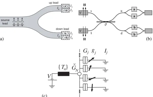
(a)

I₁ I₃ I_u

I_d I2

I₄

source lead

up lead

down lead

a

b V s

H

V

H

s u

a a

d

b

(b)

(c)

I

j

{ }

T

_n

V

G

_N

g

_j

G

j

Figure 1.7: Three geometries to produce and detect spin-entanglement in a normal conductor with ferromagnetic contacts. Panels a, b, and c are taken, respectively, from Refs. [25], [26], and [27].

schematically in Figs. 1.7 and 1.8.

Chapter 3: Dephasing of entangled electron-hole pairs in a degenerate electron gas

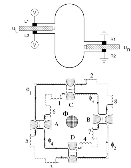
We continue our investigation of the electron-hole entangler, to include the ef-fects of dephasing. Dephasing appears because the electron and hole are coupled to other particles such as phonons and other electrons. Tracing out these other degrees of freedom corresponds to a transition from a pure electron-hole pair to a mixture. In this chapter, we investigate the loss of electron-hole entanglement due to this transition. Both the maximal violationEmaxof the Bell-CHSH inequality

(22)

(a)

V V

L1

L2

R1

R2 U

L

U R

(b)

φ

1

2

6

5

7

8

3

4

1

2 3

4

A

B

C

D

Φ

φ

(23)

1.4. THIS THESIS 15

Chapter 4: Scattering theory of plasmon-assisted entanglement trans-fer and distillation

We now turn from electrons to photons. In chapter 4, the quantum mechanical limits to the plasmon-assisted entanglement transfer observed in [2] are analyzed. The experimental setup is indicated schematically in Fig. 1.9. It consists of a non-linear crystal generating a pair of polarization-entangled photons. Subsequently, each photon passes through a metal plate perforated with arrays of holes smaller than the photon wavelength. On the metal plates, the entangled photons are each transformed into electron vibrations, called surface plasmons. The re-emitted photons are found to be still highly entangled. This signifies that after emission of a photon, the metal plate from which it originates does not carry information about its polarization. A scattering theory of entanglement transfer is constructed accordingly. This involves coherentscattering, turning a pure state into a pure state. (This is in contrast to the dephasing studied in chapter 3, which corresponds toincoherentor inelastic scattering, turning a pure state into a mixed state.) We find that the polarization-entanglement of a scattered photon pair can be described by two ratio’sτ1,τ2of polarization-dependent transmission probabilities. A fully

entangled incident state is transferred without degradation forτ1=τ2, but a

rel-atively large mismatch of τ1 and τ2 can be tolerated with a small reduction of

entanglement. We also predict that fully entangled Bell pairs can be distilled out of partially entangled radiation ifτ1andτ2satisfy a pair of inequalities.

perforated metal plate

polarization-entangled photon pair pump laser

nonlinear crystal

detector

coincidence counter polarizer

&

(24)

Chapter 5: Transition from pure-state to mixed-state entanglement by random scattering

We continue our analysis of chapter 4 on the transfer of polarization-entanglement, to include the effect of multi-mode detection. Although the scattering is elastic and the scattered state pure, the observed two-photon polarization-state is gen-erally mixed. This mixedness comes from the multi-mode detection, not from inelastic scattering like in chapter 3. Instead of the perforated metal plates of chapter 4, we consider scattering by disorder. Random matrix theory, applicable to disordered samples, allows us to find universal results — independent of mi-croscopic details. Entanglement of the detected polarization-state is quantified by the concurrenceC and maximal value of the Bell-CHSH parameterEmax. Both

these quantities decay exponentially with the number of detected modes in case that the scattering mixes the polarization directions and algebraically if it does not.

Chapter 6: Entangling ability of a beam splitter in the presence of tem-poral which-path information

(25)

Bibliography

[1] M. A. Nielsen and I. L. Chuang,Quantum Computation and Quantum In-formation(Cambridge University Press, Cambridge, 2000).

[2] E. Altewischer, M. P. van Exter, and J. P. Woerdman, Nature 418, 304 (2002).

[3] J. M. Elzerman, R. Hanson, L. H. Willems van Beveren, L. M. K. Van-dersypen, and L. P. Kouwenhoven, inQuantum Computation in Solid State Systems, edited by P. Delsing, C. Granata, Y. Pashkin, B. Ruggiero, and P. Silvestrini (Springer, Berlin, 2006).

[4] A. Einstein, B. Podolsky, and N. Rosen, Phys. Rev.47, 777 (1935).

[5] J. S. Bell, Physics1, 195 (1964).

[6] J. F. Clauser, M. A. Horne, A. Shimony, and R. A. Holt, Phys. Rev. Lett.23, 880 (1969).

[7] C. H. Bennett, H. J. Bernstein, S. Popescu, and B. Schumacher, Phys. Rev. A53, 2046 (1996).

[8] N. Gisin, Phys. Lett. A154, 201 (1991).

[9] C. H. Bennett, D. P. DiVincenzo, J. A. Smolin, and W. K. Wootters, Phys. Rev. A54, 3824 (1996).

[10] W. K. Wootters, Phys. Rev. Lett.80, 2245 (1998).

[11] R. Horodecki, P. Horodecki, and M. Horodecki, Phys. Lett. A 200, 340 (1995).

[12] F. Verstraete and M. M. Wolf, Phys. Rev. Lett.89, 170401 (2002).

(26)

18 BIBLIOGRAPHY

[13] L. Mandel and E. Wolf, Optical Coherence and Quantum Optics (Cam-bridge University Press, Cam(Cam-bridge, 1995).

[14] M. S. Kim, W. Son, V. Bužek, and P. L. Knight, Phys. Rev. A65, 032323 (2002).

[15] W. Xiang-bin, Phys. Rev. A66, 024303 (2002).

[16] A. Aspect, P. Grangier, and G. Roger, Phys. Rev. Lett.47, 460 (1981).

[17] G. Burkard, D. Loss, and E. V. Sukhorukov, Phys. Rev. B61, 16303 (2000); D. Loss and E. V. Sukhorukov, Phys. Rev. Lett.84, 1035 (2000).

[18] W. D. Oliver, F. Yamaguchi, and Y. Yamamoto, Phys. Rev. Lett.88, 037901 (2002).

[19] D. S. Saraga and D. Loss, Phys. Rev. Lett.90, 166803 (2003).

[20] M. Blaauboer and D. P. DiVincenzo, cond-mat/0502060.

[21] G. B. Lesovik, T. Martin, and G. Blatter, Eur. Phys. J. B24, 287 (2001).

[22] P. Recher, E. V. Sukhorukov, and D. Loss, Phys. Rev. B63, 165314 (2001); P. Recher and D. Loss, Phys. Rev. B65, 165327 (2002).

[23] C. Bena, S. Vishveshwara, L. Balents, and M. P. A. Fisher, Phys. Rev. Lett.

89, 037901 (2002).

[24] C. W. J. Beenakker, C. Emary, M. Kindermann, and J. L. van Velsen, Phys. Rev. Lett.91, 147901 (2003).

[25] A. V. Lebedev, G. B. Lesovik, and G. Blatter, Phys. Rev. B 71, 045306 (2005).

[26] A. V. Lebedev, G. Blatter, C. W. J. Beenakker, and G. B. Lesovik, Phys. Rev. B69, 235312 (2004).

[27] A. Di Lorenzo and Yu. V. Nazarov, Phys. Rev. Lett.94, 210601 (2005).

[28] C. W. J. Beenakker, M. Kindermann, C. M. Marcus, and A. Yacoby, in Fun-damental Problems of Mesoscopic Physics, edited by I. V. Lerner, B.L. Alt-shuler, and Y. Gefen, NATO Science Series II. Vol. 154 (Kluwer, Dordrecht, 2004).

(27)

Chapter 2 Production and detection of

entangled electron-hole pairs in a

degenerate electron gas

The controlled production and detection of entangled particles is the first step on the road towards quantum information processing [1]. In optics this step was taken long ago [2], but in the solid state it remains an experimental challenge. A variety of methods to entangle electrons have been proposed, based on quite different physical mechanisms [3]. A common starting point is a spin-singlet electron pair produced by interactions, such as the Coulomb interaction in a quantum dot [4– 6], the pairing interaction in a superconductor [7–9], or Kondo scattering by a magnetic impurity [10]. A very recent proposal based on orbital entanglement also makes use of the superconducting pairing interaction [11].

It is known that photons can be entangled by means of linear optics using a beam splitter [12–14]. The electronic analogue would be an entangler that is based entirely on single-electron physics, without requiring interactions. But a direct analogy with optics fails: Electron reservoirs are in local thermal equilib-rium, while in optics a beam splitter is incapable of entangling photons from a thermal source [15]. That is why previous proposals [10,16] to entangle electrons by means of a beam splitter start from a two-electron Fock state, rather than a many-electron thermal state. To control the extraction of a single pair of electrons from an electron reservoir requires strong Coulomb interaction in a tightly con-fined area, such as a semiconductor quantum dot or carbon nanotube [3]. Indeed, it has been argued [17] that one can not entangle a spatially separated current of electrons from a normal (not-superconducting) source without recourse to

(28)

20 CHAPTER 2. PRODUCTION AND DETECTION OF ENTANGLED . . .

actions.

What we would like to propose here is an altogether different, interaction-free source of entangled quasiparticles in the solid state. The entanglement is not between electron pairs but between electron-hole pairs in a degenerate elec-tron gas. The entanglement and spatial separation are realized purely by elastic scattering at a tunnel barrier in a two-channel conductor. We quantify the degree of entanglement by calculating how much the current fluctuations violate a Bell inequality.

Any two-channel conductor containing a tunnel barrier could be used in prin-ciple for our purpose, and the analysis which follows applies generally. The par-ticular implementation described in Fig. 2.1 uses edge channel transport in the integer quantum Hall effect [18]. It has the advantage that the individual building blocks have already been realized experimentally for different purposes. If the two edge channels lie in the same Landau level, then the entanglement is between the spin degrees of freedom. Alternatively, if the spin degeneracy is not resolved by the Zeeman energy and the two edge channels lie in different Landau levels, then the entanglement is between the orbital degrees of freedom. The beam split-ter is formed by a split gate electrode, as in Ref. [19]. In Fig. 2.1 we show the case that the beam splitter is weakly transmitting and strongly reflecting, but it could also be the other way around. To analyze the Bell inequality an extra pair of gates mixes the orbital degrees of freedom of the outgoing states independently of the incoming states. (Alternatively, one could apply a local inhomogeneity in the magnetic field to mix the spin degrees of freedom.) Finally, the current in each edge channel can be measured separately by using their spatial separation, as in Ref. [20]. (Alternatively, one could use the ferromagnetic method to measure spin current described in Ref. [3].)

Electrons are incident on the beam splitter from the left in a rangeeV above the Fermi energyEF. (The states belowEF are all occupied at low temperatures, so they do not contribute to transport properties.) The incident state has the form

|in =

0<ε<eV

a†_in,1(ε)a†_in,2(ε)|0. (2.1)

(29)

21

UL

UR

1 2

1

2 V

B

S

(30)

matrix notation,

|in =

ε

a_in† b†_in

1

2σy 0

0 0

a_in† b†_in

|0, (2.2)

withσya Pauli matrix.

The input-output relation of the beam splitter is

aout bout = r t t r ain bin . (2.3)

The 4×4 unitary scattering matrixShas 2×2 submatricesr,r,t,tthat describe reflection and transmission of states incident from the left or from the right. Sub-stitution of Eq. (2.3) into Eq. (2.2) gives the outgoing state

|out =

ε

a†outrσytTbout† +[rσyrT]12a † out,1a

†

out,2+[tσytT]12b † out,1b

† out,2

|0. (2.4)

The superscript “T” indicates the transpose of a matrix.

To identify the entangled electron-hole excitations we transform from particle to hole operators at the left of the beam splitter:cout,i =aout,† i. The new vacuum state isa_out,1† a_out,2† |0. To leading order in the transmission matrix the outgoing state becomes

|out =

ε

√

w| +√1−w|0, (2.5)

| =w−1/2_c† outγb

†

out|0, γ =σyrσytT. (2.6)

It represents a superposition of the vacuum state and a particle-hole statewith weightw=Trγ γ†_.

The degree of entanglement ofis quantified by the concurrence [21, 22],

C=2Detγ γ†_/_Tr_{γ γ}†

, (2.7)

which ranges from 0 (no entanglement) to 1 (maximal entanglement). Substitut-ing Eq. (2.6) and usSubstitut-ing the unitarity of the scatterSubstitut-ing matrix we find after some algebra that

C=2 √

(1−T1)(1−T2)T1T2

T1+T2−2T1T2 ≈

2T1T2/(T1+T2) if T1,T21. (2.8)

The concurrence is entirely determined by the eigenvaluesT1,T2∈(0, 1) of the

(31)

23

Maximal entanglement is achieved if the two transmission eigenvalues are equal:

C=1 ifT1=T2.

The particle-hole entanglement is a nonlocal correlation that can be detected through the violation of a Bell inequality. We follow the formulation in terms of irreducible current correlators of Samuelsson, Sukhorukov, and Büttiker [11]. In the tunneling regime considered here that formulation is equivalent to the original formulation in terms of coincidence counting rates [23]. The tunneling assump-tion is essential: If T1,T2 are not 1 one can not violate the Bell inequality

without coincidence detection [17]. The quantityCi j =

_∞

−∞dtδIL,i(t)δIR,j(0) correlates the time-dependent cur-rent fluctuations δIL,i in channeli =1, 2 at the left with the current fluctuations δIR,j in channel j =1, 2 at the right. It can be measured directly in the fre-quency domain as the covariance of the low-frefre-quency component of the current fluctuations. At low temperatures (k T eV) the correlator has the general ex-pression [24]

Ci j = −(e3V/h)|(r t†)i j|2. (2.9)

We need the following rational function of correlators:

E=C11+C22−C12−C21 C11+C22+C12+C21

=Trσzr t†σztr†

Trr†_{r t}†_t . (2.10)

By mixing the channels locally in the left and right arm of the beam splitter, the transmission and reflection matrices are transformed asr →ULr,t →URt, with unitary 2×2 matricesUL,UR. The correlator transforms as

E(UL,UR)=

TrU_L†σzULr t†U

†

RσzURtr†

Trr†_{r t}†_t . (2.11)

The Bell-CHSH (Clauser-Horne-Shimony-Holt) parameter is [23, 25]

E=E(UL,UR)+E(UL,UR)+E(UL,UR)−E(UL,UR). (2.12)

The state is entangled if|E|>2 for some set of unitary matricesUL,UR,UL,UR. By repeating the calculation of Ref. [26] we find the maximum [27]

Emax=2[1+4T1T2(T1+T2)−2]1/2>2. (2.13)

Comparison with Eq. (2.8) confirms the expected relation Emax=2(1+C2)1/2

(32)

(33)

Bibliography

[1] B. M. Terhal, M. M. Wolf, and A. C. Doherty, Physics Today (April, 2003): p. 46.

[2] A. Aspect, P. Grangier, and G. Roger, Phys. Rev. Lett.47, 460 (1981).

[3] T. Martin, A. Crepieux, and N. Chtchelkatchev, inQuantum Noise in Meso-scopic Physics, edited by Yu. V. Nazarov, NATO Science Series II Vol. 97 (Kluwer, Dordrecht, 2003), p. 313; J. C. Egues, P. Recher, D. S. Saraga, V. N. Golovach, G. Burkard, E. V. Sukhorukov, and D. Loss,ibid., p. 241.

[4] G. Burkard, D. Loss, and E. V. Sukhorukov, Phys. Rev. B 61, R16303 (2000); D. Loss and E. V. Sukhorukov, Phys. Rev. Lett.84, 1035 (2000).

[5] W. D. Oliver, F. Yamaguchi, and Y. Yamamoto, Phys. Rev. Lett.88, 037901 (2002).

[6] D. S. Saraga and D. Loss, Phys. Rev. Lett.90, 166803 (2003).

[7] G. B. Lesovik, T. Martin, and G. Blatter, Eur. Phys. J. B24, 287 (2001).

[8] P. Recher, E. V. Sukhorukov, and D. Loss, Phys. Rev. B63, 165314 (2001); P. Recher and D. Loss, Phys. Rev. B65, 165327 (2002).

[9] C. Bena, S. Vishveshwara, L. Balents, and M. P. A. Fisher, Phys. Rev. Lett.

89, 037901 (2002).

[10] A. T. Costa, Jr. and S. Bose, Phys. Rev. Lett.87, 277901 (2001).

[11] P. Samuelsson, E. V. Sukhorukov, and M. Büttiker, Phys. Rev. Lett. 91, 157002 (2003).

[12] E. Knill, R. Laflamme, and G. J. Milburn, Nature409, 46 (2001).

(34)

26 BIBLIOGRAPHY

[13] S. Scheel and D.-G. Welsch, Phys. Rev. A64, 063811 (2001).

[14] M. S. Kim, W. Son, V. Bužek, and P. L. Knight, Phys. Rev. A65, 032323 (2002).

[15] W. Xiang-bin, Phys. Rev. A66, 024303 (2002).

[16] S. Bose and D. Home, Phys. Rev. Lett.88, 050401 (2002).

[17] N. M. Chtchelkatchev, G. Blatter, G. B. Lesovik, and T. Martin, Phys. Rev. B66, 161320(R) (2002).

[18] C. W. J. Beenakker and H. van Houten, Solid State Phys.44, 1 (1991).

[19] M. Henny, S. Oberholzer, C. Strunk, T. Heinzel, K. Ensslin, M. Holland, and C. Schönenberger, Science284, 296 (1999).

[20] B. J. van Wees, E. M. M. Willems, C. J. P. M. Harmans, C. W. J. Beenakker, H. van Houten, J. G. Williamson, C. T. Foxon, and J. J. Harris, Phys. Rev. Lett.62, 1181 (1989).

[22] The concurrence quantifies the entanglement per electron-hole pair. We have also calculated the entanglement of formationF (measured in bits per sec-ond) for the full stateoutin Eq. (2.4). We findF = −(eV/h)[T1logT1(1−

T2)+T2logT2(1−T1)+(1−T1−T2) log(1−T1)(1−T2)]. For T1,T21

this reduces toF ≈ −(eV/h)[T1logT1+T2logT2].

[23] J. S. Bell, Physics1, 195 (1964); J. F. Clauser, M. A. Horne, A. Shimony, and R. A. Holt, Phys. Rev. Lett.23, 880 (1969).

[24] M. Büttiker, Phys. Rev. Lett.65, 2901 (1990).

[25] Instead of searching for violations of the CHSH inequality |E| ≤2, one could equivalently consider the CH (Clauser-Horne) inequality ECH ≤

0, with ECH =(−e3V/h)−1{Ci j(UL,UR)+Ci j(U_L,UR)+Ci j(UL,U_R)− Ci j(UL,UR)−Ci1(UL,11)−Ci2(UL,11)−C1j(11,UR)−C2j(11,UR)}. Substi-tutingCi j(U,V)=(−e3V/h)|(U r t†V†)i j|2 one obtains the relationECH= 1

4(E−2)Trrr

†_tt†_{between the CH and CHSH parameters.}

(35)

BIBLIOGRAPHY 27

[27] The maximum (2.13) is attained forUR=X,UR =2−1/2(11+iσy)X,UL = (11 cosα+iσysinα)Y, U_L =(11 cosα−iσysinα)Y, with tan 2α=C. The unitary matricesX,Y are chosen such thatY r t†X†is real diagonal.

(36)

(37)

Chapter 3 Dephasing of entangled electron-hole

pairs in a degenerate electron gas

3.1 Introduction

The production and detection of entangled particles is the essence of quantum information processing [1]. In optics, this is well-established with polarization-entangled photon pairs, but in the solid state it remains an experimental challenge. There exist several theoretical proposals for the production and detection of en-tangled electrons [2, 3]. These theoretical works address mainly pure states. The purpose of this chapter is to investigate what happens if the state is mixed. Some aspects of this problem were also considered in Refs. [4, 5]. We go a bit further by comparing violation of the Bell inequality to the degree of entanglement of the mixed state.

The entanglement scheme that we will analyze here, proposed in chapter 2, involves the Landau level index of an electron and hole quasiparticle (see Fig. 2.1). We consider one specific mechanism for the loss of purity, namely inter-action with the environment. We model this interinter-action phenomenologically by introducing phase factors in the scattering matrix and subsequently averaging over these phases. A more microscopic treatment (for example along the lines of a re-cent paper [6]) is not attempted here. Another kind of mixture would result from energy averaging [7]. We assume that the applied voltage is sufficiently small that we can neglect energy averaging. Experimentally, both energy and phase averaging may play a role [8].

(38)

30 CHAPTER 3. DEPHASING OF ENTANGLED . . .

3.2 Dephasing

Dephasing is introduced phenomenologically through random phase shiftsφi (ψi) accumulated in channeli at the left (right) of the tunnel barrier. The reflection and transmission matricesrandt transform as

r →

eiφ1 ₀

0 eiφ2

r0, t→

eiψ1 ₀

0 eiψ2

t0. (3.1)

By averaging over the phase shifts, with distribution P(φ1,φ2,ψ1,ψ2), and

pro-jecting out the vacuum contribution, the pure electron-hole excitation is converted into a mixture described by a 4×4 density matrix

ρi j,kl=

γi jγkl∗

Trγ γ†. (3.2)

Here ··· denotes the average over the phases and the matrix γ refers to an electron-hole excitation cf. Eq. (2.6). The degree of entanglement is quantified by the concurrenceC, given by [9]

C=max0,λ1−

λ2−

λ3−

λ4

. (3.3)

Theλi’s are the eigenvalues of the matrix productρ·(σy⊗σy)·ρ∗·(σy⊗σy), in the orderλ1≥λ2≥λ3≥λ4. The concurrence ranges from 0 (no entanglement)

to 1 (maximal entanglement).

The entanglement of the particle-hole excitations is detected by the violation of the Bell-CHSH (Clauser-Horne-Shimony-Holt) inequality [10, 11]. This re-quires two gate electrodes to locally mix the edge channels (scattering matrices UL,UR) and two pairs of contacts 1, 2 to separately measure the current fluctua-tionsδIL,i andδIR,i (i =1, 2) in each transmitted and reflected edge channel. In the tunneling regime the Bell inequality can be formulated in terms of the low-frequency noise correlator [5]

Ci j=

_∞

−∞

dtδIL,i(t)δIR,j(0). (3.4)

At low temperatures (k T eV) the correlator has the general expression [12]

Ci j(UL,UR)= −(e3V/h)

ULr t†UR† i j

(39)

3.3. CALCULATION OF THE MIXED-STATE ENTANGLEMENT 31

We again introduce the random phase shifts intor andtand average the correlator. The Bell-CHSH parameter is

E= |E(UL,UR)+E(UL,UR)+E(UL,UR)−E(UL,UR)|, (3.6)

whereE(U,V) is related to the average correlatorsCi j(U,V)by

E=C11+C22−C12−C21 C11+C22+C12+C21

. (3.7)

The state is entangled ifE>2 for some set of 2×2 unitary matricesUL,UR,UL,UR. IfE=2√2 the entanglement is maximal.

3.3 Calculation of the mixed-state entanglement

We simplify the problem by assuming that the two transmission eigenvalues (eigen-values oftt†_{) are identical:} _T

1=T2≡T. In the absence of dephasing the

elec-tron and hole then form a maximally entangled pair. The transmission matrix t0=T1/2V and reflection matrix r0=(1−T)1/2V in this case are equal to a

scalar times a unitary matrixV,V. Any 2×2 unitary matrixcan be parame-terized by

=eiθ

eiα ₀ 0 e−iα

cosξ sinξ −sinξ cosξ

eiβ ₀ 0 e−iβ

, (3.8)

in terms of four real parametersα,β,θ,ξ. The angleξgoverns the extent to which

mixes the degrees of freedom (no mixing forξ =0,π/2, complete mixing for

ξ =π/4).

If we set=σyVσyVTwe obtain for the matrixγof Eq. (2.6) the parametriza-tion

γ =eiθT(1−T)

eiφ2+iα ₀

0 eiφ1−iα

eiψ1+iβ ₀

0 eiψ2−iβ

.

(3.9) In the same parametrization, the matrixr t†which appears in Eq. (3.5) takes the form

r t†=eiθ−iθT(1−T)× (3.10)

eiφ1−iα ₀

0 eiφ2+iα

e−iψ1−iβ ₀

0 e−iψ2+iβ

(40)

witheiθ ₌_Det_V_{. We have used the identity} _V_V†₌_(Det_V₎₍_σ

yVσyVT)∗ to relate the parametrization ofr t†to that ofγ. Note that

Trγ γ†=2T(1−T)=Trr t†tr†, (3.11)

independent of the phase shiftsφi andψi.

To average the phase factors we assume that the phase shifts at the left and the right of the tunnel barrier are independent, so

P(φ1,φ2,ψ1,ψ2)=PL(φ1,φ2)PR(ψ1,ψ2). (3.12)

The complex dephasing parametersηLandηRare defined by

ηL=

dφ1

dφ2PL(φ1,φ2)eiφ1−iφ2, ηR=

dψ1

dψ2PR(ψ1,ψ2)eiψ1−iψ2.

(3.13) The density matrix (3.2) of the mixed particle-hole state has, in the parametriza-tion (3.9), the elements

ρ=1 2

⎛ ⎜ ⎜ ⎝

cos2_ξ _η_˜

Rcosξsinξ −η˜∗Lcosξsinξ η˜∗Lη˜Rcos2ξ ˜

η∗

Rcosξsinξ sin

2_ξ ₋_η_˜∗

Lη˜∗Rsin

2_ξ _η_˜∗

Lcosξsinξ −η˜Lcosξsinξ −η˜Lη˜Rsin2ξ sin2ξ −η˜Rcosξsinξ

˜

ηLη˜∗Rcos2ξ η˜Lcosξsinξ −η˜∗Rcosξsinξ cos2ξ

⎞ ⎟ ⎟ ⎠.

(3.14) We have defined ˜ηL=ηLe−2iα, ˜ηR=ηRe2iβ. The concurrenceC, calculated from Eq. (3.3), has a complicated expression. For|ηL| = |ηR| ≡ηit simplifies to

C=max

0,−1 2(1−η

2₎₊1

4

16η2+₂₍₁−η2₎2₍₁+_{cos 4}ξ₎

. (3.15)

Notice thatC=η2_for_ξ ₌_0.

For the Bell inequality we first note that the ratio of correlators (3.7) can be written as

E(UL,UR)= 1

2T(1−T)TrU

†

LσzULr t

†

U_R†σzU_Rtr†. (3.16)

We parameterize

(41)

3.4. DISCUSSION 33

in terms of two unit vectors ˆnL, ˆnRand a vectorσ of Pauli matrices

σx=

0 1

1 0

≡σ1, σy=

0 −i

i 0

≡σ2, σz=

1 0

0 −1

≡σ3. (3.19)

Substituting the parametrization (3.10), Eq. (3.16) takes the form

E(UL,UR)= 1 2Tr

nL,z η˜∗Lν∗L ˜

ηLνL −nL,z

×

nR,z η˜∗Rν∗R ˜

ηRνR −nR,z

cosξ −sinξ sinξ cosξ

, (3.20)

where we have abbreviatedνL=nL,x+i nL,y,νR=nR,x+i nR,y. Comparing Eqs. (3.14) and (3.20), we see that

E(UL,UR)=Trρ( ˆnL· σ)T⊗( ˆnR· σ) . (3.21)

(The transpose appears because of the transformation from electron to hole op-erators at the left of the barrier.) This is an explicit demonstration that the noise correlator (3.7) measures the density matrix (3.2) of the projected electron-hole state — without the vacuum contribution.

The maximal valueEmaxof the Bell-CHSH parameter (3.6) for an arbitrary

mixed state was analyzed in Refs. [13, 14]. For a pure state with concurrenceC one has simply Emax=2

√

1+C2_{[15]. For a mixed state there is no one-to-one}

relation betweenEmaxandC. Depending on the density matrix,Emaxcan take on

values between 2C√2 and 2√1+C2_{. The general formula}

Emax=2

√

u1+u2 (3.22)

for the dependence of Emax on ρ involves the two largest eigenvalues u1,u2 of

the real symmetric 3×3 matrixRT_R_{constructed from}_R

kl=Trρ σk⊗σl. For our density matrix (3.14) we find from Eq. (3.22) a simple expression if|ηL| = |ηR| ≡ η. It reads

Emax=

√

2(1+η2₎2+₍₁−η2₎2_{cos 4}ξ_. _(3.23)

3.4 Discussion

The resultEmax=2(1+η4)1/2which follows from Eq. (3.23) forξ=0 was found

(42)

Figure 3.1: Relation between the maximal violationEmax of the Bell-CHSH

in-equality and the concurrenceCcalculated from Eqs. (3.15) and (3.23) for mixing parametersξ =0 (triangles, no mixing) andξ =π₄ (squares, complete mixing). The dephasing parameterη decreases from 1 (upper right corner, no dephasing) to 0 (lower left, complete dephasing) with steps of 0.05. The dotted line is the relation betweenEmax and C for a pure state, which is also the largest possible

value ofEmaxfor givenC.

Emax≤2 is then violated for arbitrarily strong dephasing. This is not true in the

more general caseξ=0, whenEmaxdrops below 2 at a finite value ofη.

In Fig. 3.1 we compareEmaxandCforξ=0 (no mixing) andξ=π₄ (complete

mixing). For ξ =0 the same relation Emax=2

√

1+C2 _between _E

max and C

holds as for pure states (dotted curve). Violation of the Bell inequality is then equivalent to entanglement. Forξ=0 there exist entangled states (C>0) without violation of the Bell inequality (Emax≤2). Violation of the Bell inequality is

then a sufficient but not a necessary condition for entanglement. We define two characteristic dephasing parametersη_E andη_Cby the smallest values such that

(43)

3.4. DISCUSSION 35

The numberη_E is the dephasing parameter below which Bell’s inequality cannot be violated; The dephasing parameterη_Cgives the border between entanglement and no entanglement. From Eqs. (3.15) and (3.23) we obtain

ηC=

5−cos 4ξ−2√2√3−cos 4ξ

1−cos 4ξ , ηE =

−1+cos 4ξ+√2−2 cos 4ξ

1+cos 4ξ .

(3.25) The two dephasing parameters are plotted in Fig. 3.2. The inequality η_E ≥η_C reflects the fact thatEmaxis an entanglement witness.

Figure 3.2: The Bell-CHSH inequality is violated for dephasing parameters

η > ηE, while entanglement is preserved for η > ηC. The shaded region

indi-cates dephasing and mixing parameters for which there is entanglement without violation of the Bell-CHSH inequality.

(44)

Bell states

|ψα =√1

2(|↑↓ +e i_α_|↓↑

), |φ_α = √1

2(|↑↑ +e i_α_|↓↓

). (3.26)

(45)

Bibliography

[1] M. A. Nielsen and I. L. Chuang,Quantum Computation and Quantum In-formation(Cambridge University Press, Cambridge, 2000).

[2] J. C. Egues, P. Recher, D. S. Saraga, V. N. Golovach, G. Burkard, E. V. Sukhorukov, and D. Loss, inQuantum Noise in Mesoscopic Physics, edited by Yu. V. Nazarov, NATO Science Series II Vol. 97 (Kluwer, Dordrecht, 2003).

[3] T. Martin, A. Crepieux, and N. Chtchelkatchev, inQuantum Noise in Meso-scopic Physics, edited by Yu. V. Nazarov, NATO Science Series II Vol. 97 (Kluwer, Dordrecht, 2003).

[4] G. Burkard and D. Loss, Phys. Rev. Lett. 91, 087903 (2003).

[5] P. Samuelsson, E. V. Sukhorukov, and M. Büttiker, Phys. Rev. Lett. 91, 157002 (2003).

[6] F. Marquardt and C. Bruder, Phys. Rev. Lett. 92, 056805 (2004).

[7] Referring to Fig. 2.1, consider the area A between the two equipotentials starting atUL, through S, and ending atUR. This enclosed area varies by δAwhen the energy of the equipotentials varies byeV. Dephasing results if BδAh/e. The ratioδA/AV|∇ E|/| E|2depends on the gradient of the electric field E near the edge. For B=5 T, A=10−13_m2_{, one would need}

V 10−2_|_E_|2_/_|∇_E_|_{to avoid dephasing by energy averaging.}

[8] Y. Ji, Y. Chung, D. Sprinzak, M. Heiblum, D. Mahalu, and H. Shtrikman, Nature422, 415 (2003).

[10] J. F. Clauser, M. A. Horne, A. Shimony, and R. A. Holt, Phys. Rev. Lett.23, 880 (1969).

(46)

38 BIBLIOGRAPHY

[11] N. M. Chtchelkatchev, G. Blatter, G. B. Lesovik, and T. Martin, Phys. Rev. B66, 161320(R) (2002).

[12] M. Büttiker, Phys. Rev. Lett.65, 2901 (1990).

[13] R. Horodecki, P. Horodecki, and M. Horodecki, Phys. Lett. A 200, 340 (1995).

[14] F. Verstraete and M. M. Wolf, Phys. Rev. Lett.89, 170401 (2002).

(47)

Chapter 4 Scattering theory of

plasmon-assisted entanglement

transfer and distillation

The motivation for the work presented in this chapter came from the remark-able demonstration by Altewischer, Van Exter, and Woerdman of the transfer of quantum mechanical entanglement from photons to surface plasmons and back to photons [1]. Since entanglement is a highly fragile property of a two-photon state, it came as a surprise that this property could survive with little degradation the conversion to and from the macroscopic degrees of freedom in a metal [2].

We present a quantitative description of the finding of Ref. [1] that the en-tanglement is lost if it is measured during transfer, that is to say, if the medium through which the pair of polarization-entangled photons is passed acts as a “which-way” detector for polarization. Our analysis explains why a few percent degradation of entanglement could be realized without requiring a highly sym-metric medium. We predict that the experimental setup of Ref. [1] could be used to “distill” [3, 4] fully entangled Bell pairs out of partially entangled incident ra-diation, and we identify the region in parameter space where this distillation is possible.

We assume that the medium islinear, so that its effect on the radiation can be described by a scattering matrix. The assumption of linearity of the interaction of radiation with surface plasmons is central to the literature on this topic [5–9]. We will not make any specific assumptions on the mode and frequency depen-dence of the scattering matrix, but extract the smallest number of independently measurable parameters needed to describe the experiment. By concentrating on

(48)

40 CHAPTER 4. SCATTERING THEORY OF . . .

model-independent results we can isolate the fundamental quantum mechanical limitations on the entanglement transfer, from the limitations specific for any par-ticular transfer mechanism.

The system considered is shown schematically in Fig. 4.1. Polarization-entangled radiation is scattered by two objects and detected by a pair of detec-tors behind the objects in the far-field. The objects used in Ref. [1] are metal films perforated by a square array of subwavelength holes. The transmission am-plitude t_{σ σ},i of object i =1, 2 relates the transmitted radiation (with polariza-tionσ =H, V) to the incident radiation (polarizationσ=H, V). We assume a single-mode incident beam and a single-mode detector (smaller than the coher-ence area), so that we require a set of eight transmission amplitudestσ σ,i out of the entire scattering matrix (which also contains reflection amplitudes and trans-mission amplitudes to other modes). We do not require that the scattering matrix is unitary, so our results remain valid if the objects absorb part of the incident radiation. What is neglected is the thermal radiation, either from the two objects or from the electromagnetic environment of the detectors. This thermal noise is insignificant at room temperature and optical frequencies.

The radiation incident on the two objects is in a known, partially entangled state and we wish to determine the degree of entanglement of the detected radia-tion. It is convenient to use a matrix notaradia-tion. The incident two-photon state has the general form

|in =ainHH|HH +a in

HV|HV +a in

VH|VH +a in

VV|VV. (4.1)

The four complex numbersain_{σ σ} form a matrix

Ain=

a_HHin a_HVin ain

VH aVVin

. (4.2)

Normalization of|inrequires TrA_inA†_in=1.

The four transmission amplitudest_{σ σ},i of objecti =1, 2 form the matrix

Ti=

tHH,i tHV,i tVH,i tVV,i

. (4.3)

The transmitted two-photon state|outhas matrix of coefficients

Aout=Z−1/2T1AinT2T, (4.4)

with normalization factor

Z =Tr (T1AinT2T) (T1AinT2T) †

(49)

41

&

1

2

Figure 4.1: Main plot: Efficiency of the entanglement transfer for a fully en-tangled incident state, as given by Eq. (4.13). The maximal violation Emax

of Bell’s inequality at the photodetectors is plotted as a function of the ratio

τ1/τ2=T1+T2−/T1−T2+of the polarization-dependent transmission probabilities.

The inset shows schematically the geometry of the experiment [1]. A pair of polarization-entangled photons is incident from the left on two perforated metal films. The photodetectors at the right, connected by a coincidence counter, mea-sure the degree of entanglement of the transmitted radiation.

For a pure state|the maximal value of the Bell-CHSH parameterEmax[10]

is related to the concurrenceC[11] byEmax=2

√

1+C2_{[12]. In terms of a matrix}

A, the concurrence takes the formC=2|DetA|and ranges from 0 (no entangle-ment) to 1 (maximal entangleentangle-ment). A fully entangled state could be the Bell pair

|HV − |VH/√2, or any state derived from it by a local unitary transformation (A→U AV withU,V arbitrary unitary matrices). The degree of entanglement

Cin=2|DetAin|of the incident state is given and we seek the degree of

entangle-mentCout=2|DetAout|of the transmitted state. We are particularly interested in

the largest Cout that can be reached by applying local unitary transformations to

On the production and transfer of entangled electrons and photons

On the production and transfer

of entangled electrons and

photons

On the production and transfer of

entangled electrons and photons

Joris Lodewijk van Velsen

Contents

Chapter 1

Introduction

1.1

Entanglement

C

1.2

How to entangle photons

1.3

How to entangle electrons

quantum

dot

SC

NT

V

V

I

A

B

I

1.4

This thesis

I

{ }

T

V

G

g

G

φ

1

2

6

5

7

8

3

4

A

B

C

D

Φ

φ

φ

φ

Bibliography

Chapter 2

Production and detection of

entangled electron-hole pairs in a

degenerate electron gas

Bibliography

Chapter 3

Dephasing of entangled electron-hole

pairs in a degenerate electron gas

3.1

Introduction

3.2

Dephasing

3.3

Calculation of the mixed-state entanglement

3.4

Discussion

Bibliography

Chapter 4

Scattering theory of

plasmon-assisted entanglement

transfer and distillation

&