Sharif University of Technology
Scientia IranicaTransactions A: Civil Engineering http://scientiairanica.sharif.edu
Optimal location of stone column for stabilization of
sand slope: An experimental and 3D numerical
investigation
M. Hajiazizi
, E. Nemati, M. Nasiri, M. Bavali, and M. Sharipour
Department of Civil Engineering, Razi University, Taq-e Bostan, Kermanshah, Iran.Received 22 July 2017; received in revised form 26 November 2017; accepted 23 April 2018
KEYWORDS Stabilization; Sand slope; Stone column; Optimal location; Experimental test.
Abstract.The subject of utilizing numerical and analytical methods for stabilizing earth slopes by applying piles or stone columns is commonly discussed by numerous researchers. Various researchers have attempted to optimize the location of pile or stone column to stabilize earth slope through numerical and analytical approaches. Their eorts have produced various results that raised the question of what the optimal place for installation of a pile or stone column is. It appears that no experimental studies are conducted in this regard: the point to be discussed in this article. Experimental study conducted in this article is a new topic and can solve the problem caused by varying and sometimes contradictory results of numerical analyses to nd the optimal pile (or stone column) location. In this article, an experimental study is conducted for a two-layer sand earth slope, which is saturated through precipitation and failure after saturation over time. By installing stone columns at dierent locations and saturating the earth slope through precipitation, rational and acceptable results were obtained that could appropriately assist designers. All of the experimental models were modeled and compared by the 3D nite dierence method (3D FDM), which are compliant with each other.
© 2020 Sharif University of Technology. All rights reserved.
1. Introduction
Stability analysis of earth slopes is one of the major issues raised in Geo-Engineering, which has attracted many researchers' attention from dierent parts of the world. When the stability of an earth slope is evaluated, it is necessary to take preventive measures before instability occurs. The rst action to maintain the stability of an earth slope is to perform excavation
*. Corresponding author.
E-mail addresses: mhazizi@razi.ac.ir (M. Hajiazizi); ismail.nemati@yahoo.com (E. Nemati);
nasiri.ma@razi.ac.ir (M. Nasiri); moslem.bavali@yahoo.com (M. Bavali); sharipour@razi.ac.ir (M. Sharipour) doi: 10.24200/sci.2018.20331
of slope crest and/or lling of slope toe [1]. This is the economic approach to the stabilization of slopes. If the model cannot provide the demanded safety factor, it will be necessary to apply other stabilization methods. Numerical and experimental methods are useful for modeling the stabilization of earth slopes. Modeling the stability of earth slopes using numerical methods is a common practice in Geo-Engineering. Moreover, stabilization of earth slopes has been practiced by many researchers using numerical and analytical methods. Although numerical and analytical methods enjoy spe-cial capabilities, experimental modeling is more reliable to be discussed in this article.
Poulos [2] used the LE method to evaluate the stabilization of slopes by piles. Poulos [2] deduced that the best location to install piles was close to the core of wedge failure. Lee et al. [3] introduced a simple
method, which uses a row of piles for stabilization of earth slopes. This approach separately considers pile reaction and stability of slope. Hassiotis et al. [4] used the developed friction circle method and the methods proposed by Ito and Matsui [5] and Ito et al. [6,7] to stipulate that piles must be placed near the slope crest such that maximum Factor of Safety (FS) can be achieved. Cai and Ugai [8] also used the 3D FEM to prove that by installing piles on the center of the slope, the maximum factor of safety can be achieved. Ausilio et al. [9] adopted a kinematic limit analysis method for analyzing slope stability. They showed that because the force required by the pile to bear is minimum in the vicinity of toe, the most eective location for installation of piles is close to the slope toe. Won et al. [10] used FLAC3D software to prove that
the best place for installation of piles was in the middle of the slope, which receives maximum pressure. Nian et al. [11] carried out a limit analysis, which indicated that the most eective location to install piles is in the vicinity of slope toe, because the force required for increasing the safety factor is of the least in the vicinity of the slope toe. The researchers perceived that the best location for installation of pile and clays in sandy-soil was in the middle of slope and the vicinity of the crest, respectively [1]. The researchers also showed that if the slope is composed of sandy-soil, shallow failure will take place in the slope and begin from a place close to the crest. The center of the failure surface reaches the middle of the slope; therefore, the best location for piles is in the vicinity of slope middle. Nevertheless, clayey slope experiences deep rupture, and the slope failure surface is found away from the crest [1]. As a result, the extent between the failure surface center and the slope middle increases, and the optimal location will be situated far from the slope middle. Xinpo et al. [12] optimized the pile location using a combination of limit analysis method and the theories proposed by Ito and Matsui [5] and Ito et al. [6,7]. They indicated that the best location of pile was in the vicinity of slope toe, where the pile represents the least force required to achieve the safety factor. The result complies with the ndings of Ausilio et al. [9]. Previous studies have suggested that there is no consensus on the methods proposed for determining the optimal location for pile installation. For instance, numerical analyses consider the middle of the slope to be the optimal location for pile installation, while the combination of Limit Equilibrium Method (LEM) and the equations introduced by Ito and Matsui [5] and Ito et al. [6,7] considers the proximity to the slope crest as the optimal location. On the other hand, the limit analysis method also suggests that the optimal location for pile installation is in the vicinity of the slope toe. The application of stone/concrete columns to various problems of geotechnical engineering is
common [13{15]. Stability analysis of earth slopes has been conducted by many research studies [16{19] in 2D and 3D by some researchers [20].
In the present article, the optimal pile (stone column) location for slope stabilization is determined by conducting experimental studies of a two-layer sand slope saturated throughout precipitation. The resul-tant failure mechanism produces acceptable results that help choose the best location for pile installation. The slope was stabilized by recapitulating tests and installing stone columns in the best place, which is the optimal location to install the stone column. The 3D FD method was used to conrm the experimental tests, too.
2. Account of experimental tests
This section describes experimental tests and types of models.
2.1. Experimental tank
The test box used for modeling slopes is seen in Figure 1. It has a length of 180 cm, a height of 60 cm, and a width of 20 cm. In order to omit excessive resistance caused by the tank, its wall was covered with oil before building the model. Moreover, high-resolution camcorders were used to track the records of all incidents.
2.2. Slope modeled in tank
The slope built in the experimental test contains two layers of sandy soil. The upper layer is denser than the lower layer, and the unit weights of the layers are 20 kN/m3 and 18 kN/m3, respectively. The slope was
compacted and built in a dry condition. Sand was compacted with a unit weight of 20 kN/m3 for the
upper layer and 18 kN/m3for the lower layer. In order
to compact the sand in the experiment tank and gain a unit weight of 20 kN/m3 for the upper layer and
18 kN/m3for the lower layer, rst, a checkered pattern
was created in the experiment tank. Next, based on the
Figure 1. The box used for the tests and piezometric panel.
Figure 2. The grading diagram for the sand.
volume of each of the blocks in the tank, the required weight of sand was acquired to gain a unit weight of 20 kN/m3for the upper layer and 18 kN/m3 for the lower
layer. Finally, the same weight of sand was compacted in the tank of the specied volume. In doing so, the unit weight of 20 kN/m3 for the upper layer and that
of 18 kN/m3 for the lower layer were obtained for the
sand slope prior to precipitation. The discharge rate of precipitation was 2 liter/min. In addition, according to the direct shear test performed on the soil samples, the internal angles of friction of the upper and lower sand layers are 47 and 45 degrees, respectively. Moreover, the tests showed cohesion values to be about zero. The grading diagram for the sand layers is depicted in Figure 2.
2.3. Stone column materials
Stone column materials (Figure 3) are used to stabilize the slope. The stone column is composed of particles that pass through 0.5-inch sieve, yet are blocked by sieve no. 4. The location of stone column is between the slope crest and the slope toe. The stone column
Figure 3. Stone column materials.
materials were compacted with a unit weight of 17 kN/m3. In other words, the weight of the gravel inside
the tube was obtained by multiplying the volume of the tube by a unit weight of 17 kN/m3.
3. Test method
The test slopes are made of two layers of sand soil with dierent unit weights. The name of soil based on a unied classication system is well-graded sand (SW). The unit weight of the lower layer is also less than that of the upper layer. In order to obtain the desired unit weight, a specic volume of soil is placed into a tank with a specic volume in the form of layers. The thickness of the lower layer is 15 cm and the slope angle is 45 degrees (Figure 4). The test models are as follows:
1. Slope without stone column;
2. Slope reinforced with upslope stone column;
3. Slope reinforced with downstream stone column;
4. Slope reinforced with intermediary stone column. The diameter of the stone column is 4 cm and its height outreaches the tank oor.
The geometrical specications of the slope in the tank are shown in Figure 5. The thickness rates of the lower and upper layers are 15 cm and 30 cm, respectively.
Figure 4. The slope made of two layers of sand with a slope angle of 45.
3.1. Model 1: Slope without stone column In this section, slope stability is measured without using a stone column. The slope is shown in Fig-ure 6. The model is subjected to articial precipitation (Figure 7). One hour and ten minutes after the precipitation, a tiny crack emerged near the middle of the slope. The crack deepened over time and, after one hour and twenty minutes, a deep crack with a depth of about 4.5 cm (Figure 8) emerged in the middle of the slope. Finally, the slope experienced failure after one hour and forty minutes (Figure 9). Figure 10 shows the position of the crack, which points to x=r = 0:5. Variations of piezometric water level for piezometer #1 in Model 1 from the beginning of precipitation to the
Figure 6. The slope without stone column.
Figure 7. The model subjected to articial precipitation.
Figure 8. A deep crack with a depth of about 4.5 cm in the middle of the slope.
time of failure and also following the failure can be seen in Figure 11. Prior to saturation, no crack and failure was seen in the slope. After saturation, cracks emerged at the slope and led to failure. Following this failure, precipitation stopped and piezometric water level was reduced to zero.
3.2. Numerical models
Numerical modeling was performed to provide a better understanding of the eect of the stone column location on the slope. The nite dierence method was used for the numerical modeling with rectangular mesh. Global and local mesh renements were dened to certify a good quality of the mesh. After conducting sensitive
Figure 9. The slope failure after one hour and forty minutes.
Figure 10. The position of the crack at x=r = 0:5 without stone column.
Figure 11. Variation of the piezometric water level with time for piezometer #1.
analysis, the total number of meshes was 2548. For reinforced slope, there are 3552 meshes, in which stone columns have 896 meshes. The elements used in this analysis were rectangular. Static boundary conditions were implemented in all numerical models in which lateral boundaries were xed along axis x, and the bottom boundary was xed along both x and y axes.
The stone column and the soil were modeled as continuum elements. Perfect bonding was modeled between column and soil at their interface [21], because stone column is rmly interlocked with the surrounding soil. All the numerical models were performed through a small strain formulization.
3.3. Analysis of Model 1 using 3D FD method In order to assess the stability of the slope, Model 1 was also modeled by the 3D FD method. The values of safety factor resulting from the 3D FD method are shown in Table 1. The results are obtained by performing stability analysis on Model 1. As observed in Table 1, the value Factor of Safety (FS) for dry slope is higher than 1, meaning that dry slope is stable (this is exactly like experimental model) and FS value for saturated condition is less than 1, which reects the instability of the slope.
The sand slope under study in the saturated con-dition also experiences instability and failure following saturation. In the experimental test, no crack and failure was seen in the slope from the beginning of precipitation and prior to slope saturation. However, following saturation, the earth slope fractured and failed. Crack and failure did not occur in the slope during the precipitation and before saturation. It rather occurred a while after the slope was saturated. Therefore, in numerical models, the earth slope was assumed to be saturated, and the stability analysis of the slope was carried out followed by saturation. 3.4. Model 2: Slope reinforced with upslope
stone column
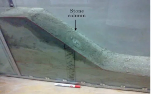
In this model, a stone column with a diameter of 4 cm is installed in the upslope (at x=r = 0:75) (Figure 12). Specications of the stone column are shown in Table 2. In order to install the stone column in the slope, rst, a tube (Figure 12) covered in oil is placed in the upslope. Next, the tube is lled with compacted stone column granules. Following this stage, the tube is gradually pulled out of the slope. Similar to Model 1, soil is saturated by precipitation. After one hour and forty minutes, two minor cracks and one major crack emerge in the slope surface (Figure 13). A larger
Table 1. Values of FS resulting from the 3D FD method (Model 1).
Dry slope Saturated slope Factor of safety 1.08 0.89
Figure 12. Slope reinforced with an upstream stone column (at x=r = 0:75).
Figure 13. The position of the stone column and cracks.
crack emerges in the middle of the slope at x=r = 0:5. The slope experiences failure after one hour and fty-ve minutes. Figure 14 shows the slope section, the position of the stone column, and three cracks. Crack 2, positioned at x=r = 0:5, is larger than Cracks 1 and 3 in terms of width.
Moreover, positions (x=r) of Cracks 1 and 3 are also measured to be 0.13 and 0.67, respectively. 3.5. Analysis of Model 2 using 3D FD method Value of Factor of Safety (FS = 0.95) obtained using the 3D FD method in the stability analysis of Model 2 is shown in Table 3.
Table 3 conrms experimental results. As seen in this table, while the stone column is installed in the upslope (x=r = 0:75), values of factor of safety are ob-tained to be less than 1, reecting the instability of the slope. In experimental tests, the reinforced sand slope (at x=r = 0:75) also yielded failure and experienced instability following the precipitation phase.
3.6. Model 3: Slope reinforced with downstream stone column
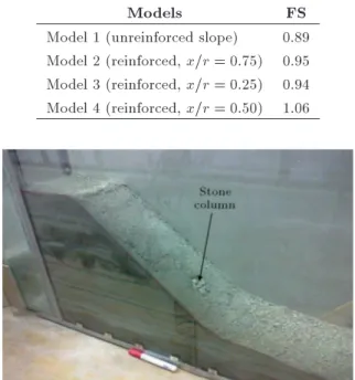
In this model, a stone column with a diameter of 4 cm is situated in the downstream of slope (in position of x=r = 0:25) (Figure 15). After placing the stone col-umn in the downstream, the slope is saturated through precipitation. One hour and twenty minutes later, a V-shaped crack emerges in the slope (Figure 16).
Figure 14. The slope section, the position of the upstream stone column, and three cracks.
Table 2. Specications of the stone column and sand.
Stone column Lower sand Upper sand
Unit weight (kN/m3) 17 18 20
Cohesion (kN/m2) 0:0 0:0 0:0
Friction ( _') 45 45 47
Elastic modulus (MPa) 100 30 30
Table 3. Factor of safety in a saturated condition for all models obtained using 3D FDM.
Models FS
Model 1 (unreinforced slope) 0.89 Model 2 (reinforced, x=r = 0:75) 0.95 Model 3 (reinforced, x=r = 0:25) 0.94 Model 4 (reinforced, x=r = 0:50) 1.06
Figure 15. Slope reinforced with a downstream stone column (at x=r = 0:25).
situated on x=r = 0:5. Figure 17 shows the section of the stone column (before deformation) and the crack in the slope.
3.7. Analysis of model 3 using the 3 FD methods
Values of Factor of Safety (FS = 0.94) obtained using the 3D FD method after performing the stability
Figure 16. V-shaped crack in the slope at x=r = 0:5
analysis of Model 3 are shown in Table 3.
Table 3 conrms experimental results. As seen in this table, when the stone column is located in the downstream of slope (at the position of x=r = 0:25), the obtained factor of safety is less than 1, which reects instability of the slope. In experimental tests, the reinforced sand slope (at x=r = 0:25) also experienced failure and instability following saturation.
3.8. Model 4: Slope reinforced with intermediary stone column
In this model, the stone column was placed in the slope middle (Figure 18). No crack or failure occurred on the slope after two and a half hours of precipitation. Therefore, the slope managed to maintain its stability (Figure 19).
Figure 17. The section of the stone column (before deformation) and the crack in the slope.
Figure 18. The stone column placed in the middle of the slope.
Figure 19. No crack and failure after 2:30 hours of precipitation when stone column is placed at x=r = 0:5.
3.9. Analysis of Model 4 using the 3D FD method
Factor of Safety value (FS = 1:06) acquired by the 3D FD method in a saturated condition after performing the stability analysis of Model 4 is shown in Table 3.
Table 3 conrms experimental results. As ob-served in this table, the value obtained for FS is larger than 1, specifying that the slope is stable. Experimental results also conrm that the slope can
preserve its stability after two and a half hours of precipitation.
4. Eect of length of stone column
In this part, dierent lengths of stone column were analyzed. The stone columns were installed in the upslope, downslope, and intermediate with dierent lengths as follows: length of intermediate stone column = 40 cm and 50 cm, length of upslope stone column = 50 cm and 60 cm, and length of downslope stone column = 30 cm and 40 cm. Tables 4{6 show FS, maximum X- and Y -displacement and maximum shear strain increment for dierent lengths of stone column into intermediate, upslope, and downslope.
Tables 4{6 show that an increase in the length of the stone column has no signicant eect on the reduc-tion of displacement because slip surface is shallow. 5. Slope angles
In addition, two other slope angles, 30 and 60 degrees, have been investigated. For a slope angle of 30 degrees, the unreinforced slope is stable in both dry and saturated states. Table 7 shows FS, maximum X- and Y -displacement, and maximum shear strain increment for a slope angle of 30 degrees. Table 8 shows maximum X- and Y -displacement and maximum shear strain increment for a slope angle of 60 degrees.
Dierent values (30 and 60 degrees) were assumed for slope angle. Tables 7 and 8 show FS, the maximum X- and Z-displacement for the slope angles of 30 and 60 degrees. As the slope angle increases, maximum X-and Z-displacement increases.
6. Discussion
Stabilization of earth slopes using stone columns can be introduced as one of the eective and practical means of stabilization. However, it is important to
Table 4. Eect of dierent lengths for an intermediate stone column. Length of
intermediate stone column
FS
Maximum X-displacement
(mm)
Maximum Z-displacement
(mm)
Maximum shear strain increment
40 cm (dry) 1.17 1:7 10 2 6:9 10 2 9:7 10 4
40 cm (sat) 1.16 1:7 10 2 6:1 10 2 9:2 10 4
50 cm (dry) 1.16 1:9 10 2 1:0 10 1 1:4 10 3
50 cm (sat) 1.14 2:0 10 2 8:2 10 2 1:2 10 3
Table 5. Eect of dierent lengths for upslope stone column Length of
upslop stone column
FS
Maximum X-displacement
(mm)
Maximum Z-displacement
(mm)
Maximum shear strain increment
50 cm (dry) 1.22 9:6 10 3 6:5 10 2 2:0 10 3
50 cm (sat) 0.98 0.30 0.41 2:8 10 2
60 cm (dry) 1.25 7:9 10 3 9:5 10 2 2:9 10 3
60 cm (sat) 0.97 0.14 0.18 1:1 10 2
Table 6. Eect of dierent lengths for upslope stone column. Length of
downslope stone column
FS
Maximum X-displacement
(mm)
Maximum Z-displacement
(mm)
Maximum shear strain increment
30 cm (dry) 1.14 1:4 10 2 6:3 10 2 6:9 10 4
30 cm (sat) 0.94 0.14 0.20 3:8 10 3
40 cm (dry) 1.11 1:9 10 2 9:9 10 2 1:2 10 3
40 cm (sat) 0.97 0.12 0.20 4:3 10 3
Table 7. Eect of a slope angle of 30 degrees on dierent locations of stone columns in a saturated state. Slope angle
of 30 degrees FS
Maximum X-displacement
(mm)
Maximum Z-displacement
(mm)
Maximum shear strain increment Model 1 (unreinforced slope) 1.31 8:3 10 3 3:4 10 2 1:0 10 3 Model 2 (reinforced slope, x=r = 0:75) 1.29 8:8 10 3 3:2 10 2 2:6 10 4 Model 3 (reinforced slope, x=r = 0:25) 1.25 9:6 10 3 3:5 10 2 6:9 10 4 Model 4 (reinforced slope, x=r = 0:50) 1.35 7:7 10 3 3:1 10 2 4:2 10 4 Table 8. Eect of slope angle of 60 degrees on dierent locations of stone columns in a saturated state.
Slope angle of
60 degrees FS
Maximum X-displacement
(mm)
Maximum Z-displacement
(mm)
Maximum shear strain increment
Model 1 (unreinforced slope) 0.83 6.9 4.4 1:1 10 2
Model 2 (reinforced slope, x=r = 0:75) 0.97 0.34 0.42 3:2 10 2 Model 3 (reinforced slope, x=r = 0:25) 0.94 0.27 0.40 1:3 10 2 Model 4 (reinforced slope, x=r = 0:50) 1.00 0.10 0.14 5:7 10 3
choose the best place for the stone column to attain the highest FS and guarantee the stability of slopes. In experimental tests, a sand slope (Model 1) with an angle of 45 degrees and two layers of sand with dierent unit weights were modeled. Moreover, the unit weight
of the lower layer was less than that of the upper layer. The slope is saturated through precipitation. After one hour and twenty minutes, a deep crack emerged in the slope middle, indicating that the slope loses its stability under precipitation. Pore water pressure
Figure 20. Variation of the piezometric water level with time for piezometer # 1.
on earth slopes was measured with piezometric panel. A piezometric panel is composed of 14 piezometer pipes and is used to measure pore water pressure on dierent parts of the slope. The slope was compacted and built in the dry state. Therefore, the initial pore pressure was zero. The slope was compacted and built in the dry state to fail after saturation. If the slope is compacted and built with optimal moisture, it will not fail after saturation. Following the construction of the earth slope, articial rain was induced and pore water pressure increased gradually. Variations of pore water pressure were measured using the piezometers. Figure 20 shows an increase in the piezometric water level over time (for piezometer #1). In fact, piezometric water level increases until the soil is saturated and piezometric water level reaches its peak. It is worth mentioning that, in all models, soil failure occurred following saturation and no crack or failure was observed before saturation. The 3D FD method also revealed the instability of the slope. Model 1 is tested without a stone column; however, the crack in the middle of the slope shows that the middle of the slope is the best place to install the stone column.
Model 2 shows a stone column installed at x=r = 0:75 (upslope). This model is also modeled similar to Model 1 and is exposed to precipitation, too. After one hour and forty minutes, a relatively deep crack emerged at x=r = 0:5. After a while, two minor cracks also emerged at x=r = 0:13 and x=r = 0:67. The presence of the relatively deep crack at x=r = 0:5 revealed that the slope lost its stability in spite of the stone column used to reinforce it. A 3D FD method also conrmed instability of the slope in this model. The presence of the relatively deep crack in the middle of the slope in Model 2 indicated that the highest shear strain was achieved in the slope middle. Depth of cracks in Model 2 is less than that in Model 1, which results from the slope reinforced with upslope stone columns.
The two minor cracks that emerged in Model 2 after the emergence of the intermediary crack show that the middle of the slope is more critical than such places as x=r = 0:13 and x=r = 0:67.
In Model 3, the stone column is positioned at x=r = 0:25 (slope downstream) and is modeled similar to Models 1 and 2. It is subjected to precipitation, too. After one hour and twenty minutes, a relatively deep V-shaped crack was seen in the middle of the slope. The emergence of the crack reects the instability of the slope reinforced by a downstream stone column. 3D FD method also conrmed instability of the slope in this model. The 3D FD method results indicate that the maximum displacement occurred on top of stone column, whose cracks in the experimental test were conrmed.
After all, results of tests performed on Models 1, 2, and 3 prove the instability of the slope. Models 2 and 3 indicate that it is of great importance to choose an optimal location for stone column installation, because if the stone column is not placed in an optimal location, the stability of the reinforced slope will not be guaranteed (Models 2 and 3).
In all experimental models, failure followed satu-ration and none of the models failed during satusatu-ration. The pore water pressure was assumed to be equal to failure time slope pore water pressure in the relation for safety factor calculation. Models 1, 2, and 3 were saturated in the experimental tests through articial rainfall and failed following saturation. At the be-ginning of the experiment, the piezometric water level was zero. This value increased gradually as a result of precipitation until the soil was saturated. In the saturated state, the piezometric water level in the slope was equal to the soil column height at each point. In other words, when the slope was saturated, the piezometric water level remained unchanged and no increase was observed at the piezometric level, and the rest of water was drained by sand.
In Model 4, the stone column is placed at x=r = 0:5 and the slope is subjected to precipitation and modeling similar to Models 1, 2, and 3. The slope was under precipitation for two and a half hours, yet remained stable without any crack. The ndings indicate that the weakest section of the slope was used for reinforcement, because unlike the previous model, it showed no signs of fracture, even after two and a half hours of precipitation. The testers revealed that if the slope is subjected to more than two and a half hours of precipitation, it will still preserve its stability. Therefore, the most critical place is located in the slope middle, which can be overcome by reinforcing the slope. The 3D FD method also conrmed the stability of Model 4. The factors of safety obtained by the three-dimensional nite dierence method for all models are presented in Table 3.
The maximum displacement and shear strain that occurred in all models are presented in Table 9. The results indicate that when the stone column is installed in downstream, the slope will undergo fewer
displace-Table 9. Displacement in a saturated condition for all models obtained using 3D FDM. Models
Maximum X-displacement
(mm)
Maximum Z-displacement
(mm)
Maximum displacement
(mm)
Maximum shear strain
Model 1 (unreinforced slope) 1.29 1.15 1.36 3:6 10 2
Model 2 (reinforced, x=r = 0:75) 0.97 1.26 1.51 3:4 10 2
Model 3 (reinforced, x/r=0.25) 0.14 0.22 0.24 3:8 10 3
Model 4 (reinforced, x=r = 0:50) 3:6 10 2 4:5 10 2 4:8 10 2 8:7 10 4
Table 10. Converting any experimental model into a real with scale ratio S. Time Length Area Force Mass
Real T L A F M
Experimental model pST SL S2A S2F S3M
ments. When the stone column is installed in the upslope, the driving force increases and when the stone column is installed in the downstream, the resisting force increases. However, the dierence between results of Models 2 and 3 is insignicant; they are both unstable. If the model developed in the experimental test fails following saturation, it is concluded that the FS is less than 1. However, even if it does not fail after saturation, it is deduced that the factor of safety is more than 1. The 3D FD method was used to conrm experimental results. The conrmation was carried out by determining the minimum safety factor. That is to say, the 3D FD method calculates the minimum FS, and the obtained values complied with experimental results. In other words, when the experimental model did not lead to failure, safety factor values gained by the 3D FD method were higher than 1; when the experimental model failed, the values of safety factor obtained by the aforementioned method were smaller than 1. However, the forms of the slip surfaces of the three models were almost similar; in addition, the values of factor of safety and the stability/instability of slopes were in agreement.
The numerical models proposed by Wei and Cheng [22], Hajiazizi and Mazaheri [23], Cai and Ugai [8], and Won et al. [10] also introduced the center of the slope as the best place for attaining the highest safety factor. However, other researchers have conducted numerical and analytical studies that suggest other places for pile installation.
To clarify important parameters such as slope angle and length of stone column, a set of 3D nite dierence analyses was carried out. The 3D nite dif-ference method was used for numerical modeling with rectangular mesh. Global and local mesh renements were dened to certify a good quality of the mesh. After conducting sensitive analysis, the total number of meshes was 2548. For the reinforced slope, the number of meshes was 3552, in which stone columns
have 896 meshes. The elements used in this analysis were rectangular. For each number of elements, the most accurate mesh was also searched, i.e., rening the mesh in the area of interest (slope and column) and using a coarse mesh in the far eld. A 3D model of the slope and the column would take a lot of time. 7. Limitations
Scale eects can be applied to enlarge the experimental outcomes to the eld situation using Table 10, in which S is the scaling parameter [1]. Therefore, by using Table 10, we may convert any experimental model into a real one. It should be noted that soil strength char-acteristics, such as angle of internal friction, soil unit weight, and cohesion, stand xed in both real and ex-perimental models after scaling. Hajiani Boushehrian et al. [24] studied a small-scale test box for modeling the behavior and ballast performance under eld condi-tions in the presence of the reinforcement. It is known that because of the scale eects and the nature of soils, especially granular soils, soils may not play the same role in the experimental models as in the prototype [25]. These dierences occur due to the dierences in stress level between the eld tests and the model tests [26]. Nevertheless, because of variations in the stress level, scale eects will occur in earth gravity (1-g) modeling. Therefore, applying 1-g models can be useful in predict-ing only general trends of the behavior of a particular prototype [25]. Therefore, it is suggested performing further investigations using full-scale tests or centrifu-gal model tests to ascertain the obtained results. 8. Conclusion
Stabilization of earth slopes using stone columns can be introduced as one of the eective methods for slope stabilization. Choosing the best place for stone column is an important factor that aects stability or
instabil-ity of the slopes. In order to nd an optimal place to install the stone column, numerous experimental models were created. The model is exposed to articial precipitation. In models where stone columns were not located in the middle of the slope, cracks developed from the center of the slope and the slope yielded failure with the continuation of precipitation. However, in the model that was reinforced with an intermediary stone column, no failure or crack was observed. Of note, the model was subjected to similar modeling and precipitation conditions. The tests, which were per-formed on two-layer sand soil, indicated that the most critical part of sand slope was its center. Therefore, reinforcing the middle of the slope guarantees slope stability. Results of the 3D FD method also conrmed experimental results. It was revealed that when the stone column was placed in the middle of the slope, the value of factor of safety exceeded 1; however, when it was placed elsewhere, the factor of safety was less than 1. Numerous numerical studies by other researchers also introduced the center of the slope as the most critical part of the slope. However, the authors of the article believe that, in granular soils, the highest shear strain was achieved in the middle of the slope. Therefore, any reinforcement must be performed in the middle of the slope to obtain the highest factor of safety.
References
1. Hajiazizi, M., Bavali, M., and Fakhimi, A. \Numerical and experimental study of the optimal location of concrete piles in saturated sandy slope", International Journal of Civil Engineering, 16(10), pp. 1{9 (2017).
2. Poulos, H.G. \Design of reinforcing piles to in-crease slope stability", Canadian Geotechnical Journal, 32(5), pp. 808{818 (1995).
3. Lee, C.Y., Hull, T.S., and Poulos, H.G. \Simplied pile-slope stability analysis", Computers Geotechnics, 17, pp. 1{16 (1995).
4. Hassiotis, S., Chameau, J.L., and Gunaratne, M. \Design method for stabilization of slopes with piles", Journal of Geotechnical and Geoenvironmental Engi-neering, ASCE, 123(4), pp. 314{323 (1997).
5. Ito, T. and Matsui, T. \Methods to estimate lateral force acting on stabilizing piles", Soils and Founda-tions, 15, pp. 43{59 (1975).
6. Ito, T., Matsui, T., and Hong, W.P. \Design method for the stability analysis of the slope with landing pier", Soils and Foundations, 19(4), pp. 43{57 (1979).
7. Ito, T., Matsui, T., and Hong, W.P. \Design method for stabilizing piles against landslide- one row of piles", Soils and Foundations, 21(1), pp. 21{37 (1981).
8. Cai, F. and Ugai, K. \Numerical analysis of the stability of a slope reinforced with piles", Soils and Foundations, 40(1), pp. 73{84 (2000).
9. Ausilio, E., Conte, E., and Dente, G. \Stability analysis of slopes reinforced with piles", Computers and Geotechnics, 28, pp. 591{611 (2001).
10. Won, J., You, K., Jeong, S., and Kim, S. \Coupled eects in stability analysis of pile-slope systems", Computers and Geotechnics, 32, pp. 304{315 (2005).
11. Nian, T.K., Chen, G.Q., Luan, M.T., Yang, Q., and Zheng, D.F. \Limit analysis of the stability of slopes reinforced with piles against landslide in nonhomoge-neous and anisotropic soils", Canadian Geotechnical Journal, 45(8), pp. 1092{1103 (2008).
12. Xinpo, L., Xiangjun, P., Marte, G., and Siming, H. \Optimal location of piles in slope stabilization by limit analysis", Acta Geotechnica, 7, pp. 253{259 (2012).
13. Zhang, G. and Wang, L. \Integrated analysis of a coupled mechanism for the failure processes of pile-reinforced slopes", Acta Geotechnica, 11(4), pp. 941{ 952 (2016).
14. Castro, J. \An analytical solution for the settlement of stone columns beneath rigid footings", Acta Geotech-nica, 11, pp. 309{324 (2016).
15. Nazari Afshar, J. and Ghazavi, M. \A simple analyt-ical method for calculation bearing capacity of stone column", International Journal of Civil Engineering, 12(1), pp. 15{25 (2014).
16. Hajiazizi, M., Kilanehei, P., and Kilanehei, F. \A new method for three dimensional stability analysis of earth slopes", Scientia Iranica, 25(1), pp. 129{139 (2018).
17. Hajiazizi, M., Nasiri, M., and Mazaheri, A.R. \The eect of xed piles tip on stabilization of earth slopes", Scientia Iranica, 25(5), pp. 2550{2560 (2018).
18. Hajiazizi, M., Mazaheri, A.R., and Orense, R.P. \Ana-lytical approach to evaluate stability of pile-stabilized slope", Scientia Iranica, 25(5), pp. 2525{2536 (2018).
19. Ghanbari, E. and Hamidi, A. \Stability analysis of dry sandy slopes adjacent to dynamic compaction process", Scientia Iranica, 24(1), pp. 82{95 (2017).
20. Hajiazizi, M. and Tavana H. \Determining three-dimensional non-spherical critical slip surface in earth slopes using an optimization method", Engineering Geology, 153, pp. 114{124 (2013).
21. Ambily, A.P. and Gandhi, S.R. \Behavior of stone columns based on experimental and FEM analysis", J Geotech Geoenviron Eng., 133(4), pp. 405{415 (2007).
22. Wei, W.B. and Cheng, Y.M. \Strength reduction analysis for slope reinforced with one row of piles", Computers and Geotechnics, 36, pp. 1176{1185 (2009).
23. Hajiazizi, M. and Mazaheri A.R. \Use of line segments slip surface for optimized design of piles in stabilization of the earth slopes", International Journal of Civil Engineering, 13(1), pp. 14{27 (2015).
24. Hajiani Boushehrian, A., Vafamand, A., and Kohan, S. \Investigating the experimental behavior of the reinforcements eect on the railway traverse under the dynamic load", Scientia Iranica, 24(5), pp. 2253{2261 (2017).
25. El-Sawwaf, M.A. \Strip footing behavior on pile and sheet pile-stabilized sand slope", Journal of Geotechni-cal and Geoenvironmental Engineering, 131, pp. 705{ 715 (2005).
26. Vesic, A.S. \Analysis of ultimate loads of shallow foun-dations", Journal of Soil Mechanics and Foundations Division, 99(1), pp. 45{73 (1973).
Biographies
Mohammad Hajiazizi is an Associate Professor of Geotechnical Engineering at Razi University, Kerman-shah, Iran. He received his PhD degree in Geotechnical Engineering from Shiraz University in Iran and his MSc degree in the same eld from Tarbiat Modares Uni-versity, Tehran, Iran. His current and main research interests include soil improvement, slope stability, tun-neling, and meshless methods.
Esmail Nemati graduated with an MSc degree in Geotechnical Engineering from Razi University, Ker-manshah, Iran. He received his BS degree from Jahad-e DanJahad-eshgahi. His currJahad-ent rJahad-esJahad-earch intJahad-erJahad-ests includJahad-e slope stability and numerical modeling of the soil structures.
Masoud Nasiri is a PhD Student in Geotechnical En-gineering from Razi University, Kermanshah, Iran. He received his MSc degree in Geotechnical Engineering from Razi University, Kermanshah, Iran.
Moslem Bavali graduated with an MSc degree in Geotechnical Engineering from Razi University, Ker-manshah, Iran. He received his BS degree from Jahad-e Daneshgahi, Kermanshah branch. His current research interests include slope stability and numerical modeling of the soil structures.
Mohammad Sharipour is an Assistant Professor of Civil Engineering at Razi University, Kermanshah, Iran. He received his PhD degree in Civil Engineering from Central Nanets in France and his MSc degree in Hydraulic Structures from the Amirkabir University of Technology. His current and main research interest is bender element test.