Comparing Euclidean and River Distance Metrics in the Bayesian Maximum Entropy (BME) Estimation of E. coli Concentrations in Connecticut Rivers
John Cordes
Advisor: Dr. Marc Serre
Committee Reader: Dr. Jill Stewart
Committee Reader: Mr. David Holcomb, PhD Candidate
Abstract
Due to budget and personnel constraints, Connecticut is unable to collect data for E. coli concentration for every site every day. The Bayesian maximum entropy (BME) framework for geostatistical estimation integrates general knowledge about the space/time random field and site-specific knowledge. We developed a method to optimize the global offset function, comparing Euclidean and river distance metrics. By shrinking the kernel, we saw that as the variance decreases for the river distance approach, the spatial range holds steady. For covariance modeling, we found that river distance could estimate concentrations at a longer spatial range than could be accounted for by the tortuosity. We found areas of high concentration in the north central portion of the state and low concentrations in the east. We calculated the number of impaired river miles and we estimate that about 34% of river reaches under study had a greater than 50% chance of being impaired.
Introduction
The fecal-oral route is a common mode of transmission for pathogens and in 2011-2012, there were 90 outbreaks of recreational water-associated diseases in the US resulting in at least 1,788 cases (Hlavsa et al., 2015). Common fecal-oral diseases include Hepatitis A, Norovirus gastroenteritis, and Salmonellosis (Zuckerman et al. 1996; CDC, 2015; Gantoi et al., 2009). People become infected by drinking contaminated water or by submersion and entrance through the mucous membranes (CDC, 2016). The latter mode of transmission is especially important in recreational swimming and boating waters.
Several different methods exist for measuring water fecal contamination including measuring for fecal coliforms, Escherichia coli (E. coli), and Enterococci concentrations (EPA, 2000). These bacteria, while oftentimes not pathogenic themselves, are important indicators to identify other pathogens in water (Money et al., 2009(a)). The US Environmental Protection Agency (EPA) recommends measuring for E. coli concentration for fresh water fecal
contamination (EPA, 2012). By measuring E. coli, we can get a general sense about how polluted the water is from human or animal waste. The EPA sets standards for E. coli concentration in recreational waters such as rivers and lakes through the Clean Water Act (CWA) of 1986 and the Beaches Environmental Assessment and Coastal Waters (BEACH) Act of 2000 (EPA, 2012). These standards are updated periodically and the most recent revisions came in 2012. The current standards for E. coli concentration (colony forming units per 100mL) in recreational fresh waters are a 30-day geometric mean of 126 cfu/100mL or a 30-day standard threshold value of 410 cfu/100mL. The standard threshold value should not be exceeded by more than 10% of samples taken during the time period (EPA, 2012). The EPA uses 30-day metrics because water quality is highly variable and susceptible to weather events (EPA, 2012).
While the EPA provides the above recommendations, water quality regulations are set by individual states. The Connecticut Department of Public Health (CTDPH) sets standards for recreational swimming closures based on E. coli concentrations similar to the EPA, but not exactly. Connecticut uses the 30-day geometric mean of 126 cfu/100mL or less, but it also has a daily sample threshold value of 235 cfu/100mL. If the single day value is exceeded, the
The state of Connecticut performs surface water monitoring of key indicator bacteria, including E. coli, to test for contamination that can lead to illness. However, due to budget and personnel constraints, it is impossible to collect data for all river miles every day, let alone each site every day. The state could use geostatistical estimation techniques to determine the
approximate levels of E. coli for unmeasured river miles in order to identify impaired waterways and protect public health. Traditional geostatistical estimation techniques consider only
knowledge of autocorrelation of the phenomenon in space and use Euclidean distance metrics. Space-only methods ignore the information garnered from other values near in time. Bayesian maximum entropy (BME) of modern space/time geostatistics provides the opportunity to incorporate knowledge of autocorrelation of the phenomenon in time as well as space (Jat and Serre, 2016). A further advantage of BME techniques is the ability to create estimations along the river network in addition to Euclidean distances (Money et al., 2009(b)). Several studies have used river network distance instead of Euclidean distance measures to successfully estimate E. coli (Money et al., 2009(a)) as well as other water quality measures (Jat and Serre, 2016; Money et al., 2009(b); Money et al., 2011). However, no study to our knowledge has examined
optimization of the global offset function in terms of Euclidean and river distance covariance models or the effects of river tortuosity in the estimation of E. coli. Furthermore, we explore the effects of these different metrics on estimation mapping and impairment designation. Optimal selection of these BME parameters is essential to producing an appropriate, accurate estimation at any given space/time location. Different parameters can produce drastically different
estimation maps and it is important to understand these differences to produce the best possible estimation.
Research Questions
How do we select an optimal global offset function using both Euclidean and river distance metrics? Do river distances capture more spatial autocorrelation in E. coli concentration distribution versus Euclidean distances? What percentage of river miles are impaired in
Connecticut and what are the effects of Euclidean versus river distance approaches on impairment designation?
Materials and Methods
Study Area and E. coli Concentration Data
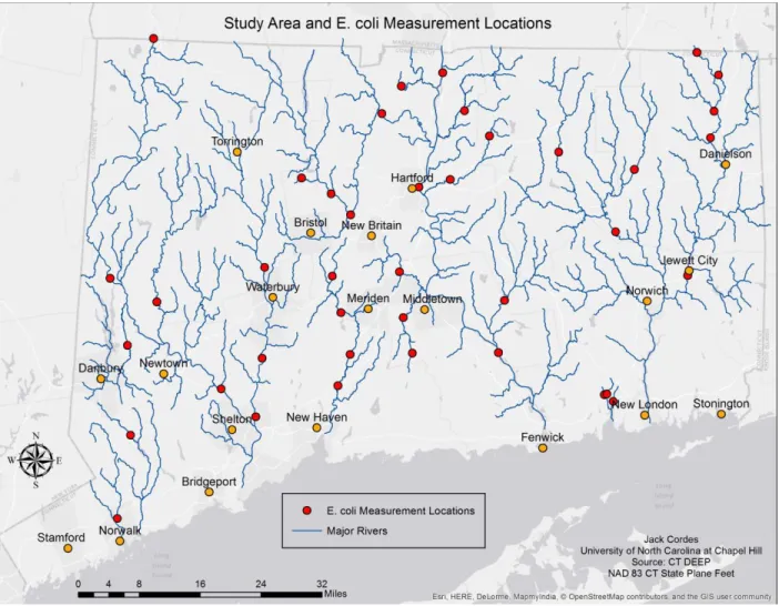
The area under study includes the entire state of Connecticut. Connecticut contains three primary watersheds, all of which empty into the Long Island Sound. They are, west to east, the Housatonic River, the Connecticut River, and the Thames River.
Figure 1. Study area
Measurements in the dataset from the NWIS come in four different forms. The first form is a true measure that is within the bounds of detection. The second form comes with an “E” in front indicating an estimated value. The third form has a less than sign (“<”) preceding the value, which means the measurement was below the detection limit. The fourth form has a greater than sign (“>”) preceding the value, which means the measurement was above the maximum
detection limit. The estimate and above detection soft data were hardened by removing the “E” or the “>” to set estimated values as true values. Measurements below the detection limit were divided by 2 and accepted as hard data points. The entire study period included 2,468 data points. Of these, 3 measurements were estimates, 45 were above the detection limit, and 6 were below the detection limit. These measurements are taken at irregular intervals at various stations across the state resulting in asynchronized sampling data. For the remainder of the analysis, we will use the individual data points with no aggregation despite regulations based on 30-day intervals. The reason for this is because no stations consistently have the necessary
Furthermore, stations that are consistently above this threshold over the study period would be areas of concern for chronic fecal contamination.
River Network Construction
A polyline shapefile of major rivers was obtained from the Connecticut Department of Energy and Environmental Protection (DEEP) (DEEP, 2016). We selected only the watersheds for which E. coli measurements were taken during the study period. The rivers included from west to east were the Norwalk, Saugatuck, Housatonic, Quinnipiac, Connecticut, Niantic, and Thames. We converted the line file to a series of points describing the network and built the BMEGUI river network file by selecting each river reach and copying the latitude and longitude locations of the points to a new file. This final river network file contains a set of points
representing each river reach separated by NaN values with an outlet point designated at the end. Since BMEGUI cannot handle multiple, independent river networks, we artificially combined all the river networks in Connecticut into a single network with a single outlet by connecting the outlets of each individual river network together.
Bayesian Maximum Entropy (BME) Estimation Framework
The method of analysis in this study is rooted in the BME framework commonly used in modern geostatistical analyses. We use the framework to estimate E. coli concentrations at positions in space and time for which there are no measured values. The estimations are made in the context of a space/time random field (S/TRF) denoted as 𝑋(𝑝), where 𝑝 = (𝑠, 𝑡) represents a particular position in space/time. The random variable vector 𝒙(𝑝) represents the complete set of possible values for 𝑋(𝑝) at every position. Therefore the S/TRF, 𝒙𝑚𝑎𝑝, consists of a vector of random variable realizations of 𝑋(𝑝) (Akita et al., 2007).
𝒙𝑚𝑎𝑝 = (𝑥1, … , 𝑥𝑣), 𝒑𝑚𝑎𝑝 = (𝑝1, … , 𝑝𝑣)[1]
Where 𝒙𝑚𝑎𝑝 is a collection of all possible realizations and 𝒑𝑚𝑎𝑝 represents all possible locations in space/time. From here, we can develop a probability density function (PDF)
(Equation 2) for the S/TRF by assigning probabilities to each corresponding realization (Akita et al., 2007).
𝑓(𝒙𝑚𝑎𝑝, 𝒑𝑚𝑎𝑝)𝑑𝑥𝑚𝑎𝑝 [2]
Using this BME framework, we produce a stochastic estimation of E. coli concentration at every space/time position in Connecticut over the study period 2006 to 2016. We start by developing general knowledge constraints G. The general knowledge consists of global features we can extract such as the mean trend through all the data or the covariance model that
the E. coli concentration at every location 𝑝 in Connecticut for the study period 2006 to 2016. Finally, we can produce maps and time-series graphs of the concentrations to determine areas of high and low concentration. We refer the reader to Christakos et al. (2002) for further
information on the BME framework and a detailed outline of its numerical implementation.
Euclidean Approach versus River Approach
A fundamental part of this study is the determination of the differences between Euclidean and river network approaches in concentration estimation. Euclidean distance approaches use straight line, “as the crow flies” distances. It assumes no barriers and that
features that are closer to one another in space are more similar than those farther away (positive autocorrelation). River distance approaches are constricted to a specified river network.
Estimation parameters use the river network as a barrier and features are only considered similar if they fall near one another along the network.
In terms of estimation, parallel river reaches can show the stark contrast between the different techniques. Two river reaches that run near to one another but are not part of the same watershed will influence one another and produce similar estimations using Euclidean distance, while the river distance approach would produce different estimates since they are separated by the network. In this example, the river network approach may produce a better estimate,
particularly if the phenomenon is constricted to the river network (e.g. salmon mercury concentrations); however, if the phenomenon exhibits a Euclidean distribution (e.g. a point source isotropic diffusion of pollution between two parallel reaches) the two estimation
techniques may be similar. The difference between Euclidean and river distances most directly affects the spatial range parameter. River distance approaches tend to have longer spatial ranges, which would appear to be an advantage, however we must consider the effects of tortuosity. Is the river distance spatial range actually creating better predictions over longer distances or are the twists and turns adding distance in the river approach and simply inflating the spatial range metric without improving the estimation? To determine the tortuosity of rivers in Connecticut, we measured both the Euclidean and river distance of every river reach in the dataset. We calculated average tortuosity by dividing the sum of the river distances by the sum of the
Euclidean distances. To evaluate the effects of tortuosity on the estimation model, we compared three different scenarios for the spatial range in the covariance model using river distances: equal to the Euclidean model, equal to the Euclidean model multiplied by the tortuosity, and equal to the appropriate range based on the river distance model. In theory, the river distance model using the Euclidean range multiplied by the tortuosity should yield the same range as the appropriate spatial range and produce the closest estimation maps to the purely Euclidean model. If the appropriate spatial range for the river distance model is longer than the Euclidean multiplied by the tortuosity, then it would suggest that the river distance model is performing better in terms of defining autocorrelation in E. coli concentration.
Optimal Global Offset Function
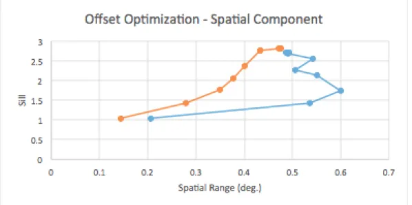
that aid in defining an appropriate covariance model (Akita et al., 2007; Jat and Serre, 2016). However, the size of this kernel is subject to modeler’s choice. An uninformed global offset function has a large space/time kernel and calculates a global average through the data. When removed from the data, an uninformed global offset will return the exact variation that was originally present in the data because the residuals are all calculated with respect to the same value. In contrast, an informed global offset function has a small space/time kernel and closely follows the variation in the data. Yet, while it reduces variability in the data, we also lose all the information provided by autocorrelation. To characterize this trade-off and determine the appropriate offset function, we tested different offsets and evaluated the variance against the spatial and temporal ranges in the subsequent covariance model using the automatic modeler in BMEGUI. Furthermore, we evaluated the differences using Euclidean versus river distance metrics. Beginning with the uninformed global offset incorporating all data in space and time (i.e. calculating a global average), we proceeded to shrink the space/time kernel in a step-wise fashion until we reached an informed offset that compared points against themselves. We plotted the spatial and temporal ranges against the variance at each step and optimized the model by selecting the kernel that produced simultaneously a low variance and high range.
BMEGUI Tool
The primary tool of analysis is the software BMEGUI 3.0.1 (Jat and Serre, 2014). BMEGUI is a python 2.5-based software that incorporates the BMElib package as well as
MATLAB Compiler Runtime (MCR). The software includes a progression of 7 screens. The first screen is workspace, data, and river network selection. BMEGUI is capable of reading .txt and .csv formats. The second screen allows the user to select particular variable fields including data location and measurement values. It also includes an option for datatype, in which the user can incorporate soft data values. The third screen is an exploratory analysis of the histogram, which provides the four statistical moments and the option to log-transform the data. The fourth screen is a continuation of the exploratory analysis. It provides time-series graphs for each station and maps for each time stamp. In this stage, the user may also choose whether to aggregate the data by a specified time interval, in which case BMEGUI will average all values for a particular station within the aggregation time period to a single value. The fifth screen provides the option to set and remove the global offset function from the data. The user can choose to set smoothing ranges both spatially and temporally. The sixth screen is covariance modeling. BMEGUI
Comparison with Space-Only Euclidean Estimation
In the absence of temporal autocorrelation knowledge, BME estimation can be reduced to space-only estimation (Christakos and Li, 1998). In the BME framework, this means that 𝑡 −
𝑡′= 0 and the temporal component of the covariance model becomes 1, leaving just the spatial component. To understand the benefits of incorporating temporal information, we conducted space-only estimation at a single point in time using Euclidean measures and compared the estimation map to the map created with the space/time model.
River Reach Impairment Status
In order to understand whether river reaches may be in violation of the Connecticut state water quality standards and in the interest of protecting public health, it is important to know which river reaches may be classified as unsuitable for recreation (impaired). Based on the Connecticut single day sample threshold, the more conservative regulation at 235 cfu/100mL, we dichotomized the Euclidean distance and river distance estimation maps at that level. Then we associate a probability with this threshold. River reaches above the threshold have a greater than 50% chance of being impaired, while river reaches below the threshold have a less than 50% chance of being impaired. Using this dichotomy, we calculate the number of river miles classified with a high probability of being impaired using both Euclidean and river distance measures.
Results
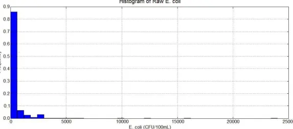
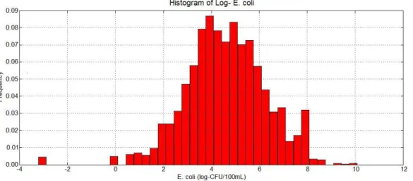
In an exploratory analysis of the data, the raw histogram of individually measured values exhibits a highly positive skew (Figure 2). To correct for this skew, we applied a natural log transformation of the data, which provides a more normal distribution and improves the skewness measure (Figure 3).
Figure 3. Log-transformed E. coli concentration data
The mean average value of the raw data was 361 cfu/100mL, well above the single day standard of 235 cfu/100mL. Of 2,468 measurements, 744 were above this standard and
exceeding the value for safe recreation, representing 30% of all measurements. Initial analysis of the log-transformed moments yields a mean of 4.60 log-cfu/100mL, a standard deviation of 1.68 log-cfu/100mL, and a range of [-3, 10]. These values are summarized in Table 1. A raw spatial mean trend indicated areas of high concentration in the central part of Connecticut along the Quinnipiac and Connecticut Rivers (Figure 4). The river network had a tortuosity of 1.31.
Table 1. Statistical moments: raw vs. log-transformed
Moment Raw Data Log Data
Mean 361 4.60
Standard Deviation 1015 1.68
Skewness 13.5 -0.37
Figure 3. Raw Mean Trend
Global Offset Optimization
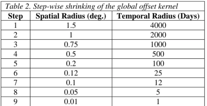
Global offset analysis began with a 1.5 decimal degree and 4,000-day kernel, encompassing the entire dataset. In a step-wise fashion, we dropped the kernel size until it reached 0.01 decimal degrees and 1 day, comparing points only to themselves (Table 2).
Table 2. Step-wise shrinking of the global offset kernel
Step Spatial Radius (deg.) Temporal Radius (Days)
1 1.5 4000
2 1 2000
3 0.75 1000
4 0.5 500
5 0.2 100
6 0.12 25
7 0.1 12
8 0.05 5
9 0.01 1
Euclidean and river distances, Figure 4 shows the trend for the spatial component and Figure 5 shows the trend for the temporal component.
Figure 4. Euclidean: Orange, River: Blue
Figure 5. Euclidean: Orange, River: Blue
Covariance Functions for E. coli Concentrations
The covariance model represents the general relationship in space/time between any two positions in the S/TRF of interest. Experimental covariances are calculated at experimental lags in space only (𝑟 = ||𝑠 − 𝑠′||) and in time only (𝜏 = ||𝑡 − 𝑡′||). Then an additive covariance model is created and may be nested with different behaviors at increasing lags. A general form of the exponential equation is presented in Equation 3.
𝑐𝑥(𝑟, 𝜏) = 𝑐1𝑒−3𝑟 𝑎⁄ 𝑟𝑒−3𝑡 𝑎⁄ 𝑡 [3]
Where 𝑐1is the sill, 𝑟 and 𝑡 are the spatial and temporal lags respectively, and 𝑎𝑟 and 𝑎𝑡 are the spatial and temporal ranges respectively. BMEGUI produces experimental covariance values by selecting pairs of points (𝑝, 𝑝′) for which 𝑟 and 𝑡 are known, 𝑐𝑥(𝑝, 𝑝′) = 𝑐𝑥(𝑟 =
||𝑠 − 𝑠′||, 𝜏 = ||𝑡 − 𝑡′||). Using these experimental values, we can fit a specific covariance model to our E. coli concentration.
For simplicity of comparison, all models presented in this study follow Equation 3 with one component each for space and time. Furthermore, since the only difference between models was the use of Euclidean or river distances, the sill and temporal components are the same for all models. The sill (𝑐1) was equal to 1.7577 and the temporal range (𝑎𝑡) was equal to 350 days (Figure 6). The pure Euclidean covariance model (Figure 7) had a spatial range (𝑎𝑟) of 0.275 decimal degrees. For comparison, we plotted the exact same model with the Euclidean spatial range on the experimental covariances using river distances (Figure 8).
Figure 6. Temporal Covariance
Figure 8. River Distance with Euclidean Spatial Range
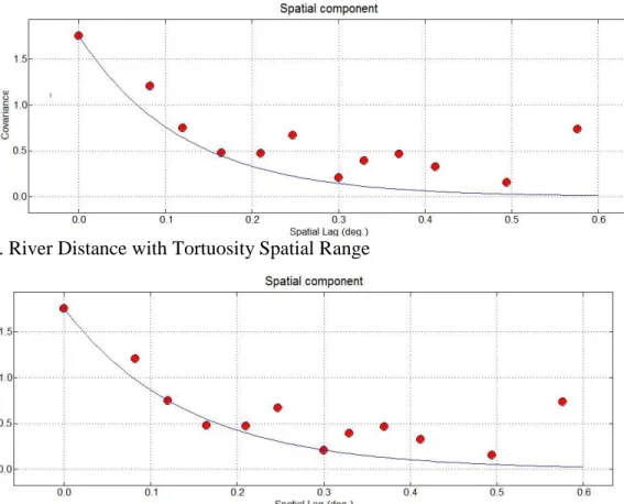
Using the tortuosity calculated for all the river reaches, we created a covariance model based on the theoretical autocorrelation that would be seen assuming that both Euclidean and river distance models are equal. The spatial range for the tortuosity model was 0.36 decimal degrees (Figure 9). Finally, we created a covariance model based on the best fit for the river distance experimental covariances. The spatial range for the river distance model was 0.425 decimal degrees (Figure 10). By dividing the river distance spatial range by the Euclidean spatial range, we obtain an R value of 1.55, which is greater than the tortuosity of 1.31. Furthermore, the spatial range for the river distance model is 18% more than that of the tortuosity.
Figure 9. River Distance with Tortuosity Spatial Range
Estimation Maps
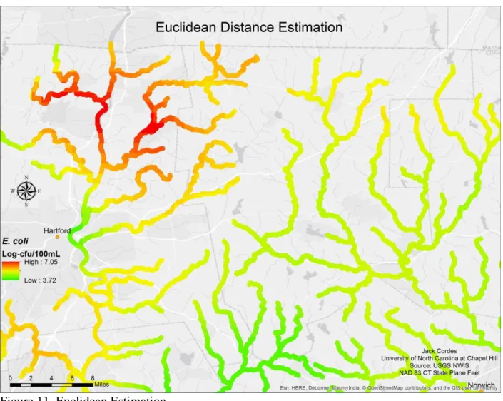
Our exploration date for mapping in this study is August 25, 2009. We selected this date because it had 7 measurements for E. coli concentration, the most of any date in the study period. In addition, for illustration purposes, all maps show an inset of north central Connecticut to highlight the estimation differences between parallel river reaches of two different watersheds, the Connecticut and the Thames. Figure 11 shows the estimation results from the purely Euclidean model using the covariance model depicted in Figure 7.
Figure 11. Euclidean Estimation
This map represents the default estimation technique in most studies. On this particular date, the estimation identifies high E. coli concentrations north of Hartford and low
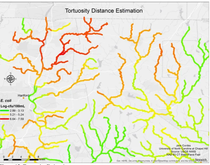
Figure 12. Tortuosity Estimation
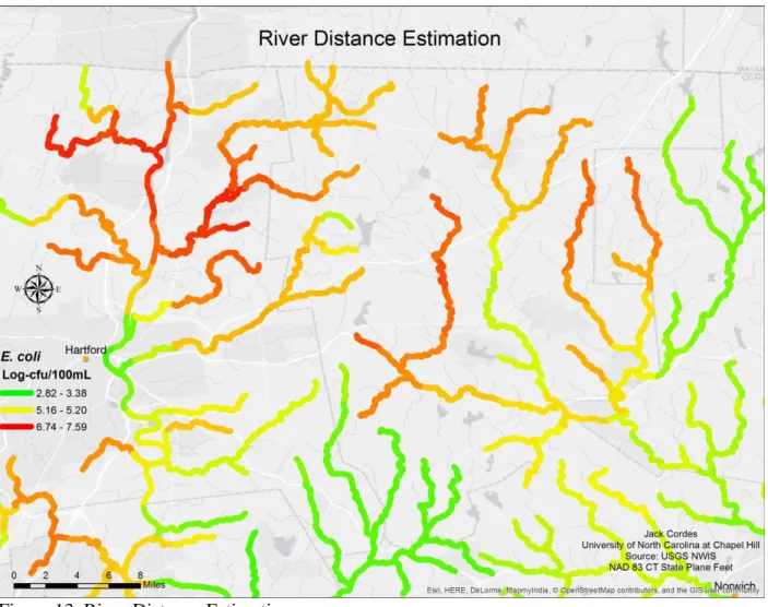
The tortuosity estimation shows major differences from the Euclidean estimation. The river distance estimation shows a more nuanced and intuitive spatial pattern by limiting influences on the concentration in the Thames River watershed from the Connecticut River watershed. River reaches in the center of the figure that are near in space but parts of different watersheds show different concentrations in the river distance estimations; these same reaches show similar concentrations in the Euclidean distance estimation. The low values in the
Connecticut River watershed appear to be influencing values in the Thames River watershed and may be producing artificially low values in the Euclidean distance estimation. Furthermore, we can see within-watershed differences in the Thames River in the eastern part of Figure 12 where parallel river reaches have little influence on one another, but their effects average out at the point where the reaches converge.
Figure 13. River Distance Estimation
Figure 13. Space-only Euclidean Estimation
River Reach Impairment Status
Figure 14. Euclidean Distance Impairment
Discussion
E. coli measurements from the state of Connecticut over the past 10 years show that the average concentration is above the single day standard and almost a third of individual
measurements themselves were above the standard, a sizeable proportion which may be cause for concern. The raw average values for the entire study period indicated high concentrations along the central and southwestern portions of the state including high population areas such as Hartford and Stamford. These areas may be of particular concern for consistently high E. coli concentrations versus the average for Connecticut.
Our global offset function analysis yielded stark differences between using Euclidean and river distance metrics in the spatial domain. The Euclidean distance metric produced the standard curve expected of a decreasing kernel size. A large kernel and uninformed global offset yielded a high sill and high spatial range. The small kernel and informed global offset yielded a low sill and low spatial range. The data points in between the two extremes produced an S-shaped curve that models the trade-off, which had a clear inflection point at a sill of 2.04 cfu/100mL2 and a spatial range of 0.38 decimal degrees. The river distance metric produced a very different curve. As the kernel size decreased, the sill also decreased, but the spatial range stayed relatively constant and even increased until dropping off at the smallest kernel size. This is a novel finding and shows the strength of using a river distance metric. The temporal component of the global offset function showed a linear decrease in both the sill and the temporal range for both
Euclidean and river distance metrics. This pattern indicates that no kernel size is better than any other and that there is an unbiased trade-off between an uninformed and an informed offset function.
The covariance modeling corroborated the strength of using a river distance metric. Using the same global offset function for all covariance models, the river distance model produced a spatial range that was 18% beyond what was predicted by the tortuosity alone. This suggests that the river distance metric is truly capturing more spatial autocorrelation in the data than the Euclidean metric, lending more power to its estimation ability and indicating that E. coli concentrations may be constrained by the river network or influenced by phenomena along the network. The estimation maps for August 25, 2009 revealed major differences for the selected inset area northeast of Hartford. The Euclidean estimation, without the constraints of the river network, mixed concentration information across the Connecticut and Thames River watersheds and appears to have artificially depressed values in the Thames watershed that were parallel to the Connecticut watershed. In particular, the Skungamaug River reach in center of the inset changes from low concentrations in the Euclidean estimation to high concentrations in the river distance estimation. This river reach highlights the importance of using the appropriate method in order to direct surveillance and intervention efforts. Using the Euclidean estimation technique, as is usual, analysts would have missed the high concentrations in the Skungamaug River
because of the protective effect of being close in location to Connecticut River watershed reaches that had low concentrations, despite having no physical influence on one another in the real world.
very smooth trend that does not reveal the nuances in concentration across different river reaches.
The most relevant consideration for regulators is the designation of particular river reaches as impaired (unsuitable for recreation) or unimpaired (suitable for recreation). The method of estimation is crucial when determining potential legal implications and implementing advisories and warnings. Based on the average concentration of E. coli over the study period, no river reaches exceeded the Connecticut single day threshold for recreation. This finding is positive for Connecticut and suggests long-term safety of particular reaches is not a concern. Exploring the difference between Euclidean and river distance metrics on impaired status on a single date, August 25, 2009, we can see the importance of using the best possible model. The river distance metric identified 32% more impaired river miles versus the Euclidean metric. This is a substantial increase and shows how many river reaches may be missed simply with a
Euclidean model. Several river reaches in the Thames watershed, including the Skungamaug River, were identified by the Euclidean metric as unimpaired, but became impaired with the river distance metric. Furthermore, with regard to impaired status, the river distance metric makes more intuitive sense than the Euclidean metric. There are several areas in the Euclidean distance estimation that contain striped river reaches of impaired and unimpaired status, which is highly unlikely. The river distance metric maintains the integrity of river reaches and limits the
influence of parallel river reaches that could lead to striping.
This study has several limitations. The analysis is a rigorous qualitative interpretation instead of a quantitative analysis, which is more typical. We were unable to perform
cross-validation to determine quantitative differences between the Euclidean and river distance models. Instead, we compared the effectiveness of the models by exploring differences in parallel river reaches and the location and number of impaired river miles. A second limitation was the inability to calculate 30-day geometric means for E. coli concentrations as a standard; therefore, we were forced to use the single day threshold. However, considering that the single day
threshold is higher than the 30-day geometric mean, our analyses may be conservative. Lastly, we do not present a formal analysis of the confidence of our estimates in the form of variance values at estimation points. Future work should take these internal variance measures into account.
Moving forward, studies should examine the land use/land cover classes associated with areas of high and low E. coli concentration to determine potential sources of E. coli. This work can identify features in the landscape that occur along the river network and may be influencing the concentrations (e.g. vegetative buffers). Furthermore, future work could depict the
concentration patterns over time by creating animations. These animations can help highlight particular periods of high and low concentrations and would be useful for determining whether there is any seasonality in E. coli concentrations in Connecticut.
Conclusion
and river distance metrics in the selection of an optimal global offset function, the creation of covariance models, the estimation of E. coli concentrations, and the designation of impaired river miles. We found that Euclidean distances in the global offset function followed the typical S-shaped curve with a shrinking kernel. However, river distances produced higher spatial ranges at lower sills, a novel finding. The covariance modeling corroborated the power of the river
distance metric by yielding a spatial range that was 18% longer than that predicted by the
difference due to tortuosity alone. These two findings together suggest that river distance metrics are capturing more spatial autocorrelation in E. coli concentration data and that those E. coli concentrations may be constrained or influenced by the river network. An analysis of the estimation maps showed stark contrasts between Euclidean and river distance metrics. The Euclidean distance estimation experienced information “bleeding” from one watershed to another, whereas the river distance estimation was constrained to the river network and kept parallel river reaches separate. Emblematic of this difference was the Skungamaug River on August 25, 2009, which had low, unimpaired values using Euclidean distance, but high, impaired values using river distance. Average concentrations over the entire study period yielded no impaired river reaches; however, on August 25, 2009, the river distance metric identified 32% more impaired river miles versus the Euclidean distance metric and the river distance estimation limited impaired/unimpaired striping along particular river reaches. Our findings lend support to the use of river distance metrics in the space/time estimation of E. coli concentrations in rivers and we recommend that state agencies pursue river distances as a standard for estimating river reach impairment.
References
US Environmental Protection Agency. “2012 Recreational Water Quality Criteria”. Office of Water. EPA – 820-F-12-061. December 2012.
Akita, Y., Carter, G., & Serre, M. L. (2007). Spatiotemporal nonattainment assessment of surface water tetrachloroethylene in New Jersey. Journal of environmental quality, 36(2), 508-520.
ArcGIS 10.4. ESRI. Redlands, CA.
Centers for Disease Control and Prevention. “Norovirus Illness: Key Facts”. Jan 2015.
Centers for Disease Control and Prevention. “Recreational Water Illnesses”. May 4, 2016. Accessed November 29, 2016.
Christakos, G., Li, X. (1998). Bayesian maximum entropy analysis and mapping: A farewell to kriging estimators?. Mathematical Geology, 30(4).
Christakos, G., P. Bogaert, and M.L. Serre. Temporal GIS: Advanced functions for field-based applications. Springer, New York. 2002.
Connecticut Department of Public Health, Connecticut Department of Energy & Environmental Protection. “State of Connecticut Guidelines for Monitoring Swimming Water and Closure Protocol”. Mar 2016.
Gantois, I.; Ducatelle, R.; Pasmans, F.; Haesebrouck, F; Gast, R.; Humphrey, T.J.; Van Immerseel, F. "Mechanisms of egg contamination by Salmonella Enteritidis". FEMS Microbiology Reviews. 33 (4): 718–738. Jul 2009.
Hlavsa, M.C.; Roberts, V.A.; Kahler, A.M.; Hilborn, E.D.; Mecher, T.R.; Beach, M.J.; Wade, T.J.; Yoder, J.S. “Outbreaks of Illness Associated with Recreational Water – United States, 2011-2012” Morbidity and Mortality Weekly Report (MMWR). Centers for Disease Control and Prevention. 64(24);668-672. Jun 26, 2015.
Jat, P.; Serre, M.L. BMEGUI 3.0.1. BMElab. Department of Environmental Sciences and Engineering. Gillings School of Global Public Health. Jul 2014.
(a) Money, E. S., Carter, G. P., & Serre, M. L. (2009). Modern space/time geostatistics using river distances: data integration of turbidity and E. coli measurements to assess fecal
contamination along the Raritan River in New Jersey. Environmental science & technology, 43(10), 3736.
(b) Money, E., Carter, G. P., & Serre, M. L. (2009). Using river distances in the space/time estimation of dissolved oxygen along two impaired river networks in New Jersey. water research, 43(7), 1948-1958.
Money, E. S., Sackett, D. K., Aday, D. D., & Serre, M. L. (2011). Using river distance and existing hydrography data can improve the geostatistical estimation of fish tissue mercury at unsampled locations. Environmental science & technology, 45(18), 7746-7753.
Shepard, D. “A two-dimensional interpolation function for irregularly-spaced data”. Proceedings of the 1968 ACM National conference. pp. 517-524. doi:10.1145/800186.810616
US Environmental Protection Agency. “2012 Recreational Water Quality Criteria”. EPA – 820-F-12-061. December 2012.
US Environmental Protection Agency. Guide to Monitoring Water Quality. Section 5.11 Fecal Bacteria; EPA: Washington, DC. 2000.
US Geological Survey. (2016) National Water Information System data available at https://waterdata.usgs.gov/nwis. Accessed Oct 26, 2016.