PINGING FISH IN A BARREL: DEVELOPING A GENERAL TARGET STRENGTH-SIZE MODEL FOR REEF FISH
Abstract
Scientific echo sounders have been in use for more than 50 years in fisheries science and management, but have a much shorter history in coral reef habitats. The great diversity of reef fish has resulted in limited understanding of the relationship between fish size and acoustic target strength in reef systems. We obtained acoustic target strengths and fish lengths for 10 different reef fish species over a range of sizes in a large aquarium to establish a general relationship between reef fish size and acoustic target strength. Two underwater digital video cameras with laser calipers were synchronized with a Simrad EK60 120 kHz split-beam echo sounder to simultaneously record the fish species, size, and target strength for a total of 400 acoustic returns. This study effectively doubles the number of fish species and increased the size range of species used to develop a target strength-length model. The improved model will enhance our
interpretation of fish biomass estimates and habitat use from in situ acoustic surveys of reef ecosystems.
Introduction
The use of SONAR (SOund NAvigation and Ranging) was originally developed for the military 100 years ago for underwater communication and location of submerged objects (Ocean
distributions change over time (Brandt et al., 1991). This information is used in stock assessments, marine spatial planning, and ecosystem management.
There are limitations specific to acoustic surveys in reef environments that pose challenges for data collection. Limitations include difficulty in determining the identity of biological targets, variability in target strength, inability to sample in the near-field zone (area close to the transducer) or bottom dead zone (close to the bottom), and the inability to determine age, sex, and diet of targeted fish (Parker-Stetter, 2009). Acoustic surveys are often paired with traditional sampling methods such as trawl nets (Reeder et al., 2004) because direct sampling is usually necessary to ground truth the fish species composition and size distribution estimates from bioacoustics (Parker-Stetter, 2009). Because one of the more severe limitations to acoustics techniques is the inability to identify fish species, acoustic estimates of single species abundance in a mixed-species assemblage will be limited by the level that the relative composition can be determined by other methods (Brandt et al., 1991). However, acoustic studies that gather only size-specific data rather than species-specific data may be sufficient to address management needs (Kracker et al., 2011). Therefore, more refined estimates of fish size from target strength may enhance acoustics as a fisheries management tool in species-diverse ecosystems.
Because acoustic surveys do not provide direct observations of individuals, species and size data must be inferred from the acoustic echoes from targeted organisms, which requires an
For fish with swimbladders, the swimbladder contributes the majority of the backscattering cross-section (Warner et al., 2002; Reeder et al., 2004; Parker-Stetter, 2009; Clay and Horne, 1994). According to Foote (1980), the relative swimbladder contribution is 90% to 95% of both the maximum and averaged dorsal aspect acoustic cross-section. This can be explained by the fact that there is a stronger density difference between water and the air in the swim bladder than the water and flesh and skeletal elements (Clay and Horne, 1994). Therefore, biological,
physical, and behavioral factors that have an effect on the swimbladder will have a direct influence on the acoustic return and therefore affect the accuracy of length estimates (Warner et al., 2002).
Other factors that affect TS include the shape, level of compression, state of maturity, fat content, and the fish orientation in the sound beam (Parker-Stetter, 2009; Warner et al., 2002; Reeder et al., 2004). Aspect, fish orientation relative to the beam, can change based on fish behavior (vertical migration, swimming, and feeding) (Parker-Stetter, 2009). Maximum TS is obtained when the major axis of the swimbladder is perpendicular to the transducer beam (Parker-Stetter, 2009). TS is also affected by depth and the associated pressure changes during vertical migration, although, fish with different types of swimbladders (physoclists versus physostomes) are affected differently based on depth/pressure change (Hazen and Horne, 2003).
Because the strength of the acoustic return depends on swimbladder size and because
environment is for effective use of acoustics in abundance estimates (Warner et al., 2002). Deriving the TS-fish length regression models for fish species has required a combination of in situ measurements, measurements recorded in manipulated settings, and theoretical predictions of acoustic backscatter (Parker-Stetter, 2009). The most widely used formula relating TS to fish length is the logarithmic-based model developed by Love (1971), which has the following general form:
TS = A log (L) + B
where TS is dorsal-aspect target strength (dB) and L is fish length (cm) (Parker-Stetter, 2009; Foote, 1987). This equation was modified to include many species by Brandt et al. (1991):
TS = 19.2 log (L) + (0.9 log () -62.3)
where is the wavelength of the sound beam and 0.9 log () is a correction for the frequency at which the echo sounder is operating. This relationship assumes that all fish in a mixed-species assemblage have (on average) the same fish length to acoustic backscatter cross-section relationship (Brandt et al., 1991).
determine other factors (such as depth and fish behavior) that may be a source of variation for length estimates from TS measurements.
Methods
Study site
We conducted our experiment at the North Carolina Aquarium at Pine Knoll Shores, North Carolina USA in a 1,160 m3tank because it provided a controlled environment in which to pair
target strength and size for known fish species and individuals. The tank is rectangular with a uniform depth of 5 m. The aquarium exhibit models a shipwreck artificial reef ecosystem that is found off of the coast of North Carolina. The tank contains about 200 individual fish native to southeast US continental shelf waters, comprised of 21 different species from 19 families. The abiotic conditions in the tank were stable throughout the experiment, with average temperature 24.4 ± 1C and average salinity 30 ± 1 psu. Data collection occurred in the mornings and afternoons to maximize the sample size, since some species may have diel patterns in behavior that might make them more or less available at certain times of the day. The transducer
continuously ran for one hour per session.
Acoustic data acquisition
pulses that pass through the water column. The transducer produced sound pulses, (i.e., “pings”), at about 5 s -1, with a pulse width set to 128 µs and a transmit power of 250 W.
The transducer was oriented vertically and positioned within the tank so that the sound beam would pass through a section of the tank that corresponded to the routine swimming path of the fish and was not obscured by structure from the wreck exhibit or sides of the tank. The
transducer was secured 20 cm below the surface of the water on a vertically oriented pole that extended from a support beam spanning the top of the tank.
Protein skimmers in the aquarium are used to remove waste and food particles from the water, but in turn, produce small air bubbles. Preliminary data collection revealed that the backscatter from the bubbles saturated the acoustic return and obscured the acoustic return from the fish. Therefore, protein skimmers were turned off 20 minutes before data collection to let the bubbles disperse and were turned on again after that period of data collection was completed.
Calibration
with the return signal of fish (MacLennan et al., 2003). By progressively moving the sphere up vertically from the bottom of the tank we could qualitatively determine at what depth the return signal of the sphere blended with the return signal from the bottom. We could distinguish the calibration sphere at 20 cm from the bottom of the tank, therefore, fish were likely differentiated from the bottom of the tank exhibit when they were greater than 20 cm from the bottom.
Fish species identification
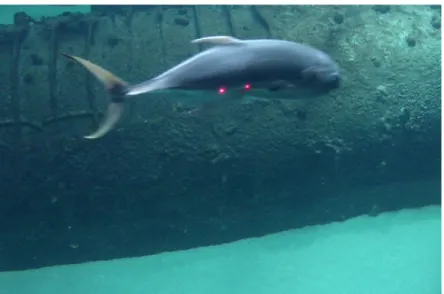
To match acoustic return to a specific fish species and length, we deployed a downward-facing 650 Sea-Drop Color Seaviewer camera with the transducer to record digital video of fish that passed through the beam. The Seaviewer camera was attached to the same PVC pipe as the transducer, with the lens of the camera even with the face of the transducer to produce a video that showed the dorsal-aspect of the fish as they swam under the beam of the transducer (i.e., the visual representation of what the transducer was acoustically recording). The video from the Seaviewer camera was fed live to a monitor and was recorded. The clock on the digital video recorder was then synchronized with the clock on the SBES to permit pairing of acoustic and video observations (see Analysis section).
Length estimation
the video to estimate fish lengths. An image calibration tool in ImageJ was used to set the distance between the two lasers in the frame to a distance of 10 cm, converting Euclidean distance between two pixels to real-world distances (in cm). We used the measure tool in ImageJ and drew a line to estimate fork length. In cases where the species did not have a distinguishable fork in the caudal fin (Epinephelus morio, Mycteroperca microlepis, Sciaenops ocellatus), we used total length.
The laser-sizing method was used to match lengths for individual fish. This way we matched specific individuals with measured length to a corresponding acoustic return. However, this method only allowed us to match individual target strength to single fish of known length five times during our experiments. For the species that we could not assign individual TS and length, we had to compute the mean size and mean TS for the species. Our experimental units were a combination of species-specific averages and measurements from individual fish. We collected supplementary lengths using a GoPro Hero 2 camera attached to the laser caliper, which allowed us to move freely around the edge of the tank. The average length of each fish species was
calculated by compiling measurements of individual fish from sequential frames of video in which the 10 cm calibration lasers were clearly observable on the fish. Since we had multiple length measurements and return signals for several individuals of a given species, these datapoints had associated error bars in both the X- and Y-directions.
Analysis
Raw data from the SBES was processed with the Echoview hydroacousitc data-processing application developed for use by fisheries scientists and environmental managers (ref Echoview version 5.4, http://www.echoview.com). The program visualizes, processes, and characterizes acoustic data from echo sounders and sonar systems with user-definable algorithms. The single target detection algorithm in Echoview calculates the TS of fish at each ping. Sequential echoes for each fish were grouped manually and assigned to a specific individual. Each fish was assigned a depth below the water surface and average target strength. We also used the media module in Echoview to import and synchronize video from the Seaviewer camera with the acoustic data.
After the average target strength was calculated and matched to either a species or individual fish, the data was exported into MS Excel. The average target strength per species was paired with the average length measurement per species as single data points in our model. We also included the paired length and signal strength data from the five known individuals in our model. We used the logarithmic-based equation from Love (1971) to describe the TS-length functional relationship.
where TS is target strength (dB), A and B are parameters to be fit, and L is fork or total length (cm). Using this general equation, we used Solver in Excel to estimate the parameter values that provided the best fit for the functional relationship between fish length and target strength.
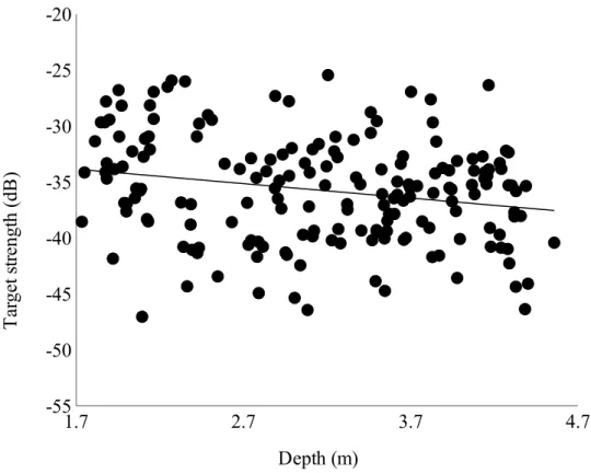
Data were further analyzed for factors that might affect the target strength. We hypothesized that there would be a general decrease in TS with depth. This may be due to factors such as the change in beam width with depth, fish behavior (i.e. position preference in the water column), and pressure change with depth. We tested the potential depth bias on TS by examining how TS differed across depths for all 181 returns. In order to determine whether the potential depth effect was due to fish behavior (i.e., smaller or larger fish being more strongly associated with the bottom or surface), we examined the relationship between depth and fish length. Statistical analysis of the relationship between TS and depth and fish length and depth was completed in R 2.14.1.
Results
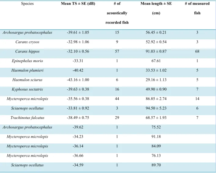
During the course of our experiment, we recorded a total of 418 acoustic returns from 181 individual reef fish from ten different species: Archosargus probatocephalus, Caranx crysos,
Caranx hippos, Epinephelus morio, Haemulon plumieri, Haemulon sciurus, Kyphosus sectatrix,
Species Mean TS ± SE (dB) # of
acoustically
recorded fish
Mean length ± SE
(cm)
# of measured
fish
Archosargus probatocephalus -39.61 ± 1.05 15 56.45 ± 0.21 3
Caranx crysos -32.98 ± 1.06 9 52.92 ± 0.54 3
Caranx hippos -32.10 ± 0.56 57 91.03 ± 0.87 68
Epinephelus morio -33.31 1 67.61 1
Haemulon plumieri -40.42 1 33.53 ± 1.02 5
Haemulon sciurus -43.16 ± 1.00 6 29.16 ± 1.13 5
Kyphosus sectatrix -39.63 ± 0.38 16 49.90 ± 0.90 7
Mycteroperca microlepis -35.56 ± 0.38 44 86.85 ± 2.74 14
Sciaenops ocellatus -33.81 ± 0.92 3 94.50 ± 5.23 6
Trachinotus falcatus -38.49 ± 0.75 29 68.57 ± 1.93 7
Archosargus probatocephalus -39.62 1 75.52
Mycteroperca microlepis -34.23 1 91.18
Mycteroperca microlepis -36.14 1 84.09
Mycteroperca microlepis -36.66 1 76.13
Sciaenops ocellatus -34.59 1 89.70
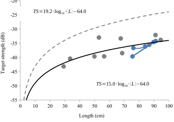
The logarithmic equation was fit to our average TS per species and five individual fish versus average length. Love’s general equation with our calculated parameters fits the data well (R2 =
0.53) (Fig. 2). We estimated parameter A as 15.0 and parameter B as – 64.0, for the resulting equation:
TS=15.0∙log10∙(L)−64.0.
0 10 20 30 40 50 60 70 80 90 100 -55
-50 -45 -40 -35 -30 -25 -20
Length (cm)
T
ar
ge
t s
tr
en
gt
h
(d
B
)
We qualitatively compared our model to that currently used in acoustic surveys in coral reef ecosystems (Kracker et al., 2011 and Costa et al., 2014) by plotting both regression lines with our data (Fig. 3) and comparing the parameter estimates. The currently-used TS-length equation (Love, 1971 and Brandt et al., 1991) has parameter A = 19.2 and B = -64.0. Parameter B, the y-intercept, is the same in both the currently-used equation and our model when corrected for frequency. Parameter A from the currently used model, however, is 28% larger than our estimated parameter (A = 15.0). Parameter A controls the horizontal asymptote of the curve. With a larger parameter A (or horizontal asymptote), the corresponding length per specific TS is
Fig. 2: Logarithmic functional relationship between fish length (cm) and target strength (dB) for individuals within a species (grey points) and the five uniquely identified individuals (black points). Standard error is represented by the
horizontal and vertical error bars on each data point.
smaller. Therefore, in comparison, the currently-used equation will give smaller estimates of fish length per target strength than our estimated equation.
0 10 20 30 40 50 60 70 80 90 100
-55 -50 -45 -40 -35 -30 -25 -20
Length (cm)
T
ar
ge
t s
tr
en
gt
h
(d
B
)
We tested the potential depth bias on TS by examining how TS differed across depths for all 181 returns. There was a significant negative relationship between TS and depth (p < 0.005),
suggesting that target strength decreases with increasing depth (Fig. 4). TS=19.2∙log10∙(L)−64.0
TS=15.0∙log10∙(L)−64.0
1.7 2.7 3.7 4.7 -55
-50 -45 -40 -35 -30 -25 -20
Depth (m)
T
ar
ge
t s
tr
en
gt
h
(d
B
)
We examined the relationship between depth and fish length to determine whether the potential depth effect was due to smaller fish having a preference for deeper parts of the tank. Although there was evidence of our hypothesized trend of decreasing length with increasing depth, the effect was not significant (p = 0.1735). Therefore, it is unlikely that size-specific depth distributions biased our TS measurements.
Because the depth effect was not due to a general pattern of size-specific fish preference for a particular depth, we then tested whether there was a fish size-depth effect for each species. For all but two species, there was no significant trend of the effect of depth on TS. For species A. probatocephalus, C. hippos, E. mario, H. plumier, H. sciurus, M. mincrolepis, S. ocellatus, and
T. falcatus there was no significant effect of depth on TS (p > 0.05). For C. crysos and K.
sectatrix there was a significant (p < 0.05) effect of depth on measured TS, however the patterns were opposite for the two species. Caranx crysos showed increased TS with depth (Fig. 5A), which was opposite our original hypothesis, whereas Kyphosus sectatrix showed decreased TS with depth (Fig. 5B).
1.7 2.2 2.7 3.2 3.7 4.2
-45 -40 -35 -30 -25
1.7 2.2 2.7 3.2 3.7 4.2
-45 -40 -35 -30 -25 Discussion
Acoustic surveys require accurate information on the functional relationship between fish target strength (TS) and fish length to estimate the abundance, size distribution, and biomass of fish populations. Therefore, there is a need for accurate TS-length regression models. The previous model, and its parameters, was originally developed using data from several fish species in the Great Lakes (Acoustics Unpacked, 2014) and qualitatively compared to a limited sample of TS
Fig. 5: Affect of depth on TS for (A) Caranx crysos; p < 0.005 and for (B)
Kyphosus sectatrix; p < 0.05.
and length data from reef fish (Johnston et al., 2006) The model has been used in surveys to map the distribution of reef fish in the US Caribbean coral reef ecosystems (Kracker et al., 2011 and Costa et al., 2013). Although this model is used in marine surveys, it was not originally
developed using data from marine fish species. This experiment gathered TS-length relationship data for Mid-Atlantic reef fish species, with the purpose of developing an accurate regression model for reef fish.
Comparing TS-length models
We chose to compare our model with that developed by Brandt el al. (1996) because that model has been used in bioaccoustic surveys in reef ecosystems (Kracker et al., 2011 and Costa et al., 2013). The comparison between the two equations reveals a difference in the equation
parameters. It appears that our model may be a more accurate model for reef fish. In general, when using the new model, estimates of fish length are consistently larger for a given TS.
Several problems arise from using the currently-used equation, including the possible exclusion of smaller fish of reproductive age and size from these distribution maps as well as an
underestimate of the size of spawning aggregations and population biomass. If using the new model, these size classes may have to be adjusted as fish with an estimated length with a given TS may have a different estimated length using another model. The currently-used equation may underestimate fish length for a given TS and would potentially bias size distribution and biomass estimates of fish populations. For example, this calculation shows how the corresponding TS to the minimum size of a “large fish” would vary depending on the model used: using the currently model, a TS of 35.92 dB represents a fish that is 29 cm, while using the new model, a TS of -42.06 dB represents a fish that is 29 cm. If a study constructed length frequency distributions for a reef fish using Love’s (1971) equation the true distribution would actually be shifted towards the right of what was estimated. This would alter what maps show as the distribution of “large fish” and thus would have implications for marine spatial management of these fisheries. Since biomass estimates will be based on these length frequency distributions, the biomass estimates would also be biased toward estimates of lower biomass.
Sources of variation in individual target strength
Fish length, tilt (vertically and horizontally), and depth influence the shape or orientation of the swimbladder and consequently have an effect on TS, but the relative contribution of each factor is difficult to isolate and quantify (Hazen and Horne, 2003). In this experiment we were able to analyze our TS data with length and depth, but did not examine fish orientation and the
subsequent affect on TS. Further analysis and experimentation should examine the effect of tilt on TS in this study and in general.
As pressure increases with depth, the swimbladder volume decreases due to pressure and the TS of the fish also decreases (Hazen and Horne, 2003). According to Hazen and Horne (2003), the largest rate of decrease in estimated fish length occurs within the first 50 m of the water column, therefore we hypothesized that this effect could be measured in 5 m. Future studies should collect data down to greater depths in controlled environments to quantify this change with depth to include in models. We found that within 3 m there was a significant decrease in TS with depth. We wanted to find the mechanism for this change, so we examined how TS was changing with depth for each species. We analyzed change in TS with depth for each of the ten species and found two species for which there was a significant change with depth. However, the two species showed opposite patterns: Caranx crysos showed increased TS with depth and Kyphosus
sectatrix showed decreased TS with depth.
Another possible mechanism to explain the differing TS with depth might be the schooling behavior observed in this experiment for Caranx crysos. When organism densities are very high, multiple scattering (echoes that have scattered off multiple individuals before returning to the transducer) and shadowing have non-linear effects and make TS hard to predict (Parker-Stetter, 2009; MacLennan, 1990; Toresen, 1991). This effect might have resulted in the lower TS
crysos, where the narrow beam may not fully ensonify the swimbladder and provide an accurate backscatter.
The sound beam from the echo sounder is conical in shape and thus as length of the beam increases with depth, the width and sampling volume of the beam also increase. Therefore, fish in deeper water will be overrepresented in the data relative to their contribution to overall density (Parker-Stetter, 2009). It is the case that in many lakes for example, larger fish are found deeper and will be overrepresented in a TS distribution derived from the whole water column (Parker-Stetter, 2009). The same could be possible in our experiment, but it should also be noted that the shallow depth limited the beam width and therefore it is possible that only parts of the fish towards the top of the water column were in the sound beam. The general pattern of
overrepresentation of TS distribution might affect length and biomass estimates as would partial ensonification by a limited beam width.
This study attempted to address factors that cause variation in target strength by examining how fish depth and behavior may influence the return strength of acoustic backscatter. The general TS-length model for reef fish that was developed in this study was compared to the currently-used model. The implication for the findings from this study is improved interpretation of fish distribution, population size distribution, and biomass estimates from acoustic surveys in reef ecosystems.
Acknowledgements
Hill for guidance in the writing and presentation of this research, Marc Alperin for his involvement in the Honors Thesis defense process, the NOAA Office of Education and the Hollings Scholarship program for funding this project, the senior honors thesis program through Honors Carolina, and the NC Aquarium at Pine Knoll Shores for providing the study site.
References
Acoustics unpacked, a general guide for deriving abundance estimates form hydroacoustic data.
Retrieved April/06, 2014, from http://www.acousticsunpacked.org/acoustics/
Brandt, S. B., Mason, D. M., Patrick, E. V., Argyle, R. L., Wells, L., Unger, P. A., et al. (1991). Acoustic measures of the abundance and size of pelagic planktivores in Lake
Michigan. Canadian Journal of Fisheries and Aquatic Sciences, 48(5), 894-908. Clay, C. S., & Horne, J. K. (1994). Acoustic models of fish: The Atlantic cod (Gadus
morhua). The Journal of the Acoustical Society of America, 96(3), 1661-1668. Costa B, Taylor JC, Kracker L, Battista T, Pittman S (2014) Mapping Reef Fish and the
Seascape: Using Acoustics and Spatial Modeling to Guide Coastal Management. PLoS ONE 9(1): e85555. doi: 10.1371/journal.pone.0085555
Echoview sound knowledge. (2014). Retrieved April/06, 2014, from http://www.echoview.com Foote, K. G. (1987). Fish target strengths for use in echo integrator surveys. The Journal of the
Acoustical Society of America, 82(3), 981-987.
Hazen, E. L., & Horne, J. K. (2003). A method for evaluating the effects of biological factors on fish target strength. ICES Journal of Marine Science: Journal Du Conseil, 60(3), 555-562. "ImageJ, Image Processing and Analysis in Java." ImageJ. N.p., n.d. Web. 25 Apr. 2014. <http://
imagej.nih.gov/ij/>.
Johnston, S. V., Rivera, J. A., Rosario, A., Timko, M. A., Nealson, P. A., & Kumagai, K. K. (2006). Hydroacoustic evaluation of spawning red hind (epinephelus guttatus) aggregations along the coast of puerto rico in 2002 and 2003.
Kracker, L. M. (2011). Integration of fisheries acoustics surveys and bathymetric mapping to characterize midwater-seafloor habitats of US virgin islands and puerto rico
(2008-2010) NOAA, National Ocean Service, National Centers for Coastal Ocean Science, Center for Coastal Environmental Health and Biomolecular Research.
Love, R. H. (2005). Dorsal‐aspect target strength of an individual fish. The Journal of the Acoustical Society of America, 49(3B), 816-823.
MacLennan, D. N. (1990). Acoustical measurement of fish abundance. The Journal of the Acoustical Society of America, 87(1), 1-15.
Office of Ocean Exploration and Research, National Oceanic and Atmospheric Administration (NOAA). (2013). Ocean Explorer SONAR. Retrieved April/06, 2014, from
http://oceanexplorer.noaa.gov/technology/tools/sonar/sonar.html
Parker-Stetter, S. L. (2009). Standard operating procedures for fisheries acoustic surveys in the great lakes.
Reeder, D. B., Jech, J. M., & Stanton, T. K. (2004). Broadband acoustic backscatter and high-resolution morphology of fish: Measurement and modeling. The Journal of the Acoustical Society of America, 116(2), 747-761.
Rudstam, L. G., Hansson, S., Lindem, T., & Einhouse, D. W. (1999). Comparison of target strength distributions and fish densities obtained with split and single beam echo sounders. Fisheries Research, 42(3), 207-214.
Simmonds, E., & MacLennan, D. Oxford: Blackwell science; 2005. Fisheries Acoustics: Theory and Practice, 437.
Toresen, R. (1991). Absorption of acoustic energy in dense herring schools studied by the attenuation in the bottom echo signal. Fisheries Research, 10(3), 317-327.