by Jacob Bogerd
Abstract
Although genetic information in the cell is stored in DNA, the RNA transcripts obtained from DNA indicate which genes are actively transcribed. Modern high-throughput sequencing techniques allow accurate sequencing of short RNA fragments, which may then be aligned to a reference genome. These alignments can be summarized by constructing a "splice graph", in which nodes represent genomic coordinates and edges represent sequences that are retained or spliced out of observed transcripts. Each full-length transcript corresponds to a path through the graph. I have written software to build a splice graph from a collection of short reads aligned to a reference genome. This software incorporates variants observed relative to the reference genome as additional paths. I have also written tools to manipulate and traverse such graphs. An application of this graph is correction of noisy full-length RNA transcripts. Such a transcript may be aligned to paths through the graph in order to identify its original sequence.
Background
Genetic information in the cell is stored in the nucleus in the form of DNA. RNA transcription is the process by which messenger RNA is produced from this DNA. This mRNA may then leave the nucleus of the cell. Once outside of the nucleus, it can be translated into a functional protein. The set of all mRNA transcripts in a given cell is called the transcriptome. By analyzing the contents of the transcriptome, we can determine what genes are transcribed in a cell. The relative abundance of each transcript also tells us to what extent each observed gene is expressed.
When a sequence of DNA is transcribed, a complementary sequence of mRNA is
produced. This transcript then undergoes mRNA splicing. Splicing is a process by which specific intervals are removed from the transcript, and the retained portions of the sequence on either side of the interval are ligated together. The spliced out sequences are called introns, and the retained sequences are called exons.
An individual gene may produce many different RNA transcripts through the process of alternative splicing. Sometimes an interval in a transcript that is normally an intron may actually be retained, or an interval that is normally an exon may be spliced out. Another common possibility is that a splice donor site that normally pairs with a specific splice acceptor site may pair with an alternative acceptor site, or vice versa. Alternative splicing occurs regularly, and can lead to an increased variety of proteins produced from a set of genes.
two major high-throughput sequencing technologies that we will discuss, each with different characteristics. Illumina manufactures a sequencer that takes a sequencing-by-synthesis approach. This sequencer produces short reads of up to 150 bases in length (Quail 2). These reads are high quality, with an error rate of less than 1% (Quail 2). Pacific Biosciences makes a sequencer that performs single molecule real time sequencing. This produces long reads of 1500 bases in length on average (Quail 2). The tradeoff is that these reads are of significantly lower quality, with an error rate of around 13% (Quail 2). By making use of both of these sequencing technologies, we can make an appropriate tradeoff between read length and read quality.
The data obtained from RNA sequencing describes the sequence of individual
transcripts. These sequences can then be aligned to a reference genome. By doing so, we can determine the location of each transcript in the genome. Well known algorithms for alignment of DNA sequences exist, but they may not be sufficient to align a spliced RNA transcript to the genome. A standard alignment algorithm can be used to determine a starting coordinate for the alignment and a sequence of matched, mismatched, inserted and deleted bases that aligns the two sequences with minimum edit distance. When aligning an RNA transcript in this
fashion, spliced intervals may be penalized as massive deletions, hiding the true alignment from the results. To account for this, a gapped alignment algorithm such as MapSplice can be used (Wang). MapSplice performs the alignment in a way that takes splices into account, and can even detect novel splice sites.
Overview of the Splice Graph
We will propose a graph representation of a set of aligned RNA transcripts. We will refer to this representation as a splice graph. The splice graph builds upon the ACT-Graph proposed by Singh et al. by adding observed nucleotide counts at each position, a more flexible graph representation, and variant calling (Singh 2634). Such a graph representation can effectively compress a large set of aligned transcripts because overlapping sequences are condensed into a single edge (Singh 2635). Additionally, we describe a procedure to construct such a splice graph from aligned RNA sequence data.
a SNP edge. This ensures that we only include variants in the graph when we can confidently claim that they are true variants and not random sequencing errors.
Figure 1 – A splice graph with three exons and two introns. Exon edges are represented by solid lines, splice edges are represented by dashed lines.
The coverage at a specific genomic position is the number of exons that include that position in a gapped alignment. The weight of an exon edge is the average coverage over the genomic interval spanned by that edge. Such an edge is also labeled with individual nucleotide coverage values for each genomic position it covers. This additional detailed coverage
information simplifies recalculation of average coverage when performing a union of splice graphs. The weight of a splice, insertion, deletion, or SNP edge is the number of reads that include the represented feature.
Edges are directed from lower to higher genomic coordinates. The low coordinate is always inclusive, and the high coordinate is always exclusive. For exon edges, this means that the retained sequence extends from the low coordinate to the position just before the high coordinate. For splice edges, the spliced out interval extends from the low coordinate to the position just before the high coordinate. SNP edges extend from the position of the SNP to the next coordinate. This choice of coordinates allows for parallel edges. For example, a splice may be observed across an interval in some reads, but other reads may indicate that the interval was actually retained. In this case, an exon edge and a splice edge will run in parallel for the duration of the interval.
All edges are tagged with additional attributes. Both exon and SNP edges are tagged with an associated sequence. For an exon edge, the sequence is obtained from the
corresponding interval in a standard reference genome. For a SNP edge, the sequence is the variant base associated with the edge.
Edges are also labeled to indicate the direction of transcription. Initially during the graph construction, only splices have direction information, as this is inferred from the orientation of asymmetric canonical splice sites. Once the graph structure is complete, this direction
information is propagated from splices to adjacent edges. This representation simplifies the work needed to recalculate transcription direction when performing a union of splice graphs, and enables simple traversal in either direction.
Edges between the same pair of coordinates are differentiated by a multigraph key. For SNP edges, this multigraph key is the letter representing the variant base for that edge. For exon edges, the multigraph key is “exon”. For splice edges, the multigraph key is “splice”. Thus, all possible edges between a pair of coordinates are differentiated.
Splice Graph Construction Procedure
We can construct such a splice graph from aligned RNA sequence data. First, we must obtain accurate RNA short read sequence data, such as the output of an Illumina sequencer. We can then perform a gapped alignment of this sequence data to a reference genome with a program such as MapSplice in order to produce a BAM formatted set of aligned reads. The BAM format is a binary version of the SAM format, which is designed to store alignments of reads to reference sequences (Li 2078). This aligned sequence data will be the input to the graph construction procedure.
mismatches, and deletions in the aligned read. If we see an interval in which the reference is recorded as skipped, this will correspond to a splice, and we may record it as such (Li 2078). Additionally, the read may contain information about the observed direction of transcription, as inferred from any well-known asymmetric splice sites it spans. We record these splices by inserting them as splice edges in a new directed multigraph. If transcription direction
information is present, the splices will be tagged with it. In the future, this step could be made optional if a list of splices were provided as an additional input to the graph construction software. Additionally, if transcription direction information is not provided by the gapped aligner upstream in the process, that information could be determined at this time by inspection for canonical splice sites.
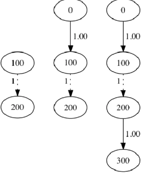
Once we have a skeleton of the splice graph consisting solely of splice edges, we are ready to perform a pileup iteration of the aligned reads, as illustrated in Figure 3. In a pileup iteration we iterate over all coordinates in the genome with at least one aligned read. At each position we inspect all of the bases that are part of an aligned read at that position. As we traverse the aligned reads, we maintain state representing an unfinished exon edge. This working edge begins when we reach a position with nonzero coverage. There are two possible termination conditions for an exon edge that will cause the finished edge to be written to the splice graph. An edge will be terminated if coverage drops below a configurable threshold. An edge may also be terminated if the current genomic coordinate in the iteration is already in the graph as an incoming or outgoing splice site. In the latter case, we may immediately resume work on an exon edge if coverage is above the threshold. At each position with sufficient coverage, we will also perform a variant calling procedure, and insert SNP edges as necessary.
Figure 3 – Incremental construction of a splice graph. In the left image, we see the initial graph consisting solely of splice edges. In the center we see the graph after the first exon has been flushed to the graph upon hitting a splice coordinate. On the right
The bases aligned to a given position may or may not agree with the reference genome. The problem of variant calling is to decide whether this is due to sequencing error or the observation of an actual variant base. We will perform this variant calling procedure at each position in the genome with nonzero coverage. As input to this procedure, we are given 𝑛 nucleotides that agree with the reference at this position and 𝑘 occurrences of other nucleotides. If 𝑘 is 0 then we are done, because all observed nucleotides agree with the reference genome.
If 𝑘 is greater than 0, we must perform a significance test. Our null hypothesis is that no SNP is present at this position, and all deviations from the reference are due to random chance. The alternative hypothesis is that there is a SNP at this position. We will assume that the
sequencer makes errors with a constant error probability 𝑝 when reading a nucleotide. First, we wish to determine the probability that 𝑘 − 1 or fewer sequencing errors occurred at this
position. This is a cumulative binomial probability, as shown in Equation 1.
𝑃𝑆𝑁𝑃 = ∑ (𝑛
𝑖) (1 − 𝑝)
𝑛−𝑖𝑝𝑖 𝑘−1
𝑖=0
Equation 1 – The probability that k-1 or fewer non-reference bases are in error. This is the probability that we have observed a true variant, and not just random sequencing errors.
Using this value, we can determine the probability that no SNP is present at this position by taking the complement of the previous probability. This is shown in Equation 2.
𝑃𝑒𝑟𝑟𝑜𝑟 = 1 − ∑ (𝑛
𝑖) (1 − 𝑝)
𝑛−𝑖𝑝𝑖 𝑘−1
𝑖=0
Equation 2 – The probability that observed variants are simply due to random sequencing errors.
If 𝑃𝑒𝑟𝑟𝑜𝑟 is less than some significance cutoff 𝛼, we will reject the null hypothesis that
there is no SNP present at this position. If this test leads us to call a SNP, the nucleotide we will report as the variant will be the non-reference base with the most occurrences at the current genomic position.
After completing the pileup iteration, information about transcription direction must be propagated among the edges of the graph. Initially, only splice edges have direction
information associated with them. A simple approach to this problem is to propagate information within weakly connected components in the graph. These components roughly correspond to observed genes. By iterating over all splices in a component, we can determine which direction or directions of transcription were observed for a given gene. That information can then be assigned to each edge in the component. There is potential for confusion in the case where two genes transcribed in opposite directions overlap briefly at one end. In the scheme described previously, both genes would be recorded as transcribed in both directions.
transcription direction information as much as possible. I have implemented the simple approach in my splice graph software, but an implementation of the latter approach would be possible in the future.
Applications
One possible application of a splice graph is long read correction. Although long reads can cover larger transcripts, they have a very high error rate (Quail 2). It would be desirable to correct these noisy sequences. Our splice graphs are built from short reads, which have a much lower error rate than long reads. If we could align a long read to a path through a splice graph built from shorts reads from the same sample, we could then read off the sequences associated with that path to obtain a more accurate sequence. Significant variants will also be included in the resulting sequence because the graph contains edges corresponding to the observed SNPs.
In order to make this application work, we need to be able to align a transcript to a path through a splice graph. First, we must find a starting point for the alignment. We can do so by aligning short subsequences of the long read to each exon edge in the splice graph until we find a near match. We can then traverse paths outward from the starting edge within a weakly connected component of the graph, essentially performing a breadth-first search. As we
incorporate edges, we perform successive alignments of the transcript against the sequences of these new edges. If any given path exceeds a local error bound in the alignment, it may be discarded as an unlikely alignment. Once this procedure is completed, we will have some subset of paths through the graph remaining. One of these with the minimum edit distance to the transcript will be chosen as the correct alignment. The sequence of that path should be the corrected sequence of the long read, including called variants.
Overview of Additional Software
In addition to the core software to construct a splice graph, I have written tools to perform various operations on splice graphs. Some of these tools can be used to work with an existing graph. Other tools may be used to construct a new graph from an existing graph or set of graphs. By using tools such as this, we can sometimes build new splice graphs without having to consult the original alignments. We can save significant amounts of time by modifying
existing graphs instead of constructing new ones whenever possible.
One simple graph operation I have implemented is the conversion of a splice graph from one format to another. This allows the storage representation of a graph to be changed after it is created. This could be used to write graphs in a compact format, but then rewrite them in a human-readable format if necessary.
unique to each of the input graphs. This could be used to verify a splice graph against an existing splice graph, or to compare splice graphs constructed from different samples.
Additionally, I wrote a procedure to visualize a splice graph using Graphviz. This was particularly useful for debugging purposes. I also used this visualization procedure to generate all of the splice graph illustrations in this paper.
In order to simplify the development of a long read alignment procedure, I implemented an interface for the traversal of an existing splice graph. This interface provides methods to traverse the graph in either direction from a given starting edge. This is made simple by the directedness of the graph. All edges are directed from low to high genomic coordinates. Therefore, to traverse the graph in the increasing direction, we follow outgoing edges, and to traverse it in the decreasing direction, we follow incoming edges. By providing a higher-level interface to the graph, we can offer different views of the data and simplify specific applications of the graph.
In order to support the merging of two existing splice graphs, I have implemented a splice graph union procedure. The standard definition of a graph union is to take the union of the set of nodes, and the union of the set of edges. This definition is not sufficient here. The way we have defined a splice graph requires that exon edges correspond to disjoint genomic intervals, and a standard graph union would be able to violate this property. In order to correctly perform a splice graph union, we can first combine the splice edges from each of the input graphs in a new graph, adding together the weights of corresponding edges. We may then sort exon edges from both graphs by their starting coordinate. We sequentially insert these edges into the graph, merging with existing edges when overlap occurs. If we hit an incoming or outgoing splice junction, we can split the exon edge at that coordinate. When exon edges are merged or split, we need to recalculate their weights. The weight of an exon edge is the average coverage observed over that genomic interval. We can determine the new average coverage without consulting the original alignment file by virtue of the fact that we’ve saved coverage information at each genomic coordinate as an attribute on each exon edge. Coverage can then be added together at overlapping positions, and average coverage may be
recomputed. This procedure allows us to join splice graphs from multiple samples, or to break the work needed to construct a splice graph into smaller units for improved parallelism.
Future Work
upstream in the process. This would enable a larger variety of gapped aligners to be used when generating the input for the graph construction.
Another area for improvement is the procedure for propagation of transcription direction tags from splice edges to the rest of the graph. There is currently possibility for ambiguity if two genes overlap slightly on opposite strands. By performing the more
sophisticated direction propagation procedure described earlier, we can reduce the scope of this ambiguous information.
Due to limitations of the BAM format, this software is unable to handle chromosome fusion events or splices that are performed backwards relative to the direction of transcription. The BAM format uses CIGAR strings to represent the detailed alignment of each read. The linear nature of CIGAR strings limits splice detection to forward splices. If the format were modified to include a way to express reverse splices and chromosomal fusion events, those could be
Works Cited
Li, H., B. Handsaker, A. Wysoker, T. Fennell, J. Ruan, N. Homer, G. Marth, G. Abecasis, and R. Durbin. "The Sequence Alignment/Map Format and SAMtools." Bioinformatics 25.16 (2009): 2078-079. Web.
Quail, Michael, Miriam E. Smith, Paul Coupland, Thomas D. Otto, Simon R. Harris, Thomas R. Connor, Anna Bertoni, Harold P. Swerdlow, and Yong Gu. "A Tale of Three Next Generation Sequencing Platforms: Comparison of Ion Torrent, Pacific Biosciences and Illumina MiSeq Sequencers." BMC Genomics 13.1 (2012): 341. Web.
Singh, D., C. F. Orellana, Y. Hu, C. D. Jones, Y. Liu, D. Y. Chiang, J. Liu, and J. F. Prins. "FDM: A Graph-based Statistical Method to Detect Differential Transcription Using RNA-seq Data." Bioinformatics 27.19 (2011): 2633-640. Web.