Available online at www.cuijca.com
International Journal of Computational Analysis Vol (3), No. (2), pp. 26-35
* Corresponding author: E-mail address: [email protected]
HYBRID-BLOCK NUMERICAL METHOD FOR SOLVING SECOND ORDER ORDINARY DIFFERENTIAL EQUATIONS
Akeremale, Olusola Collins1,2, Kuboye, Olusola John3, Hoe Su Yeak.1, Augustine E. Abununyi2, Olaiju Segun1,4
1Department of Mathematical Sciences, Universiti Teknologi Malaysia, 81310, Skudai, Johor Bahru 2Department of Mathematics, Federal University Lafia, P.M.B 146, Nasarawa State, Nigeria 3Deparment of Mathematics, Federal University Oye, P.M.B 373, Ekiti State, Nigeria.
4Department of Mathematics and Statistics, Federal Polytechnics, Ilaro, P.M.B 50, Ogun State Nigeri
Corresponding author: [email protected]
Keywords: Power series, Collocation Points Interpolation point Second Order Differential Equations
Hybrid method Block method
ABSTRACT
In this work, a new hybrid block method for solving second order initial value problems of ordinary differential equations is developed. The derivation is achieved via multistep collocation approach with the use of approximated power series as the basis function. The discrete schemes and its derivatives are derived by evaluating the basis function at the grid and non-grid points which are used to form the block. In other to examine the efficiency of the new developed block method, it is applied to second order initial value problems and the results generated revealed the accuracy of the method over the existing methods. In this work, a new hybrid-block method for the solution of second order ordinary differential equation is developed using power series as the basis function. The developed scheme was used to solve some problems and the result compare with existing results to ascertain the superiority of the new method.
1. Introduction
In order to numerically and more accurately solve ordinary differential equations arising from science, social sciences and engineering, which most times do not have analytical solutions, many scholars had proposed several different numerical methods such as linear multistep, Euler, Runge-Kutta, hybrid and block methods depending on the nature and type of the differential equation to be solved. This work is focused on the numerical solution of second order differential equations.
𝑦′′ = 𝑓(𝑥, 𝑦, 𝑦′), 𝑦(𝑎) = 𝜇0, 𝑦(𝑎) = 𝜇1
𝑥 ∈ [𝑎, 𝑏] } (1) Though, these methods have their drawbacks but they can be circumvented or improve on as demonstrated in this work. 2. Literature Review
Many Scholars such ([6], [15,16], [9]) have suggested in the literature that a better alternative is to solve equation (1) directly without first reducing it to a system of first order ordinary differential equations.
Akeremale et al.
In [3], Awoyemi adopted the method and proposed a two-step hybrid multistep method with continuous coefficients for the solution of (1) based on collocation at selected grid points and using off-grid points to upgrade the order of the method and to provide one additional interpolation point and implemented on the hybrid predictor-corrector mode. Later, [10], hybrid method of order four was used to generate starting values for Numerov method. Many scholars which include but not limited to ([5],[8],[17]) had studied hybrid methods.
Fatunla [1,2] block method for special second order differential equations which was later developed by [4,7,11] was proposed. Parallel block methods in explicit and implicit for the solution of higher order differential equations where suitable interpolating polynomial was used to approximate the derivative function with a specified interval of integration was obtained. Many other scholars such as [12, 18], [13], [19] have adopted block methods where the derivative function was interpolated using Lagrange interpolation. These methods have largely focused on solving only special type ordinary differential equations with very few attempts in favour of (1). [14] and [20] have proposed five-step and four-step self-starting methods which adopt continuous linear multistep method to obtain finite difference methods applied respectively as a block for the direct solution of (1). Recently, ([21], [22], [23]) adopted hybrid-block method for the solution of second order ordinary differential equations and the results were found to be accurate and the scheme efficient compare to block methods.
While all the methods have their qualities and are very robust, we propose in this research, a new hybrid-block method that harness the qualities of the existing methods for the direct solution of (1).
3. Methodology
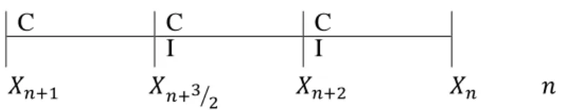
In this section, a new Hybrid-Block scheme for the solution of second order ordinary differential equation is developed. The
idea is to collocate the assumed function 𝑦(𝑥) at three points and interpolate at two points, which leaves us with five
equations. Thus, evaluating at these points to derive the method.
𝑋
𝑛+1𝑋
𝑛+3 2⁄
𝑋
𝑛+2𝑋
𝑛𝑛
Fig 1: collocation points
3.1. Derivation of the Hybrid-Block Method. Using power series as basis function we have
𝑦(𝑥) = ∑ 𝑎𝑖𝑥𝑖=
4
𝑖=0
𝑎0+ 𝑎1𝑥 + 𝑎2𝑥2+ 𝑎3𝑥3+ 𝑎4𝑥4 (3.1) Then
𝑦′(𝑥) = 𝑎
1+ 2𝑎2𝑥 + 3𝑎3𝑥2+ 4𝑎4𝑥3 (3.2)
C
C
C
28
𝑦′′(𝑥) = 2𝑎2+ 6𝑎3𝑥 + 12𝑎4𝑥2 (3.3)
Collocating equation (3.3) at 𝑥 = 𝑥𝑛, 𝑥 = 𝑥𝑛+1 and 𝑥 = 𝑥𝑛+2 we have
𝑦′′(𝑥
𝑛) = 2𝑎2+ 6𝑎3𝑥𝑛+ 12𝑎4𝑥𝑛2 (3.4) 𝑦′′(𝑥
𝑛+1) = 2𝑎2+ 6𝑎3𝑥𝑛+1+ 12𝑎4𝑥𝑛+12 (3.5) 𝑦′′(𝑥𝑛+2) = 2𝑎2+ 6𝑎3𝑥𝑛+2+ 12𝑎4𝑥𝑛+22 (3.6)
Also interpolating (3.1) at 𝑥 = 𝑥𝑛+1 and at 𝑥 = 𝑥𝑛+3 2⁄ we have
𝑦(𝑥𝑛+1) = 𝑎0+ 𝑎1𝑥𝑛+1+ 𝑎2𝑥𝑛+12 + 𝑎3𝑥𝑛+13 + 𝑎4𝑥𝑛+14 (3.7) 𝑦 (𝑥𝑛+3 2⁄ ) = 𝑎0+ 𝑎1𝑥𝑛+3 2⁄ + 𝑎2𝑥
𝑛+3 2⁄
2 + 𝑎3𝑥
𝑛+3 2⁄
3 + 𝑎4𝑥
𝑛+3 2⁄
4 (3.8)
The resulting matrix (of the form𝐴𝑥 = 𝑏) from the system of equations (3.4), (3.5), (3.6), (3.7) and (3.8) is
[
0 0 2 6𝑥𝑛 12𝑥𝑛2
0 0 2 6𝑥𝑛+1 12𝑥𝑛+12
0 0 2 6𝑥𝑛+2 12𝑥𝑛+22
1 𝑥𝑛+1 𝑥𝑛+12 𝑥𝑛+13 𝑥𝑛+14
1 𝑥𝑛+3 2⁄ 𝑥 𝑛+3 2⁄
2 𝑥
𝑛+3 2⁄
3 𝑥
𝑛+3 2⁄ 4 ][ 𝑎0 𝑎1 𝑎2 𝑎3 𝑎4]
= [
𝑦′′(𝑥𝑛) 𝑦′′(𝑥𝑛+1) 𝑦′′(𝑥𝑛+2)
𝑦(𝑥𝑛+1)
𝑦 (𝑥𝑛+3 2⁄ )]
(3.9)
Solving (3.9) using MatLab to find 𝑎𝑖, 𝑖 = 0,1,2,3,4 we have
𝑎0=[(21ℎ
4+ 77ℎ3𝑥
𝑛+ 96ℎ2𝑥𝑛2+ 48ℎ𝑥𝑛3+ 8𝑥𝑛4)𝑓𝑛]
192ℎ2 +
[(−3ℎ4− 11ℎ3𝑥
𝑛+ 16ℎ𝑥𝑛3+ 8𝑥𝑛4)𝑓𝑛+2]
192ℎ2
−[(−63ℎ
4− 87ℎ3𝑥
𝑛+ 32ℎ𝑥𝑛3+ 8𝑥𝑛4)𝑓𝑛+1]
96ℎ2 +
[(3ℎ + 2𝑥𝑛)𝑦𝑛+1]
ℎ −
[2(ℎ + 𝑥𝑛)𝑦𝑛+3 2⁄ ] ℎ
=(21ℎ
4+ 77ℎ3𝑥
𝑛+ 96ℎ2𝑥𝑛2+ 48ℎ𝑥𝑛3+ 8𝑥𝑛4)𝑓𝑛+ (−3ℎ4− 11ℎ3𝑥𝑛+ 16ℎ𝑥𝑛3+ 8𝑥𝑛4)𝑓𝑛+2
192ℎ2
−[(−63ℎ
4− 87ℎ3𝑥𝑛+ 32ℎ𝑥𝑛3+ 8𝑥𝑛4)𝑓
𝑛+1]
96ℎ2 +
(3ℎ + 2𝑥𝑛)𝑦𝑛+1− [2(ℎ + 𝑥𝑛)𝑦𝑛+3 2⁄]
ℎ =
21ℎ4𝑓
𝑛+ 77ℎ3𝑥𝑛𝑓𝑛+ 96ℎ2𝑥𝑛2𝑓𝑛+ 48ℎ𝑥𝑛3𝑓𝑛+ 8𝑥𝑛4𝑓𝑛− 3ℎ4𝑓𝑛+2− 11ℎ3𝑥𝑛𝑓𝑛+2+ 16ℎ𝑥𝑛3𝑓𝑛+2 +8𝑥𝑛4𝑓𝑛+2
192ℎ2
+63ℎ
4𝑓
𝑛+1+ 87ℎ3𝑥𝑛𝑓𝑛+1− 32ℎ𝑥𝑛3𝑓𝑛+1− 8𝑥𝑛4𝑓𝑛+1
96ℎ2 +
3ℎ𝑦𝑛+1+ 2𝑥𝑛𝑦𝑛+1− 2ℎ𝑦𝑛+3 2⁄ − 2𝑥𝑛𝑦𝑛+3 2⁄
ℎ
𝑎0=
ℎ4(21𝑓
𝑛− 3𝑓𝑛+2) + ℎ3𝑥𝑛(77𝑓𝑛− 11𝑓𝑛+2) + 96ℎ2𝑥𝑛2𝑓𝑛+ 𝑥𝑛3(48ℎ𝑓𝑛+ 𝑓𝑛+216ℎ) + 𝑥𝑛4(8𝑓𝑛+ 8𝑓𝑛+2)
192ℎ2
+63ℎ
4𝑓
𝑛+1+ 87ℎ3𝑥𝑛𝑓𝑛+1− 32ℎ𝑥𝑛3𝑓𝑛+1− 8𝑥𝑛4𝑓𝑛+1
96ℎ2 +
ℎ (3𝑦𝑛+1− 2𝑦𝑛+3 2⁄) + 𝑥𝑛(𝑦𝑛+1− 2𝑦𝑛+3 2⁄ )
ℎ
𝑎1=
2𝑦𝑛+3 2⁄
ℎ −
2𝑦𝑛+1
ℎ −
[(77ℎ3+ 192ℎ2𝑥
𝑛+ 144ℎ𝑥𝑛2+ 32𝑥𝑛3)𝑓𝑛]
192ℎ2 −
[(−11ℎ3+ 48ℎ𝑥
𝑛2+ 32𝑥𝑛3)𝑓𝑛+2]
192h2
+[(−87ℎ
3+ 96ℎ𝑥
𝑛2+ 32𝑥𝑛3)𝑓𝑛+1]
Akeremale et al.
=2 (𝑦𝑛+3 2⁄ − 𝑦𝑛+1)
ℎ −
77ℎ3𝑓
𝑛+ 192ℎ2𝑥𝑛𝑓𝑛+ 144ℎ𝑥𝑛2𝑓𝑛+ 32𝑥𝑛3𝑓𝑛
192ℎ2
+11ℎ
3𝑓
𝑛+2− 48ℎ𝑥𝑛2𝑓𝑛+2− 32𝑥𝑛3𝑓𝑛+2
192h2 −
87ℎ3𝑓
𝑛+1+ 96ℎ𝑥𝑛2𝑓𝑛+1+ 32𝑥𝑛3𝑓𝑛+1
96h2
𝑎1=
2 (𝑦𝑛+3 2⁄ − 𝑦𝑛+1)
ℎ −
ℎ3(77𝑓
𝑛− 11𝑓𝑛+2) + 192ℎ2𝑥𝑛𝑓𝑛+ ℎ𝑥𝑛2(144𝑓𝑛− 48𝑓𝑛+2) + 32𝑥𝑛3(𝑓𝑛− 𝑓𝑛+2)
192ℎ2
−87ℎ
3𝑓
𝑛+1+ 96ℎ𝑥𝑛2𝑓𝑛+1+ 32𝑥𝑛3𝑓𝑛+1
96h2
𝑎2=
(𝑥𝑛2+ ℎ𝑥𝑛)𝑓𝑛+2
4h2 −
[(𝑥𝑛2+ 2ℎ𝑥𝑛)𝑓
𝑛+1]
2h2 +
(2ℎ2+ 3ℎ𝑥𝑛+ 𝑥𝑛2𝑓𝑛)
4h2
=𝑥𝑛
2𝑓
𝑛+2+ ℎ𝑥𝑛𝑓𝑛+2+ 2ℎ2𝑓𝑛+ 3ℎ𝑥𝑛𝑓𝑛+ 𝑥𝑛2𝑓𝑛
4h2 −
𝑥𝑛2𝑓
𝑛+1− 2ℎ𝑥𝑛𝑓𝑛+1
2h2
𝑎2=
𝑥𝑛2(𝑓
𝑛+2+ 𝑓𝑛) + ℎ𝑥𝑛(𝑓𝑛+2+ 𝑓𝑛) + 𝑓𝑛2ℎ2
4h2 −
𝑥𝑛2𝑓
𝑛+1− 2ℎ𝑥𝑛𝑓𝑛+1
2h2
𝑎3=
(ℎ + 𝑥𝑛)𝑓𝑛+1
3h2 −
[(3ℎ + 2𝑥𝑛)𝑓𝑛]
12h2 −
[(ℎ + 2𝑥𝑛)𝑓𝑛+2]
12h2
=(ℎ + 𝑥𝑛)𝑓𝑛+1
3h2 −
3ℎ𝑓𝑛− 2𝑥𝑛𝑓𝑛− ℎ𝑓𝑛+2+ 2𝑥𝑛𝑓𝑛+2
12h2
𝑎3=(ℎ + 𝑥𝑛)𝑓𝑛+1
3h2 −
ℎ(3𝑓𝑛− 𝑓𝑛+2) − 2𝑥𝑛(𝑓𝑛+ 𝑓𝑛+2)
12h2
𝑎4=
𝑓𝑛
24h2−
𝑓𝑛+1
12h2+
𝑓𝑛+2
24h2
𝑎4=𝑓𝑛+ 𝑓𝑛+2
24h2 −
𝑓𝑛+1
12h2
Substituting 𝑎0, 𝑎1, 𝑎2, 𝑎3 𝑎𝑛𝑑 𝑎4 into (3.1)
𝑦(𝑥) =ℎ
4(21𝑓
𝑛− 3𝑓𝑛+2) + ℎ3𝑥𝑛(77𝑓𝑛− 11𝑓𝑛+2) + 96ℎ2𝑥𝑛2𝑓𝑛+ 𝑥𝑛3(48ℎ𝑓𝑛+ 16ℎ𝑓𝑛+2) + 𝑥𝑛4(8𝑓𝑛+ 8𝑓𝑛+2)
192ℎ2
+63ℎ
4𝑓
𝑛+1+ 87ℎ3𝑥𝑛𝑓𝑛+1− 32ℎ𝑥𝑛3𝑓𝑛+1− 8𝑥𝑛4𝑓𝑛+1
96ℎ2 +
ℎ (3𝑦𝑛+1− 2𝑦𝑛+3 2⁄ ) + 𝑥𝑛(𝑦𝑛+1− 2𝑦𝑛+3 2⁄ )
ℎ +
2𝑥 (𝑦𝑛+3 2⁄ − 𝑦𝑛+1)
ℎ
−𝑥ℎ
3(77𝑓
𝑛− 11𝑓𝑛+2) + 192ℎ2𝑥𝑛𝑥𝑓𝑛+ 𝑥ℎ𝑥𝑛2(144𝑓𝑛− 48𝑓𝑛+2) + 32𝑥𝑛3𝑥(𝑓𝑛− 𝑓𝑛+2)
192ℎ2
−87ℎ
3𝑥𝑓
𝑛+1+ 96ℎ𝑥𝑛2𝑥𝑓𝑛+1+ 32𝑥𝑛3𝑥𝑓𝑛+1
30
+𝑥
2𝑥
𝑛2(𝑓𝑛+2+ 𝑓𝑛) + 𝑥2ℎ𝑥𝑛(𝑓𝑛+2+ 𝑓𝑛) + 2𝑥2𝑓𝑛ℎ2
4h2 −
𝑥2𝑥
𝑛2𝑓𝑛+1− 2ℎ𝑥𝑛𝑥2𝑓𝑛+1
2h2 +
𝑥3(ℎ + 𝑥
𝑛)𝑓𝑛+1
3h2
−𝑥
3ℎ(3𝑓
𝑛− 𝑓𝑛+2) − 2𝑥𝑛𝑥3(𝑓𝑛+ 𝑓𝑛+2)
12h2 +
𝑥4𝑓
𝑛+ 𝑥4𝑓𝑛+2
24h2
−𝑥
4𝑓 𝑛+1
12h2 (3.10) let
𝑡 =𝑥 − (𝑥𝑛+𝑘−1)
ℎ Then,
𝑡 =𝑥 − (𝑥𝑛+2−1)
ℎ , 𝑤ℎ𝑒𝑛 𝑘 = 2
𝑡 =𝑥 − (𝑥𝑛+1)
ℎ =
𝑥 − (𝑥𝑛+ ℎ)
ℎ , 𝑠𝑖𝑛𝑐𝑒 𝑥𝑛+1= 𝑥𝑛+ ℎ
𝑡ℎ = 𝑥 − 𝑥𝑛− ℎ
𝑥 = 𝑡ℎ + 𝑥𝑛+ ℎ
𝑥 = 𝑥𝑛, 𝑤ℎ𝑒𝑛 𝑡 = −1
𝑥 = 𝑥𝑛+2= 𝑥𝑛+ 2ℎ, 𝑤ℎ𝑒𝑛 𝑡 = 1
From (3.10), the continuous scheme becomes
𝑦(𝑥𝑛) = 𝑦𝑛= 𝑦𝑛+1− 2𝑡𝑦𝑛+1+ 2𝑡𝑦𝑛+3 2⁄ +
(𝑡ℎ2𝑓
𝑛)
64 −
(23𝑡ℎ2𝑓
𝑛+1)
96 −
(5𝑡ℎ2𝑓
𝑛+2)
192 −
(𝑡3ℎ2𝑓 𝑛)
12 +
(𝑡2ℎ2𝑓 𝑛+1)
2 +
(𝑡4ℎ2𝑓 𝑛) 24
−(𝑡
4ℎ2𝑓 𝑛+1)
12 +
(𝑡3ℎ2𝑓 𝑛+2) 12
+(𝑡
4ℎ2𝑓 𝑛+2)
24 (3.11)
The derivative of (3.11) with respect to 𝑡 becomes
𝑦′(𝑥𝑛) = 𝑦𝑛′ =
ℎ(3𝑓𝑛− 46𝑓𝑛+1− 5𝑓𝑛+2+ 192𝑡𝑓𝑛+1− 48𝑡2𝑓𝑛+ 32𝑡3𝑓𝑛− 64𝑡3𝑓𝑛+1+ 48𝑡2𝑓𝑛+2+ 32𝑡3𝑓𝑛+2
192 −2𝑦𝑛+1− 2𝑦𝑛+3 2⁄
ℎ (3.12)
The discrete scheme when 𝑡 = −1
𝑦(𝑥𝑛) = 𝑦𝑛= 3𝑦𝑛+1− 2𝑦𝑛+3 2⁄ +
ℎ2
64[7𝑓𝑛+ 42𝑓𝑛+1− 𝑓𝑛+2] (3.13)
Also when 𝑡 = 1 we have
𝑦𝑛+2= 2𝑦𝑛+3 2⁄ − 𝑦𝑛+1− ℎ2
192[5𝑓𝑛− 34𝑓𝑛+1− 19𝑓𝑛+2] (3.14)
Evaluating the derivative of the discrete scheme at 𝑥 = 𝑥𝑛 and 𝑥 = 𝑥𝑛+2
At 𝑥 = 𝑥𝑛
𝑦𝑛′ =
−(2𝑦𝑛+1− 2𝑦𝑛+3 2⁄ )
ℎ −
(ℎ(77𝑓𝑛+ 174𝑓𝑛+1− 11𝑓𝑛+2))
192 ℎ𝑦𝑛′ = 2𝑦𝑛+3 2⁄ − 2𝑦𝑛+1−
ℎ2
192[77𝑓𝑛+ 174𝑓𝑛+1− 11𝑓𝑛+2] (3.15)
At 𝑥 = 𝑥𝑛+2
𝑦𝑛+2′ =−(2𝑦𝑛+1− 2𝑦𝑛+3 2⁄ )
ℎ +
(ℎ(82𝑓𝑛+1− 13𝑓𝑛+ 75𝑓𝑛+2))
Akeremale et al.
ℎ𝑦𝑛+2′ = 2𝑦𝑛+3 2⁄ − 2𝑦𝑛+1+ ℎ2
192[−13𝑓𝑛+ 82𝑓𝑛+1+ 72𝑓𝑛+2] (3.16)
Expressing (3.13), (3.14) and (3.15) in matrix form
[
−3 2 0
1 −2 1
2 −2 0
] [
𝑦𝑛+1
𝑦𝑛+3 2⁄
𝑦𝑛+2
]
= [
0 0 −1
0 0 0
0 0 0
] [ 𝑦𝑛−3 2⁄
𝑦𝑛−1
𝑦𝑛
] + ℎ [
0 0 0
0 0 0
0 0 −1
] [ 𝑦
𝑛−3 2⁄
′
𝑦𝑛−1′ 𝑦𝑛′
] + ℎ2
[
0 0 7⁄64
0 0 − 5 192⁄
0 0 − 77 192⁄ ]
[ 𝑓𝑛−3 2⁄
𝑓𝑛−1
𝑓𝑛 ]
+ ℎ2
[ 42
64
⁄ 0 − 1 64⁄
34 192
⁄ 0 19⁄192
− 174 192⁄ 0 11⁄192]
[
𝑓𝑛+1
𝑓𝑛+3 2⁄
𝑓𝑛+2
] (3.17)
Let 𝐴 = [
−3 2 0
1 −2 1
2 −2 0
] , 𝐵 = [
0 0 −1
0 0 0
0 0 0
] , 𝐶 = [
0 0 0
0 0 0
0 0 −1
],
𝐷 = [
0 0 7⁄64
0 0 − 5 192⁄
0 0 − 77 192⁄ ]
, 𝐸 = [
42 64
⁄ 0 − 1 64⁄
34 192
⁄ 0 19⁄192
− 174 192⁄ 0 11⁄192]
Then, 𝐴−1= [
−1 0 −1
−1 0 − 3 2⁄
−1 1 −2
]
Multiply through (3.19) by the inverse of A we have
[
1 0 0
0 1 0
0 0 1
] [ 𝑦𝑛+1 𝑦𝑛+3 2⁄
𝑦𝑛+2 ]
= [
0 0 1 0 0 1 0 0 1
] [ 𝑦𝑛−3 2⁄
𝑦𝑛−1
𝑦𝑛
] + ℎ [
0 0 1
0 0 3⁄2
0 0 2
] [ 𝑦
𝑛−3 2⁄
′
𝑦𝑛−1′ 𝑦𝑛′
] + ℎ2
[
0 0 7⁄24
0 0 63 128⁄
0 0 2⁄3 ]
[ 𝑓𝑛−3 2⁄
𝑓𝑛−1
𝑓𝑛 ]
+ ℎ2
[ 1
4
⁄ 0 − 1 24⁄
45 64
⁄ 0 − 9 128⁄
4 3
⁄ 0 0 ]
[
𝑓𝑛+1
𝑓𝑛+3 2⁄
𝑓𝑛+2
]
This implies that
𝑦𝑛+1= 𝑦𝑛+ ℎ𝑦𝑛′ + ℎ2[
7
24𝑓𝑛+
1
4𝑓𝑛+1−
1
24𝑓𝑛+2]
𝑦𝑛+3 2⁄ = 𝑦𝑛+ 3
2ℎ𝑦𝑛
′+ ℎ2[63
128𝑓𝑛+
45
64𝑓𝑛+1−
9
32
𝑦𝑛+2= 𝑦𝑛+ 2ℎ𝑦𝑛′+ ℎ2[
2
3𝑓𝑛+
4
3𝑓𝑛+2]
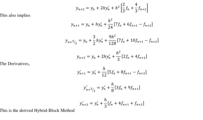
This also implies
𝑦𝑛+1= 𝑦𝑛+ ℎ𝑦𝑛′+
ℎ2
24[7𝑓𝑛+ 6𝑓𝑛+1− 𝑓𝑛+2]
𝑦𝑛+3 2⁄ = 𝑦𝑛+3
2ℎ𝑦𝑛
′+9ℎ 2
128[7𝑓𝑛+ 10𝑓𝑛+1− 𝑓𝑛+2]
𝑦𝑛+2= 𝑦𝑛+ 2ℎ𝑦𝑛′+
ℎ2
3 [2𝑓𝑛+ 4𝑓𝑛+2]
The Derivatives,
𝑦𝑛+1′ = 𝑦𝑛′+ ℎ
12[5𝑓𝑛+ 8𝑓𝑛+1− 𝑓𝑛+2]
𝑦 𝑛+3 2⁄
′ = 𝑦
𝑛′+ ℎ
8[3𝑓𝑛+ 9𝑓𝑛+1]
𝑦𝑛+2′ = 𝑦𝑛′+ℎ
3[𝑓𝑛+ 4𝑓𝑛+1+ 𝑓𝑛+2]
This is the derived Hybrid-Block Method 4. Numerical Examples
In order to ascertain the efficiency of this method, numerical experiment of some problems are performed and the results compared with that of the earlier literature.
4.1. Example 1
𝑦′′− 𝑥(𝑦′)2= 0, 𝑦(0), 𝑦′(0) =1
2, ℎ =
1 30, Exact solution;
𝑦(𝑥) = 1 +1
2𝐼𝑛 (
2 + 𝑥
2 − 𝑥)
Table 1: Comparison of the new method with Badmus and Yahaya. (2009) for solving Problem two. 𝑥
Theoretical Solution Computed Solution
Error
New method Badmus and Yahaya
(2009), 𝒌 = 𝟓
0.1 1.050041729278491400 1.050048113815469600 6.38 ∗ 10−06 5.89 ∗ 10−06
0.2 1.100335347731075600 1.100354277282312500 1.89 ∗ 10−05 8.24 ∗ 10−05
0.3 1.151140435936466800 1.151166322749548800 2.59 ∗ 10−05 3.46 ∗ 10−04
0.4 1.202732554054082100 1.202772918188963500 4.04 ∗ 10−05 7.52 ∗ 10−04
Akeremale et al.
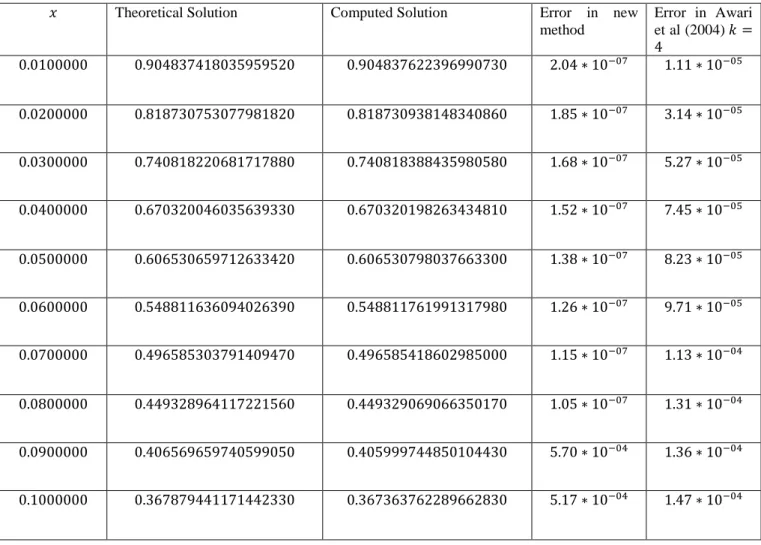
4.2. Example 2
𝑦′′− 100𝑦 = 0, 𝑦(0) = 1, 𝑦′(0) = −10, ℎ = 0.01
Exact Solution: 𝑦(𝑥) = 𝑒−10𝑥
Table 2: Comparison of the new method with Awari et al. (2004) for solving Problem one
𝑥 Theoretical Solution Computed Solution Error in new
method
Error in Awari
et al (2004) 𝑘 =
4
0.0100000 0.904837418035959520 0.904837622396990730 2.04 ∗ 10−07 1.11 ∗ 10−05
0.0200000 0.818730753077981820 0.818730938148340860 1.85 ∗ 10−07 3.14 ∗ 10−05
0.0300000 0.740818220681717880 0.740818388435980580 1.68 ∗ 10−07 5.27 ∗ 10−05
0.0400000 0.670320046035639330 0.670320198263434810 1.52 ∗ 10−07 7.45 ∗ 10−05
0.0500000 0.606530659712633420 0.606530798037663300 1.38 ∗ 10−07 8.23 ∗ 10−05
0.0600000 0.548811636094026390 0.548811761991317980 1.26 ∗ 10−07 9.71 ∗ 10−05
0.0700000 0.496585303791409470 0.496585418602985000 1.15 ∗ 10−07 1.13 ∗ 10−04
0.0800000 0.449328964117221560 0.449329069066350170 1.05 ∗ 10−07 1.31 ∗ 10−04
0.0900000 0.406569659740599050 0.405999744850104430 5.70 ∗ 10−04 1.36 ∗ 10−04
0.1000000 0.367879441171442330 0.367363762289662830 5.17 ∗ 10−04 1.47 ∗ 10−04
5. Conclusion
It is observed from Table 1 that the result obtained from the method is more efficient when compared to that of Badmus and Yahaya (2009). However, even though the error in the Block method proposed by Badmus and Yahaya (2009) seemed to
have produced a good result at it points of evaluation, it should be noticed that the method had step number 𝑘 = 5 against
our method with step number 𝑘 = 2.
Also, in Table 2, it is also observed that the error in Awari et al (2004) also seemed to have a good result at its points of
evaluation. It should also be noticed that the method in Awari et al (2004) had step number 𝑘 = 4 against our method with
step number 𝑘 = 2.
All computations were carried out using MATLAB 2008 and executed on Windows8 operating system.
34
[1]. S.O. Fatunla, Block methods for second order IVPs. International Journal of
Computer Mathematics, 42(9), (1991), 55-63.
[2]. S.O. Fatunla, Block methods for second order initial value problems. International Journal of Computer
Mathematics, 41, (1994), 55-63.
[3]. D.O. Awoyemi, A class of continuous Stormer-Cowell type methods for special
second order ordinary differential equations. Spectrum Journal, 5(1 & 2), (1998),100-108.
[4]. Z.B. Omar, & M.B. Suleiman, solving second order ODEs directly using parallel 2-point explicit block method.
Prosiding Kolokium Kebangsaan Pengintegrasian Teknologi Dalam Sains Matematik, Universiti Sains Malaysia, (1999), 390-395
[5]. P. Onumanyi, U.W. Sinsena, & Y. Dauda, Toward uniformly accurate continuous finite difference approximation
of ordinary differential equations. Bagale Journal of Pure and Applied Science, 1(2001), 5-8.
[6]. T.E. Simos, Dissipative trigonometrically-fitted methods for second order IVPs with oscillating solutions. Int. J.
Mod. Phys, (2002), 13(10), 1333-1345.
[7]. Z. Omar, & M. Suleiman, Parallel R-point implicit block method for solving higher order ordinary differential
equation directly. Journal of ICT., (2003), 3(1), 53-66.
[8]. Y.S. Awari & AA. Abada, A class of seven-point zero stable continuous block method for solution of second order
ordinary differential equation. International Journal of Mathematics and Statistics Invention (IJMSI), 2(2014),
47-54
[9]. Y. Yusuph, & P. Onumanyi, New Multiple FDMs through Multistep Collocation for 𝑦′′ = 𝑓(𝑥; 𝑦). In: Proceedings
of the Conference Organized by the National Mathematical Center, Abuja, Nigeria. (2005)
[10]. S.O. Adee et al, Note on starting the Nemerov method more accurately by a
hybrid formula of order four for an initial—value problem. Journal of Computational and Applied Mathematics,
175(2005) 369–373
[11]. Z.B. Omar, & M.B. Suleiman, Solving Higher Order ODEs Directly Using Parallel 2-point Explicit Block Method.
Matematika, (2005), 21(1), 15-23.
[12]. Z.A. Majid, M.B. Suleiman & Z. Omar, 3-point implicit block method for solving ordinary differential equations.
Bulletin of the Malaysian Mathematical Sciences Society (2006), (2), 29(1), 23-31.
[13]. Z.A. Majid & M.B. Suleiman, Two-point block direct integration implicit variable step method for solving higher
order systems of ordinary differential equations. In: Proceedings of the World Congress on Engineering II, (2007),
812-815.
[14]. S.N. Jator, A sixth order linear multistep method for the direct solution of
𝑦′′ = 𝑓(𝑥, 𝑦, 𝑦′). International Journal of Pure and Applied Mathematics, (2007), 40(4), 457-472.
[15]. A.O. Adesanya, T.A. Anake, & M.O. Udoh, Improved continuous method for
direct solution of general second order ordinary differential equations. Journal of Nigerian Association of
Mathematical Physics, 13(2008), 59-62.
[16]. A.O. Adesanya, T.A. Anake, & G.J. Oghoyon, Continuous implicit method for the solution of general second order
ordinary differential equations. Journal of Nigerian Association of Mathematical Physics, 15(2009), 71-78.
[17]. A.M. Badmus, & Y.A. Yahaya, An accurate uniform order 6 block method for direct solution of general second
order ordinary differential equations. Pacific Journal of Science and Technology, (2009), 10(2), 248-254.
[18]. Z.A. Majid, N.A. Azimi, & M. Suleiman, Solving second order ordinary
differential equations using two-point four step direct implicit block method. European Journal of Scientific
Research, (2009), 31(1), 29-36.
[19]. Z.B. Ibrahim, M. Suleiman & K.I. Othman, Direct block backward differentiation formulas for solving second order
ordinary differential equations. (2009).
[20]. S.N. Jator, & J. Li, A self-starting linear multistep method for a direct solution of the general second-order initial
value problem. International Journal of Computer Mathematics, (2009), 86(5), 827-836.
[21]. T. A. Anake, D. O. Awoyemi and A. A. Adesanya, One-step implicit hybrid block method for the direct solution of
general second order ordinary differential equations, IAENG International Journal of Applied Mathematics, 42
(2012), no. 4, 224-228.
[22]. T. A. Anake, D. O. Awoyemi and A. A. Adesanya, A one step method for the solution of general second order
ordinary differential equations, International Journal of Science and Technology, 2 (2012), no. 4, 159- 163.
[23]. D. O. Awoyemi, E. A. Adebile, A. O. Adesanya and T. A. Anake, Modified block method for the direct solution of
Akeremale et al.