Thesis Final .pdf

1

SHOULD REIT INVESTORS CARE ABOUT CASH FLOW

VARIABILITY?

By

Zicheng Ye

Senior Honors Thesis

Department of Economics

University of North Carolina at Chapel Hill

April 2018

Approved:

2

Acknowledge

I would like to sincerely thank my thesis advisor Dr. Michael Aguilar for his

endless patience, guidance and contributions to this honors thesis project. Dr.

Aguilar has been constantly encouraging me to think in an open-ended way,

which would be beneficial not only for my academics but also for my whole life.

I would also like to thank Dr. Lutz Hendricks for hosting the class and providing

constructive advice on my project throughout the semester. Finally, I would like

to thank all my classmates for the peer reviews and discussions, and the

3

Abstract

In this study, we ask whether firms with differing cash flow variability have different impacts

upon the benefits to portfolio diversification. We focus our attention on REITs since they offer

a unique venue to gauge the importance of cash flow variability, and we judge benefits to

diversification through a utility framework predicated upon Boudry et al. Using data from 2011

through 2017, we find three main results. First, the relation between cash flow variations and

portfolio diversification benefits exists but are not robust across different cash flow measures

and choices for diversification benefits. Second, risk-averse investors favor REITs with higher

or lower cash flow variations more than REITs with medium cash flow variations. Finally,

some subsets of REITs provide additional information to cash flow variations and

4

1. Introduction

In this study we ask how do firm-level cash flows impact the investors. The Gordon Growth

Model (Campbell and Shiller 1988) shows importance of cash flow because it relates to the

current asset price. However, the volatility of the cash flow is of equal importance. Agency

cost hypothesis mentioned in Bradley (1998) believes firms with volatile cash flows will on

average pay out a greater proportion of their cash flows in the form of a dividend and therefore

provide benefits to investors, while Corporate Risk Theory (Minton 1999) suggests

shareholders are better off if a firm maintains stable cash flows, as cash flow volatility affects a

firm’s investment policy by increasing the costs of raising external capital and therefore firms

with smoother cash flows should be valued higher. Both theories connect firm-level cash flow

variability with asset valuation and return.

Frahm and Wiechers (2011), however, indicated that when holding a portfolio of assets, it is

the diversification effect among the different assets, not the individual asset return-risk pattern

that seems to contribute to a better portfolio performance. The rationale behind it is a portfolio

composed of different kinds of investments will yield higher returns and meanwhile pose a

lower risk level than any of its individual portfolio components do. Boudry et al (2014) uses

the wealth compensation ratio built from a utility framework to suggest one single dimension

of an asset is insufficient to evaluate the benefits from adding it to or removing it from a

portfolio. Therefore, in this paper, we examine if there is a connection between an asset’s

5

would help understand the information carried by cash flow variability in making asset

allocation under uncertainty.

In our study, we focus on investors allocating their funds across REITs, whose operating

features making them a suitable investment vehicle for addressing our main question of

interest. A unique feature for REIT industry is that by law a REIT company is required to

distribute at least 90% of their taxable income to shareholders annually in the form of

dividends. Thereby, REITs pass along almost all of their earnings to investors, suggesting that

company earnings and cash flows are better proxies for investor earnings. The high distribution

means less retained earnings. If the retained earnings are high, then it would be hard to

connecting cash flow with investor benefits. Moreover, REIT’s income and cash flow are also

predictable because they are derived from the rents paid to the owners of commercial

properties whose tenants sign leases for fix periods of time. Therefore, higher cash flow

variability could potentially signal an uncertainty in the lease contracts and other normal

operating activities.

Boudry (2015) assessed the diversification benefits of equity REITs by splitting them into

common stocks and preferred stocks. Different from Boudry, we will instead look at equity

REITs by their underlying property types because property type is a natural classification for

investors. Like real assets, equity REITs is classified by property type. National Association of

REIT categorizes REITs into 12 sectors, including Office REITs, Industrial REITs, Retail

REITs, Lodging REITs, Residential REITs, Timberland REITs, Healthcare REITs,

6

provides information to the premiums or discounts from net asset value (Capozza 1995), a

REIT valuation metric. Moreover, property type is a natural proxy for cash flow variability, as

REITs derive revenue from their rental income and their leases are structured differently

depending on the property type. Table 1.0 below provided by BofAML REIT report displays

the average leasing length for each property type. The report also suggests that longer lease

terms under a locked lease rate generally provide greater income visibility and hence suggest

less cash flow variation.

Hotel Storage Residential Retail Industrial Office Healthcare

Daily Monthly 6-12 months 3-5 or 15-20 years (Triple net lease1)

6 years 5-7 years 10-20 years

Table 1.0 Average Leasing Length by REIT Property Type

The remaining parts of the paper are organized as follows: Section 2 reviews the relevant

literature on cash flow variability for asset pricing and the measures of portfolio diversification

benefits. Section 3 presents our data, followed by the detailed methodology and results in

Section 4. Section 5 conducts a robustness check and Section 6 provides our conclusions.

2. Literature Review

2.1 The use of cash flow and cash flow variability in asset pricing

Using cash flow as an informative content for stock return and asset pricing is not uncommon.

Though whether cash flow is the best estimator for asset valuation has been doubted in Liu

(2007), it has still been utilized as one important valuation metric. Rountree (2005) found a

7

negative relation between cash flow volatility and firm’s performance, measured by Tobin’s q,

whose positive relation with the average subsequent stock return was shown later in Ian

(2012); Da (2009) shows the change in the expected cash flow partly drives the cross-sectional

variation in stock returns. Inspired by the earlier dynamic Gordon Growth model (Shiller 1998),

Boudry (2015) found cash flow informative in pricing CMBS2 and suggested that it can be

applied to other types of thinly traded assets, including commercial real estate.

Our study builds on literature precedents and address whether the variability of cash flow is

equally important. Minton (1999) suggests shareholders are better off if a firm maintains

smooth cash flows. Rountree (2005) extends it and suggests smooth financials should be

valued higher. His findings indicate that investors value firms with smooth cash flows at a

premium relative to firms with more volatile cash flows and the magnitude of the effect is

substantial with one standard deviation increase in cash flow volatility resulting in

approximately a 32% decrease in firm value. In contrast with the traditional stock market,

whose cash flow payout ratio are inconsistent across industries, REITs have to distribute a

fixed percentage of their taxable income to shareholders, making the cash flow information

more valuable. Bradley (1998) connects future REITs cash flow uncertainty with the dividend

policy, which signals stock return. His regression model follows as: 𝑅_!−𝑅_!!= 𝑎+

𝑏 𝑅_!!"−𝑅_!! +𝑐𝐷!+𝑑∆𝐷!+𝑒𝐼!, with 𝑅! and 𝑅!!representing stock return and risk-free

return, whereas the dividend 𝐷!equals to 𝑓+𝑔𝐸!𝑌!!!+ℎ𝐸!𝜎! and 𝐸!𝜎! represents

anticipated volatility of cash flow available to shareholders. He concluded the variation in the

8

cash flow provides a negative signal to the stock return premium and is therefore inconsistent

with the agency cost theories.

In our research, we would incorporate Bradley’s dividend policy and EPS as the proxies for

REIT cash flow and cash flow variation. Using EPS and DPS also provides an insight whether

we can apply the same method to non-REIT industries. The Corporate Risk Theory (Minton

1999) uses operating cash flow (OCF) as the cash flow variable. However, for REITs,

traditional valuation metrics like book-market ratio and operating cash flow does not perfectly

apply for REITs because GAAP3 deducts depreciation and amortization factors, which are

important for real estate assets, from net income. Prior literatures focused on FFO4, funds from

operation, as a proxy for REIT cash flow. The unique industry specifics of REITs, like FFO

(funds from operations) and FAD5 (funds available for distribution), are typically utilized for

REIT valuation and to represent the cash flow, which provides better clues about how safe the

dividend is. Vincent (1999) noted that both FFO and EPS provide insight in REIT asset

pricing, with FFO better for management compensation and EPS better for financial reporting.

He also pointed out that FFO is not computed consistently across REITs because it is

self-reported. Bradley (1998) and Graham (2000) regarded FFO as a standard measurement for

REIT cash flow and found its significance over traditional GAAP measures like CFO6 and

EBITDA7 in REIT valuation. Therefore, we would focus on FFO as the main cash flow

variable in our research, and use DPS and EPS for robustness.

3 _{Generally Accepted Accounting Principle}

4 _{Net income minus gains from sales of property plus losses from sales of property plus impairment charges plus} real estate depreciation & amortization

5 _{An informal cash flow measure adjusting FFO for straight-line rents, leases and recurring real estate related} expenses. Unavailable for a majority of REITs.

6 _{Cash from Operations}

9

2.2 Portfolio Diversification and measure of diversification benefits

When hold a portfolio of assets, asset return itself becomes less informative since investors

need to consider the correlations among assets. Assessing the performance of a portfolio

therefore provide better information to investors. Bhuyan et al (2014) applies a mean-variance

utility function, and concludes REIT common stocks generate additional utility at low-medium

risk aversion levels. They used investor utility for assessing REIT benefits, and looked at the

risk premium and the correlation structure of the optimal portfolios containing REITs, stocks

and bonds. Boudry et al (2015) references an exponential utility framework and uses wealth

compensation ratio to estimate the diversification benefits of REIT common stocks and REIT

preferred stocks. Both precedents show that the return itself is insufficient to evaluate the

benefits for including a particular asset to a multi-asset portfolio. Therefore, we will look at the

portfolio diversification benefits of an asset instead of looking only at its return.

Literature precedents focus on the portfolio performance measures that provide risk-adjusted

return information for measuring portfolio diversification benefits8. The benefits to portfolio

diversification is the change in such measures when add or remove an asset, or a group of

assets, from a pre-specified portfolio based on investor’s objective functions. For example,

benefit can be captured by Wealth Compensation (Boudry 2015), which is the additional

wealth needed to compensate for the removal of a single asset to reach the initial level of utility

under a utility framework. The intuition is similar to the certainty equivalent of return, which is

the guaranteed amount of cash that yield the same expected utility as a given risky asset with

10

absolute certainty. In our research, we will use Boudry’s Wealth Compensation and the

traditional mean-variance Sharpe Ratio in order to include the portfolio risk-adjusted return

benefits. The detailed intuitions and mathematics of these measures will be covered in the

Section 4.

The contribution of our study to the asset pricing and portfolio diversification literature is that

we provide empirical evidence whether the firms of varying cash flow variations provide

benefits to portfolio diversification.

3. Data

The detailed monthly cash flow data are winnowed and extracted from IBES, NAREIT

REITWatch and REIT’s financial reports (10-K, annual report, quarterly report, etc.), including

Funds From Operations, Dividend Per Share and Earnings Per Share. Some REITs use

Adjusted FFO9 instead of FFO, and we will follow their IBES data and adjust accordingly.

NAREIT and SNL provide detailed lists of REIT companies by property type. Since REITs are

subject to structural change, we will have Hotel/Lodging, Self-Storage, Industrial, Retail,

Residential, Healthcare, Manufactured Homes, Office, Timberland and Diversified REITs10 as

the 10 property types11 for consistency. Table 1.1 looks at the average FFO and variation for

each property type indices from 2000 to 2017, assisted by Figure 0 provided by NAREIT

9_{AFFO: FFO with adjustments made for recurring capital expenditures used to maintain the quality of the REIT’s} underlying assets, generally equal to FFO.

11

Monthly Tracker. The coefficient of variation adjusts for the sample size dividing standard

deviation by mean, the difference in which shows the existence of FFO variation disparity by

property types. For the firm-level data, we select 98 REITs with complete cash flow data over

the last 7 years, and CRSP provides their historical price level. The reason for choosing 7 years

is REITs on average tends to have a short lifespan. Tables 2.1 in Appendix looks at our

selected 98 REITs at their firm levels. We would stick to the 98-REIT universe in the later

stages. Table 2.1 groups REITs by their property types and displays the descriptive statistics of

REIT return, cash flow and variation between March 2011 and September 2017. Note that the

FFO values for Timberland REITs are missing because they do not report their FFO. The

expected return and variation are converted to an annual basis. Due to the difference in the

sample size, the average expected return and cash flow are adjusted both across time and

across sector. For example, the average annual expected return, the average absolute FFO per

share, the average FFO per share variation for a single Office REIT over the last 7 years is

10.6%, 0.676 and 0.119 respectively. The variations in the cash flow are captured in FFOVar,

EPSVar and DPSVar. On average, Self-Storage REITs (23%, 0.251)12 have high average

expected return, FFO and DPS variation, while Retail (10%, 0.099) and Healthcare REITs

(13%, 0.097) tend to have more stable cash flow values with a lower average expected return.

The table results show the existence of difference in return and cash flow variation by property

type. We would use this grouping in the later regression analysis in Section 4.2. Table 2.2

below shows the descriptive data for our selected REITs from March 2011 to September 2017,

grouped by their cash flow variability. 5 REITs are deleted for FFO because of data

incompleteness.

12

Table 2.2 Descriptive Data for Cash flow Variation

Mean represents the average cash flow variations during the selected time horizon. FFO

displays a similar descriptive statistics to DPS. EPS shows a higher historical cash flow

variation. The difference in the descriptive statistics among cash flow proxies could potentially

leads to different results in our later analysis.

4. Methodology and Empirical Results

In the first part of methodology, we would show that the benefits to diversification vary for

investors with different risk aversions and for cash flow variations. We select a utility

framework as investor’s objective functions. The diversification benefit of a REIT group is the

Wealth Compensation after it is removed from the investable REIT universe. Second part of

the study links diversification benefits with the cash flow variation and examine the

relationship in a panel regression.

EPS Low Med High FFO Low Med High DPS Low Med High Mean 0.12 0.25 0.70 Mean 0.05 0.10 0.24 Mean 0.02 0.05 0.16

Std 0.04 0.04 0.43 Std 0.02 0.02 0.13 Std 0.01 0.01 0.09

Max 0.18 0.35 1.97 Max 0.07 0.14 0.68 Max 0.03 0.07 0.37

Min 0.04 0.18 0.35 Min 0.02 0.08 0.14 Min 0 0.03 0.08

13

4.1.1 Utility Framework

Consider a simple constrained two-asset portfolio problem with expected returns 𝜇1, 𝜇2,

standard deviations 𝜎1, 𝜎2, and their correlation 𝜌. Investors with a conventional negative

exponential utility of wealth 𝑈 (𝑊) =−𝑒!!!! seek to maximize the terminal wealth and hence

the utility, given an initial endowment equal to 1 by default.A_!> 0 is the risk aversion level for

investor 𝑖. An investor starts with initial wealth W0, and invest across 𝑖 assets with returns

jointly normally distributed. Assume fully invested, 𝑊!=𝑊!, investors seek to maximize

expected utility,

max E[U [(𝑊̃)]] = max −𝑒!!!(!!!!.!!!!!!)

w1+w2=W0

where 𝜇𝑝 and 𝜎𝑝 are the expected return and standard deviation of his portfolio. The equation

equality obtains because a linear combination of normally distributed variables is normally

distributed. 𝜎_!! _{denotes for the portfolio variance, computed by summing up weighted}

individual asset risk and covariance among all assets. The mathematical expression is

𝜎_!! _{= (𝑤}

!∗𝜎!)! !

! + (𝑤!∗𝑤!∗𝜌!,!∗𝜎! ∗𝜎!), 𝜌!,! denotes for the correlation of return

among all assets. We set the long-only investment constraint, 𝑤_! ≥0. For solving the

optimization, we simplify the portfolio variance to 𝜎_!! _{= 𝑤}!_{Σ𝑤, whereas Σ denotes for the}

covariance matrix, and reduce the original objective to

Max 𝑈 =µ_!−0.5 a_!σ_!!_,

because of the exponential property. Consider a two-asset case, we solve the optimization by

forming the Lagrangian and differentiating it with respect to 𝑤1 and 𝑤2. 𝜑 stands for the

14

𝐿 𝑤_!,𝑤_!,𝜆_!,𝜆_!,𝜑

= 1+𝜇_! 𝑤_!+ 1+𝜇_! 𝑤_!−1

2a! 𝑤!!σ!!+𝑤!!σ!!+2𝑤!𝑤!𝜌σ!σ! −𝜆! −𝑤!−0 −𝜆! −𝑤!−0 −𝜑(𝑤!+𝑤!−𝑊!)

The interior solutions to the problem, when 𝜆_!,𝜆_! = 0, are:

𝑤1 = !!!!!!!!!! !! !_!!!

!!!

!! !!!!!"!!!!!!!!

𝑤2 =!!!!!!!!!!! !! !_!!!

!!! !!!!!!!"!!!!!!!!

The general solution for the optimal weight vector, followed by the similar intuition and

computational method, is

𝑤

=

!

Σ

!!

_𝜇

₊

!!"!!!_!

Σ

1,

with the Lagrangian 𝐿(𝑤,𝜆) =𝑤′𝜇−_!!𝛼𝑤!_{Σ𝑤- 𝜆(1}!_𝑤−𝑤

!). Here, “1” represents a column

vector of 1s.

To assess the diversification benefits of different REIT assets to investors segmented by risk

aversion, we employ Boudry’s wealth compensation. The investor achieves derived utility of

wealth,

𝑉n(𝑊0) = 𝐸[𝑈(𝑊̃n)],

where 𝑛 denotes that investor had access to the asset set with 𝑛 assets. Vn denotes for the

derived utility for n-asset portfolio. We restrict the investor from investing in one REIT

15

now contains (𝑛−1) asset groups and the investor achieves derived utility of wealth under the

constrained set,

𝑉𝑛−1(𝑊0) = 𝐸[𝑈(𝑊̃n-1)].

Wealth compensation, Δ𝑊𝑘 is the additional wealth required when asset 𝑘 is removed from the

investment opportunity set to restore utility to the level achieved under the initial asset set, and

is the solution to the equation,

𝑉𝑛−1 (𝑊0+Δ𝑊𝑘) = 𝑉𝑛(𝑊0).

𝑊𝑘 is measured in terms of initial wealth. To evaluate the relative impact of different REIT

assets in the investment opportunity set, we compare wealth compensation of REITs grouped

by cash flow variation. A relative wealth compensation is taken for comparing the

diversification benefits across risk aversion by scaling the wealth compensation with its

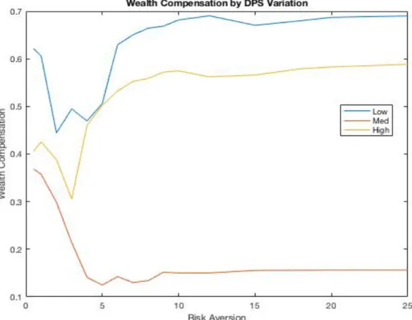
original wealth level. Figure 1.1 below, assisted with Table 4, presents the wealth

compensation at each selected risk aversion level for REITs grouped by their FFO variations.

The investment horizon is from March 2011 to September 2017, and we would use the average

cash flow variations from this period. “A” represents investor risk aversion level.

Low/Med/High represent the Wealth Compensation of the portfolio when REITs with

16

Figure 1.1 Wealth Compensation by REITs grouped by FFO Variation

The positions of the curves show the relative wealth compensation at each risk aversion level

for each REIT group. Higher position represents greater diversification benefit provided by this

REIT group because the removal of this group requires more wealth to restore the initial utility

level. The slope and trend of the curves along the x-axis show the change in the relative wealth

compensation for each group when risk aversion level changes. Upward sloping curve

indicates the diversification benefit of this REIT group increases when investors become more

17

A Low Med High 0.5 0.452 0.450 0.437 1 0.361 0.469 0.448 2 0.517 0.351 0.475 3 0.473 0.255 0.428 4 0.596 0.191 0.507 5 0.642 0.172 0.552 6 0.674 0.182 0.603 7 0.693 0.170 0.604 8 0.708 0.193 0.613 9 0.713 0.195 0.637 10 0.728 0.188 0.626 12 0.733 0.197 0.620 15 0.721 0.199 0.624 18 0.729 0.194 0.604 20 0.729 0.193 0.637 25 0.739 0.199 0.640

Table 3 Wealth Compensation, Grouped by FFO Variability

FFO variation shows a typical case for our observations: when risk aversion is low, REITs with

medium FFO variation posits at the top, representing its high benefits to diversification

because removing REITs with medium FFO variation requires more additional wealth to

compensate for the loss in utility than removing REITs with low or high FFO variation does.

The absolute effect is 46.9% of the original wealth for REITs with high FFO variation when

risk aversion level is 1. REITs with low FFO variation begins to get their roles at around risk

aversion level 2, the removal of which needs 16.6% (0.517-0.351) more wealth than REITs

with medium FFO does. The effect increases along with risk aversion indicated by the upward

sloping trend and the gap between two curves. When investors are highly risk averse at risk

18

compensation, more than triple of that for REITs with medium FFO variation (19.9%). Overall,

the FFO results show that investors would only choose REITs with medium and high FFO

variations when they are extremely risk loving. When investors are of mild and high risk

aversion, REITs with low FFO variability provides more diversification benefits, which

increases along with risk aversion level.

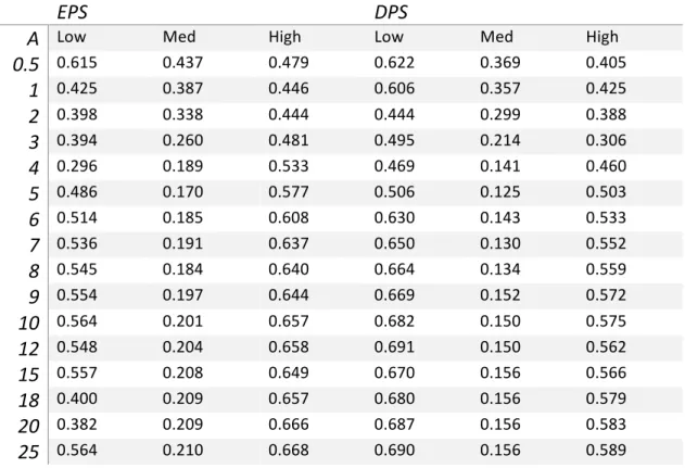
We display DPS and EPS results in Appendix Table 3 Cont. Both display the same trend across

risk aversion levels. When risk aversion increases, investors would less likely to invest in

REITs with medium cash flow variations because the removal of this group from their

portfolio requires fewer wealth to compensate for the loss in the expected utility than the other

two REIT groups do. DPS results are consistent with FFO results. Such heavy bias toward low

cash flow variation approximated by these two measures is consistent with what suggested in

the Corporate Risk Theory: firms with smoother cash flow should be highly valued.

Different from DPS and EPS, EPS results show that REITs with high EPS variation generates

higher benefits when investors are of high risk aversion. An explanation is REITs could

simultaneously have low average FFO and high average EPS variations during the selected

time horizon. We would break the whole investment horizon into subdivisions in the later stage

and see if the difference is caused by one single point measure of time.

4.1.3 Preliminary Conclusion

Our preliminary results show there exists a relation between the diversification benefits and

19

using FFO as the cash flow measure, our results show a negative relationship between FFO

variation and diversification benefits under a utility framework. Moreover, when investors

incorporate their risk aversion level into consideration, the more risk averse they are, the more

they would value REITs with cash flow variation at extreme ends higher, indicated by the

lower diversification benefits generated by REITs with medium cash flow variations.

4.2 Property Type Interaction

Since REITs are classified by their property types, whose leases are structured differently, the

variation of cash flow therefore could be significantly different among property types.

Knowing cash flow variation and property type interaction would help to determine if cash

flow variation as an indicator for investor benefits applies to all kind of REITs, or just a

subgroup of them. We note the commonalities in the cash flow variation and return by REIT

property types in Table 1 and Table 2.1 in Appendix. For example, Manufactured Home has

high historical return (21.6%) and FFO variation (0.12), which could signal the combination of

low FFO variation and Manufactured Homes provide potential return benefits to investors.

Same methods for finding the diversification benefits are applied to REITs grouped by

property types. Figure 2.1 and 2.2 illustrate the Wealth Compensation in relative to the original

wealth level across 6 risk aversion levels. In Figure 2.2, size effect13 _{is adjusted for each}

property type.

20

21

Figure 2.2 Relative Wealth Compensation by Property Type, Scaled by Sample Size

Clearly, the diversification benefits at REIT-level vary by property type and across risk

aversions. The trend of the curves shows the diversification benefits vary for different type of

investors classified by their risk aversion, and the position of the curves shows such benefit

varies by property type. After scaling for the sample size, Self-Storage and Manufactured

Home REITs14 on average provide the greatest diversification benefits, and their benefits

increase when risk aversion increases. When risk aversion is high, the removal of one

22

Manufacture Home REIT would on average require 21% of the initial wealth to compensate

for the loss in the expected utility. The removal of one Retail REIT at the same risk aversion

level would require only 2.5%, which means one Manufactured Homes REIT on average

provides diversification benefits approximately 8 times more than one Retail REIT does.

4.2.1 Cash Flow Variation Effect on Diversification Benefits, Exclude Property Type

We select one REIT property type at a specific risk aversion level, and use a 15-quarter rolling

window15 for assessing its average expected return and cash flow variation. We would then

compute for the diversification benefits of the selected REIT property type within that time

window and repeat for each time window and for each property type.

We first test the effect of cash flow variation on diversification benefits, independent of REIT

property type dummies. A significant positive coefficient on cash flow variation measures

would indicate REITs with high cash flow volatility provide more portfolio diversification

benefits, which echoes the Agency Cost Theory that favors high cash flow volatility. A

significant negative coefficient would indicate REITs with stable cash flow volatility provide

more portfolio diversification benefits, which follows the Corporate Risk Theory that smooth

cash flow generates higher investor benefits.

Our basic econometric model follows as

A: DBi,t = α0,i + α1* FFOi,t + α2* EPSi,t + α3* DPSi,t + εi,t

23

, whereas FFO , EPS and DPS capture the variation in FFO, EPS and DPS. DB is the Wealth

Compensation. We pick 5, 10 and 20 for representing low, medium and high investor risk

aversions under the utility framework.

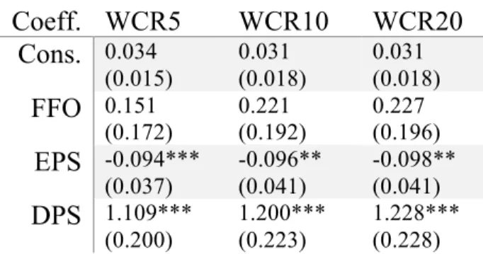
Table 6 below displays the results. WCR5, WCR10 and WCR20 represent the regression

results for cash flow variation on Wealth Compensation at risk 5,10 and 20. Wealth

Compensation shows a positive relation with FFO and DPS. When risk aversion level

increases, the effect of FFO increases from 0.151 to 0.227, which indicates that highly

risk-averse investors would love REITs with high FFO volatility more than risk-loving investors do

because the same 1-unit increase in the FFO variation would increase the wealth compensation

by 7.6% more for risk-averse investors. EPS shows a significant negative relation with Wealth

Compensation, and the effect turns more negative when risk aversion level increases. On

average, an increase in 1-unit EPS variation would reduce the Wealth Compensation by 0.096

units, and an increase in 1-unit DPS variation would increase the Wealth Compensation by 1.2

units. The rolling window sample method generates more accurate results opposite to the

relation reported in Section 4.1.2.

Coeff. WCR5 WCR10 WCR20

Cons. 0.034 (0.015)

0.031 (0.018)

0.031 (0.018)

FFO 0.151

(0.172) 0.221 (0.192) 0.227 (0.196)

EPS -0.094*** (0.037)

-0.096** (0.041)

-0.098** (0.041)

DPS 1.109*** (0.200) 1.200*** (0.223) 1.228*** (0.228)

24

4.2.2 Cash Flow Variation Effect on Diversification Benefits, Include Property Type

Our econometric model follows as

B: DBi,t = α0,i + α1* PTi,t +α2* FFOi,t +α3* DPSi,t +α4* EPSi,t + α5 * PTi FFOi,t + α6 * PTi

DPSi,t + α7 * PTi EPSi,t + εi,t

C: DBi,t = α0,i + α1* PTi,t +α2* CFVi,t + α3 * PTi CFVi,t + εi,t (Simplified)

, whereas DBi,t measures the diversification benefits of REIT property type i at time t, CFVi,t

represents the cash flow variability, captured by FFO, DPS or EPS variation, of REIT property

type i at time t. PTi stands for the 9 property type dummies (Hotel REIT, Residential REIT,

etc.). α1 measures the property type fixed effect in relative to the dropped property type

dummy. α2 represents the interaction effect between cash flow variation and the controlled

property type dummy. α3 measures the interaction effect between property types and their cash

flow variability, in relative to the interaction effect between the controlled property type

dummy and its cash flow variability. We interpret the sign and the significance level of α2 and

α3 to find whether property type adds information for cash flow variability in explaining

diversification benefits.

Table 7.1 shows an example of the linear fit results, with the first column recording the

interaction terms involved in the regression set up. The dropped property type is Manufactured

Homes, which means α2 captures the interactive effect between cash flow variation and the

Manufactured Homes dummy. The risk aversion level is 20. 1-unit increase in FFO variation

25

A 1-unit increase in FFO variation will increase the diversification benefit of Industrial REITs

4.15 units less than that of Manufactured Home REITs does, which means the interaction

effect, α2, between FFO and Industrial REITs is -2.24.

To capture the absolute, instead of the relative, interaction effect between cash flow variation

and every property type, we repeat the regression process by setting different controlled

property type dummies, and focus on the α2. Table 8 and Figure 3 below display the cash flow

interaction effect across property type at risk aversion level 20. Each entry in Table 8 denotes

for the interaction effect and its standard error. Each bar in Figure 3 represents the regression

coefficient for the cash flow variation and property type interaction effect. For example, the

lowest blue bar represents one unit increase in the FFO variation, given Industrial as the

property type, would decrease Wealth Compensation by 2.24 units. Table 8 Cont. in Appendix

contains the results for Wealth Compensation at risk aversion level 5.

Figure 3 Property Type Interactions on Wealth Compensation -3

-2 -1 0 1 2 3

DIV RESI OFF STOR RET HEAL HOT IND MH

Property Type Interaction on Wealth Compensation

FFO

26

WCR20 DIV RESI OFF STOR RET HEAL HOT IND MH

FFO 0.01 0.50 -0.02 0.18 0.58 0.60 0.10 -2.24*** 1.09***

(0.14) (0.36) (0.43) (0.75) (1.84) (0.72) (0.43) (0.58) (0.39)

EPS 0.05 0.04 0.08 0.47 0.02 0.02 -0.09 -0.30*** 0.04

(0.30) (0.04) (0.07) (0.70) (0.13) (0.13) (0.10) (0.11) (0.05)

DPS -1.28 -0.08 -0.05 0.16 -0.24 -0.24 -0.40 2.55*** -0.34***

(0.71) (1.28) (0.20) (0.36) (1.42) (1.42) (0.35) (0.62) (0.14)

Table 8. Property Type Interactions on Wealth Compensation, RA=20

Property type dummies tend to provide positive interaction effect on FFO and EPS, and

negative interaction effect on DPS. However, only Industrial and Manufactured Home provide

some significant results for Wealth Compensation. Based on these results and our observation

in Figure 2.2, we conclude the difference in diversification benefits by property type is not

completely due to their underlying cash flow variations, except for Manufactured Homes and

Industrial REITs, whose underlying cash flow variations contribute for their varying benefits to

diversification.

5. Robustness

For robustness check, we select a different framework and a different diversification benefit

measure, to see if the results follow those obtained under the utility framework. Our selected

objective function is the widely used Maximum Sharpe Ratio based on the mean-variance

framework, whose aim is to optimize portfolio Sharpe Ratio regardless of risk aversion, which

27

The change of the Sharpe Ratio captures the diversification benefit of the REIT subgroup we

are measuring. The MSR portfolio seeks to maximize the risk-adjusted return,

𝑀𝑎𝑥

[

]

−

𝑟𝑓

𝜎𝑝

, µ! = !!𝑤! ∗µ! is the portfolio return with 0≤ 𝑤! ≤ 1for the long-only constraint and

𝑤_! !

! =1 for the fully investment constraint. µ!represents the weight and average expected

return of asset i. 𝑟𝑓 is the risk-free rate, approximated by average 1-Month Treasury Bond

Yield over the sample period. Similarly, we will first find the MSR portfolio containing all

sample REITs, and the MSR portfolios after removing a REIT subgroup.

For solving the optimization, we form the Lagrangian, 𝐿 𝑤,𝜆 = (𝑤!_{𝜇−𝑟𝑓)(𝑤}!_Σ𝑤)!!_!+

𝜆(𝑤!_{1′−1), differentiate with respect to w and obtain the optimal solutions,}

𝑤 = Σ

!!_(𝜇−

_𝑟

₎

1!_Σ!!_(𝜇−

_{𝑟𝑓1′)}

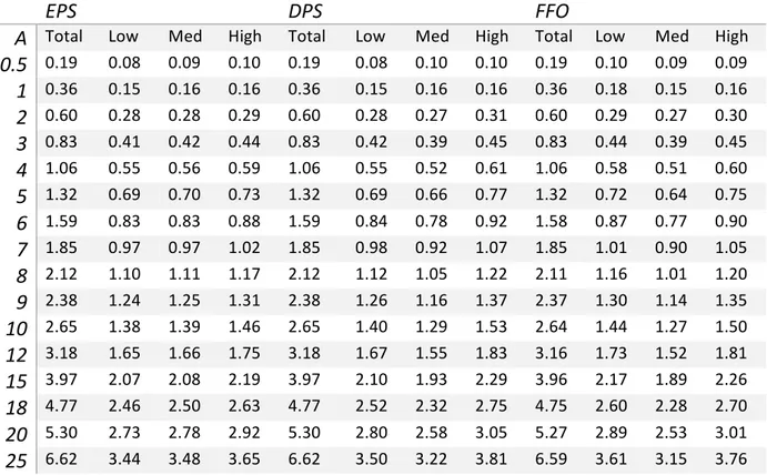
Table 4 displays the Maximum Sharpe Ratio for REITs grouped by cash flow variation.

“Total” represents for the n-asset portfolio Sharpe Ratio. “Low” represents for the portfolio

without REITs with low cash flow variations. We eliminated REITs with incomplete FFO data.

Therefore, the full-sample Sharpe Ratio is slightly lower than that of EPS and DPS grouped

portfolios. FFO case shows an opposite results to what we have obtained under the utility

framework. REITs with high FFO tend to provide more portfolio diversification benefits

indicated by the change of the Maximum Sharpe Ratio. 19.2% decrease in the Sharpe Ratio

28

EPS and DPS. Based on our MSR results, higher FFO and DPS variation leads to a higher

diversification benefits, which is consistent with the Agency Cost Theory: since REITs by law

have to distribute a higher amount of cash flows in the form of dividends, if they also have

higher cash flow volatility, the combination of which follows Bradley’s reasoning that firms

with volatile cash flow pays out higher dividend and therefore provide more benefits to

investors. We notice the difference in the results due to the weights assigned to different REITs

for two frameworks, because for the Wealth Compensation, the sum of individual weights is

W0 instead of 1 for the MSR setup. A small variation in weights would lead to a different

value in the diversification benefits.

CF TOTAL LOW MED HIGH

EPS 2.05 1.77 1.77 2.04

DPS 2.05 2.03 1.74 1.69

FFO 2.03 2.03 1.72 1.64

Table 4 Changes in MSR by REIT Cash Flow Variations

We repeat 4.2.1 and 4.2.2 for the MSR framework, and the results are reported in Table 6

Cont., Table 8 Cont. and Figure 3 Cont. in Appendix. 1-unit increase in the FFO variation

increases the Sharpe Ratio benefit by 0.111 units, significant at 0.001 level. 1-unit increase in

the EPS variation decreases the Sharpe Ratio benefits by 0.032 units, significant at 0.001 level.

The results are consistent with the regression results obtained under the utility framework, but

29

The property type interaction effect for the MSR case shows only Self-Storage provides

additional FFO and EPS interaction effect to the Sharpe Ratio benefit. 1-unit increase in the

FFO variation, given Self-Storage as the property type, increases Sharpe Ratio benefit by 2.2

units. Manufactured Home does provide additional DPS interaction effect, but inconsistent

with the utility framework results, Industrial REITs do not show any additional interaction

Sharpe Ratio benefits to portfolio diversification. We conclude investors would get benefit

paying attention to the cash flow variations of Manufactured Homes, Self-Storage and

Industrial REITs, but such property type interaction effect is not robust across measures for

diversification benefits.

6. Summary and Limitations

Our study looks at if the variation of cash flow provides information to the benefits to

diversification for investors allocating their funds across REIT property types. We focus our

attention on REITs because the industry required dividend payout policy and the different lease

structures by property types make REIT a useful universe to address our main question of

interest.

We conduct our analysis using REIT data spanning the period March 2011 to September 2017

and take 15-month as one sample rolling period. The 98 selected REITs satisfy two conditions:

they are alive during the selected period and they have full firm-level cash flow data. For

robustness, we use three cash flow measures, namely Funds From Operations, Earnings Per

30

Sharpe Ratio and Wealth Compensation. They both include more than one single dimension of

assets into consideration to measuring investor’s benefits. We use a utility framework to find

the Wealth Compensation and conduct a robustness check using the Maximum Sharpe Ratio

framework.

We establish three main results. First, there exists a relation between cash flow variations to

portfolio diversification benefits, but such relation depends on the selection of cash flow and

diversification benefit proxies: REITs with higher FFO variation tend to provide more benefits

to portfolio wealth and High EPS variation does harm to it. Such relation is robust across

different measures of diversification benefit. The difference in the direction of effects provides

insight on cash flow variation: both Corporate Risk Theory and Agency Cost Theory result in

one-sided conclusions how cash flow variation would affect asset return, but perhaps it is due

to the selection of cash flow variation and objective measures that divaricate the theoretical

results.

Secondly, investors segmented by risk aversion levels would treat cash flow variation with

different views. The absolute effect of cash flow variations and REIT property type

interactions tend to increase along with the risk aversion, which implies investors are more

cautious to cash flow variation data when they become more risk averse. Our results also

implies risk-averse investors would prefer REITs with high FFO and DPS variation and low

EPS variation more than risk-loving investors do, shown by the increase in the absolute value

of the regression coefficient across regression models. Finally, we notice Manufactured

31

flow variation and hence the diversification benefits. The effects are robust for across cash

flow measures, but are not robust across diversification benefit measures.

The limitation of our research lies in the selection of benefits to diversification and the sample

size. Literature records benefits to diversifications in different ways, and we pick the Wealth

Compensation and Sharpe Ratio because they compute for both return and risk information of

a portfolio, which would be beneficial for investors. However, the different computation

constraints and method for the Wealth Compensation and the Sharpe Ratio would lead to

completely different results, since by nature the Wealth Compensation is a dollar amount

measured in terms of investor’s initial wealth, while Sharpe Ratio provides risk-adjusted return

information of a portfolio. Moreover, our sample only includes 101 REITs16 that are alive over

our full sample period due to the short average REIT lifespan. We eliminate REITs with

undefined property types and with changing property types for creating a balance panel for the

regression, but the small sample size yields higher standard error terms, and also affects the

optimization results under the Maximum Sharpe Ratio framework, which is possibly to output

ended solution that assigns 100% of weight on a single asset either because of its superior

expected return or its small variance. More assets would allow a more valuable covariance

matrix, and hence a better estimation for the diversification benefits. Appendix includes

another measure of portfolio diversification, Diversification Ratio, which solely focuses on the

covariance structure and hence the risk component of the portfolio. An extension of this

research could test cash flow variations on the variant measures for diversification benefits.

32

Appendix

There is no canonical way to quantitatively define portfolio diversification. In the main text we

focus on Wealth Compensation and Sharpe Ratio that provide risk-adjusted return information

for the portfolio and include more than one single dimension of assets. Another class defines

effective diversification as “not heavily expose to one single asset,” (Woerheide 1993) and

focuses exclusively on the number of assets in a portfolio or the portfolio variance-covariance

structure. The quantitative measures from this class include Portfolio Herfindahl Index,

Rosenbluth Index, Portfolio Diversification Index (Rubin 2006), Diversification Distribution

(Meucci 2009), Diversification Ratio (Choueifaty 2008) and Non-Avoidable Return Variation

(Frahm 2011), which measure the degree individual asset risk has been ruled out by the

portfolio covariance structure.

In our research, we also selected the Diversification Ratio (Choueifaty 2008) as a portfolio

diversification measure and repeated Section 4 based on it. The reasoning for including such

portfolio diversification measure and results we obtained are reported below.

Compare with Portfolio Herfindahl Index and Rosenbluth Index that solely focuses on

portfolio weights, Diversification Ratio incorporates asset risks and the correlation structures,

the computation of which considers more than one single dimension of an asset. Compare with

Portfolio Diversification Index and other multi-dimensional measures, Diversification Portfolio

can be applied to a wider range of portfolios17 (Choueifaty 2008). Choueifaty and Coignard

define the Diversification Ratio as the ratio of the weighted average of volatilities divided by

33

the overall portfolio volatility. Except for the mono-asset and independence case, the

diversification ratio will be strictly higher than 1 under the long only condition. The

Diversification Ratio embodies the nature of portfolio diversification: the risk of the

combination of assets should be lower than the combination of the risks. A portfolio with a

high Diversification Ratio is built without using any speculative marketplace views regarding

the future risk compensation of the constituent stocks. However, holding more assets does not

necessarily increase a portfolio’s Diversification Ratio because of a potentially poorer

correlation structure.

We look at the portfolio variance-covariance structure by referencing the Diversification Ratio

𝐷𝑅 𝑝 = !!!"∗!" !"

with 𝜔𝑖 the optimal weight for asset i. The optimal weights are the weights assigned to

individual assets derived from maximizing investor’s objective function. DR looks at the

co-movement across assets, and it is unbounded from above, with higher values reflecting the

diversifying effects of relatively low correlation across assets because a higher DR essentially

means the combination of the risks exceeds the risk of the combination of assets. With the

long-only constraint, DR bounds below by 1. That is when only one asset is assigned weight or

assets are perfectly uncorrelated.

The figure below shows the Diversification Ratio by FFO variation across risk aversions.

34

aversion, which is inconsistent with the results obtained from both Wealth Compensation and

Sharpe Ratio.

Figure FFO Variation on Diversification Ratio

Our regression results using Diversification Ratio as a portfolio diversification measure leads

to a similar cash flow-diversification benefit results as Wealth Compensation does. DPS and

EPS variation show significant relations to benefits to diversification. Detailed statistics are

35

Reference

BofAML REITs Research, “BofAML REIT primer, 6th ed”. Bank of America Merrill Lynch. Industry Handbook.

Boudry Walter, Crocker Liu, Tobias Muhlhofer, Torous Walter (2015). “Using Cash Flow Dynamics to Price Thinly Traded Assets.” Cornell School of Hotel Administration Collection, Working Papers

Boudry Walter, deRoos Jan, Ukhov Andrey (2015). Diversification Benefits of REIT Preferred and Common Stock: New Evidence from a Utility based Framework. 2015 NAREIT/AREUEA Real Estate Research Conference

Bradley Michael, Capozza Dennis, Seguin Paul (1998). “Dividend Policy and Cash-Flow Uncertainty.” Real Estate Economics, Volume 26, Page 555-580

Campbell J. Y. and Shiller, R. J. (1988a). “The dividend price ratio and expectations of future dividends and discount factors”. The Review of Financial Studies 1(3), 195–228.

Campbell J. Y. and Shiller, R. J. (1988b). “Stock prices, earnings and expected dividends”. Journal of Finance 43(3), 661–676.

Capozza Dennis, Lee Sohan (1995). Property Tyep, Size, and REIT Value. Journal of Real Estate Research. 10. 363-380.

Choueifaty Yves, Coignard Yves (2008). “Toward Maximum Diversification.” The Journal of Portfolio Management. Vol.35, Issue 1.

DeMiguel, Victor, Lorenzo Garlappi, and Raman Uppal (2009), “Optimal versus naive diversification: How inefficient is the 1/N portfolio strategy?” The Review of Financial Studies 22 (5), 1915–1953

Frahm Gabriel, Wiechers Chrisof (2011). “On the Diversification of Portfolios of Risky Assets.” University of Cologne, Seminar of Economic and Social Statistics, Working Papers

Graham Carol, Knight John (2000). “Cash Flows vs. Earnings in the Valuation of Equity REITs.” The Journal of Real Estate Portfolio Management, Vol.6, No.1, Page 17-25

Kuhle James (1978) “Portfolio Diversification and Return Benefits--- Common Stock vs. Real Estate Investment Trusts (REITs).” The Journal of Real Estate Research, Vol.2, Issue 2, Page 1-9.

Kuhle James, Bhuyan Rafiqul, Ikromov Nuriddin, Chiemeke Charles (2014). Optimal Portfolio Allocation among REITs, Stocks, and Long-Term Bonds: An Empirical Analysis of US

Financial Markets. Journal of Mathematical Finance 04. 104-112.

Liu Jing, Nissim Doron, Thomas Jacob (2007). “Is Cash Flow King in Valuations?” Financial Analysts Journal, Vol.63, No.2

36

Minton, B., and Schrand, C. (1999). “The Impact of Cash Flow Volatility on Discretionary Investment and the Costs of Debt and Equity Financing.” Journal of Financial Economics 54, 423-460.

Purnanandam (2007). “Financial distress and corporate risk management: Theory and evidence”

Rountree Brian, Allayannis George, Weston James (2005). “Earning Volatility, Cash Flow Volatility, and Firm Value”

Rudin Alexander M., Jonathan S. Morgan (2006). “A portfolio diversification index,” The Journal of Portfolio Management, 32(2), Page 81–89.

Vincent Linda (1999). “The information content of funds from operations (FFO) for real estate investment trusts (REITs).” Journal of Accounting and Economics, Volume 69, Page 104

Woerheide Walt, Persson Don (1993). “An Index of Portfolio Diversification.” Financial Services Review 2(2), Page 73-85

37

Table 1 17-year average Funds from Operation, by REIT property type, in Millions Table shows the descriptive statistics for the FFO by REIT property type from 2000 to 2017.

The first row represents the average FFO and the second row represents the standard deviation of the FFO over 17 years. The standard deviation is also the FFO variation. The third row adjusts for the FFO variation by dividing its mean.

OFF IND RET RESI MANU DIV HOT STOR HEAL

Mean 1034.8 500.7 1833.6 948.8 63.1 480.4 505.5 346.6 672.4

SD 304.4 280.8 757.3 338.5 40.4 290.9 371.56 157.18 509.03

38

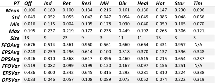
Table 2.1 Expected Return and Cash Flow Variation by Property Type, 2011-2017, 98 REITs

Table reports the average expected annual return, standard deviation, size and cash flow variation of the selected 98-REITs grouped by property type. FFOAvg, EPSAvg and DPSAvg represent the average absolute FFO, EPS and DPS value per REIT under each property type. FFOVar, EPSVar, DPSVar represent the standard deviation of FFO, EPS and DPS, which are equal to our cash flow variability. All reported data are adjusted by sample size under each property type and is on per-REIT level.

PT Off Ind Ret Resi MH Div Heal Hot Stor Tim Mean 0.106 0.189 0.100 0.134 0.216 0.161 0.130 0.147 0.230 0.096

Std 0.049 0.052 0.055 0.042 0.047 0.054 0.049 0.086 0.048 0.056 Min 0.016 0.115 0.004 0.105 0.178 0.030 0.040 0.059 0.165 0.070 Max 0.195 0.237 0.219 0.172 0.235 0.449 0.192 0.265 0.306 0.121

Size 13 9 23 9 3 11 11 13 3 3 FFOAvg 0.676 0.514 0.561 0.960 0.561 0.660 0.664 0.431 0.957 N/A

EPSAvg 0.248 0.259 0.296 0.614 0.100 0.318 0.370 0.137 0.596 0.348 DPSAvg 0.326 0.310 0.368 0.617 0.396 0.460 0.515 0.215 0.654 0.237 FFOVar 0.119 0.082 0.099 0.199 0.120 0.167 0.097 0.156 0.251 N/A

39

Table 3 Cont. Wealth Compensation, Grouped by Cash Flow Variability

Table shows the wealth levels of REIT portfolios derived from Boudry’s utility framework, long-only condition. The change in the wealth level is the Wealth Compensation. REITs are grouped by their cash flow variability. The first 4 columns reports the DPS case, the last 4 columns reports the EPS case. “A” represents investor risk aversion level. At high risk aversion, investors would have negative wealth. Low/Med/High represent the Wealth Compensation of the portfolio when REITs with low/medium/high cash flow variations are removed.

EPS DPS

A Low Med High Low Med High

40

Table 5 Diversification Ratio, Grouped by cash flow variation

Table shows the Diversification Ratios of REIT portfolios derived from Boudry’s utility framework, long-only condition. A represents investor risk aversion level. REITs are grouped by their cash flow variability. The first 4 columns show the result for DPS variation as a proxy for cash flow variation. The mid 4 columns show the result for FFO variation. The right 4 columns show the result for EPS variations. Low/Med/High represent the Diversification Ratio of the portfolio when REITs with low/medium/high cash flow variations are removed.

EPS DPS FFO

41

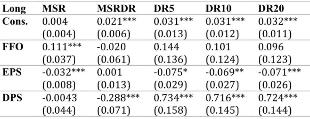
Table 6 Cont. Diversification Benefit by Cash Flow Variation

Table displays the result for the regression DBi,t = α0,i + α1* FFOi,t + α2* EPSi,t + α3* DPSi,t +

εi,t with the long-only constraint. Each entry displays the estimate and the standard deviation

terms. *** stands for significant at 0.01. ** stands for significant at 0.05. * stands for significant at 0.1. The first column includes FFO, EPS, DPS and the intercept as four x-variables. The first row specifies the y-variable used. MSR represents the Maximum Sharpe Ratio derived from the MSR framework. MSRDR represents the Diversification Ratio derived from the MSR framework. MSR is for robustness check. DR5, DR10 and DR20 represent the Diversification Ratio, derived from Boudry’s utility framework, at risk aversion level 5, 10 and 20.

Long MSR MSRDR DR5 DR10 DR20

Cons. 0.004

(0.004) 0.021*** (0.006) 0.031*** (0.013) 0.031*** (0.012) 0.032*** (0.011) FFO 0.111***

(0.037) -0.020 (0.061) 0.144 (0.136) 0.101 (0.124) 0.096 (0.123) EPS -0.032***

(0.008) 0.001 (0.013) -0.075* (0.029) -0.069** (0.027) -0.071*** (0.026) DPS -0.0043

42

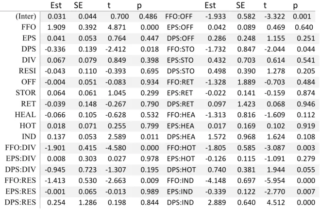
Table

Table displays the results of the regression DBi,t = α0,i + α1* PTi,t +α2* FFOi,t +α3* DPSi,t +α4* EPSi,t + α5 * PTi FFOi,t + α6 * PTi DPSi,t + α7 * PTi EPSi,t + εi,t. . Each entry displays the estimate and the standard deviation terms. *** stands for significant at 0.01. ** stands for significant at 0.05. * stands for significant at 0.1. Table only includes all cash flow variation and property type interaction terms. The dropped property type dummy is Manufactured Homes. Est. represents the regression coefficients. SE is the standard error. “t” stands for t-stats and p is the p-value.

Est SE t p Est SE t p

43

Table 8 Cont. Cash Flow Variation and Property Type Interaction Effects on Diversification Benefits

Table reports the interaction effects between property type and cash flow variation on diversification benefits, under the utility framework with no investment constraints. Each entry reports the estimate and standard deviation of the interaction effect. Property types from left to right are Diversified, Residential, Office, Self-Storage, Retail, Healthcare, Hotel, Industrial and Manufactured Homes. The first panel captures the long-only Wealth Compensation case when risk aversion is 5. The second panel captures the MSR case. The third panel captures the long-only Diversification Ratio case when risk aversion is 20.

WCR5 DIV RESI OFF STOR RET HEAL HOT IND MH

FFO -0.09 0.46 0.10 -1.47* 0.08 0.69 0.19 -2.11*** 0.75*

(0.14) (0.37) (0.45) (0.78) (1.91) (0.74) (0.45) (0.60) (0.41)

EPS -0.15 0.01 0.05 0.81 -0.03 -0.06 -0.11 -0.39*** 0.05

(0.31) (0.04) (0.07) (0.73) (0.13) (0.17) (0.11) (0.11) (0.05)

DPS -0.92 -0.31 -0.23 0.30 -0.29 0.66 0.37 3.01*** -0.15

(0.73) (1.32) (0.21) (0.37) (1.46) (0.99) (0.37) (0.65) (0.14)

MSR MH IND HOT HEAL RET STOR RESI OFF DIV

FFO 0.17 0.25 0.07 0.05 0.01 2.20*** 0.00 0.00 0.19

(0.28) (0.41) (0.31) (0.51) (0.01) (0.54) (0.26) (0.31) (0.10)

EPS 0.01 -0.01 0.03 0.01 0.00 2.84*** 0.00 0.00 -0.10

(0.04) (0.08) (0.07) (0.12) (0.09) (0.50) (0.03) (0.05) (0.21)

DPS -0.23*** -0.17 0.24 0.05 -0.01 0.43 0 0.00 0.03

(0.10) (0.45) (0.25) (0.69) (1.02) (0.26) (0.92) (0.15) (0.51)

DR20 DIV RESI OFF STOR RET HEAL HOT IND MH

FFO 0.14 -0.14 0.11 4.11*** -0.14 -0.27 -0.07 0.32 0.02

(0.13) (0.43) (0.51) (0.90) (2.21) (0.85) (0.52) (0.69) (0.47)

EPS 0.02 -0.02 -0.03 -1.50* -0.01 0.04 0.11 0.02 0.13**

(0.02) (0.04) (0.08) (0.84) (0.16) (0.19) (0.12) (0.13) (0.06)

DPS -0.04 -1.66 0.23 -0.90** -0.19 0.71 -0.21 0.07 0.06

44

Figure 0

Figure depicts the cumulative FFO by property types over the last 17 years. The

vertical axis has the unit in Millions. Data is provided by NAREIT Monthly

REIT Tracker.

-1,000.00 -500.00 0.00 500.00 1,000.00 1,500.00 2,000.00 2,500.00 3,000.00 3,500.00

2000.1 2000.3 2001.1 2001.3 2002.1 2002.3 2003.1 2003.3 2004.1 2004.3 2005.1 2005.3 2006.1 2006.3 2007.1 2007.3 2008.1 2008.3 2009.1 2009.3 2010.1 2010.3 2011.1 2011.3 2012.1 2012.3 2013.1 2013.3 2014.1 2014.3 2015.1 2015.3 2016.1 2016.3 2017.1

FFO by REIT Property Type from 2000 to 2017

Office Industrial Retail

45

Figure 1.1 Cont.

46

Figure 1.1 Cont.

47

Figure 1.2 Cont.

Figure illustrates the change in the Diversification Ratio by removing REITs with

EPS variations across risk aversions. The vertical axis represents the change in

the Diversification Ratio. The horizontal axis represents the risk aversion levels.

The yellow line represents the Diversification Ratio change after removing

REITs with high DPS variability. The red line is for removing REITs with

medium cash flow variability and the blue line is for removing REITs with cash

flow variability.

48

Figure 1.2 Cont.

49

Figure 3

Figure illustrates the interaction effect between property type and cash flow

variations on diversification benefit, approximated by Wealth Compensation

Ratio at risk aversion level 20. RA represents for risk aversion. The interaction

effects for each REIT property type are captured in the

terms from the

regression

-3 -2 -1 0 1 2 3

DIV RESI OFF STOR RET HEAL HOT IND MH

Property Type Interaction on Wealth Compensation, RA=20

FFO EPS

50

Figure 3 Cont.

Figure illustrates the interaction effect between property type and cash flow

variations on diversification benefit, approximated by Wealth Compensation

Ratio at risk aversion level 5. RA represents for risk aversion. The interaction

effects for each REIT property type are captured in the

terms from the

regression

-3 -2 -1 0 1 2 3 4

DIV RESI OFF STOR RET HEAL HOT IND MH

Property Type Interaction on Wealth Compensation, RA=5

FFO EPS

51

Figure 3 Cont.

Figure illustrates the interaction effect between property type and cash flow

variations on diversification benefit, approximated by Sharpe Ratio. RA

represents for risk aversion. The interaction effects for each REIT property type

are captured in the

terms from the regression

-4 -3 -2 -1 0 1 2 3

MH IND HOT HEAL RET STO OFF RESI DIV

Property Type Interaction Effect, MSR

FFO