2. NAIVE BAYES CLASSIFIERS

(1)

Spam Filtering with Naive Bayes – Which Naive Bayes?

∗

Vangelis Metsis

† Institute of Informatics and

Telecommunications, N.C.S.R. “Demokritos”, Athens, Greece

Ion Androutsopoulos

Department of Informatics, Athens University of Economics and Business,

Athens, Greece

Georgios Paliouras

Institute of Informatics and

Telecommunications, N.C.S.R. “Demokritos”,

Athens, Greece

ABSTRACT

Naive Bayes is very popular in commercial and open-source anti-spam e-mail filters. There are, however, several forms of Naive Bayes, something the anti-spam literature does not always acknowledge. We discuss five different versions of Naive Bayes, and compare them on six new, non-encoded datasets, that contain ham messages of particular Enron users and fresh spam messages. The new datasets, which we make publicly available, are more realistic than previous comparable benchmarks, because they maintain the tempo-ral order of the messages in the two categories, and they emulate the varying proportion of spam and ham messages that users receive over time. We adopt an experimental procedure that emulates the incremental training of person-alized spam filters, and we plotroccurves that allow us to compare the different versions of_nbover the entire tradeoff between true positives and true negatives.

1. INTRODUCTION

Although several machine learning algorithms have been employed in anti-spam e-mail filtering, including algorithms that are considered top-performers in text classification, like Boosting and Support Vector Machines (see, for example, [4, 6, 10, 16]), Naive Bayes (nb) classifiers currently appear to be particularly popular in commercial and open-source spam filters. This is probably due to their simplicity, which makes them easy to implement, their linear computational complexity, and their accuracy, which in spam filtering is comparable to that of more elaborate learning algorithms [2]. There are, however, several forms ofnbclassifiers, and the anti-spam literature does not always acknowledge this.

In their seminal papers on learning-based spam filters, Sahami et al. [21] used anb classifier with amulti-variate Bernoullimodel (this is also the model we had used in [1]), a form of_nbthat relies on Boolean attributes, whereas Pantel and Lin [19] in effect adopted themultinomial form of _nb, which normally takes into account term frequencies. Mc-Callum and Nigam [17] have shown experimentally that the ∗_{This version of the paper contains some minor corrections} in the description of Flexible Bayes, which were made after the conference.

†_{Work carried out mostly while at the Department of} Infor-matics, Athens University of Economics and Business.

CEAS 2006 - Third Conference on Email and Anti-Spam, July 27-28, 2006,

Mountain View, California USA

multinomial nb performs generally better than the multi-variate Bernoulli nb in text classification, a finding that Schneider [24] and Hovold [12] verified with spam filter-ing experiments on Lfilter-ing-Spam and the pu corpora [1, 2, 23]. In further work on text classification, which included experiments on Ling-Spam, Schneider [25] found that the multinomial_nbsurprisingly performs even better when term frequencies are replaced by Boolean attributes.

The multi-variate Bernoulli_nbcan be modified to accom-modate continuous attributes, leading to what we call the multi-variate Gaussnb, by assuming that the values of each attribute follow a normal distribution within each category [14]. Alternatively, the distribution of each attribute in each category can be taken to be the average of several normal distributions, one for every different value the attribute has in the training data of that category, leading to a _nb ver-sion that John and Langley [14] call Flexible Bayes (fb). In previous work [2], we found thatfbclearly outperforms the multi-variate Gauss_nbon the_pucorpora, when the at-tributes are term frequencies divided by document lengths, but we did not comparefbagainst the othernbversions.

In this paper we shed more light on the five versions of nbmentioned above, and we evaluate them experimentally on six new, non-encoded datasets, collectively called Enron-Spam, which we make publicly available.1 Each dataset con-tains ham (non-spam) messages from a single user of the Enron corpus [15], to which we have added fresh spam mes-sages with varying ham-spam ratios. Although a similar approach was adopted in the public benchmark of the_trec 2005 Spam Track, to be discussed below, we believe that our datasets are better suited to evaluations of personalized filters, i.e., filters that are trained on incoming messages of a particular user they are intended to protect, which is the type of filters the experiments of this paper consider. Un-like Ling-Spam and the_pucorpora, in the new datasets we maintain the order in which the original messages of the two categories were received, and we emulate the varying proportion of ham and spam messages that users receive over time. This allows us to conduct more realistic exper-iments, and to take into account the incremental training of personal filters. Furthermore, rather than focussing on a handful of relative misclassification costs (cost of false posi-tives vs. false negaposi-tives;λ= 1, 9, 999 in our previous work), 1

The Enron-Spam datasets are available from

http://www.iit.demokritos.gr/skel/i-config/ and

http://www.aueb.gr/users/ion/publications.html in

both raw and pre-processed form. Ling-Spam and the _pu corpora are also available from the same addresses.

(2)

we plot entire _roc curves, which allow us to compare the different versions ofnbover the entire tradeoff between true positives and true negatives.

Note that several publicly available spam filters appear to be using techniques described as “Bayesian”, but which are very different from any form ofnbdiscussed in the acad-emic literature and any other technique that would normally be called Bayesian therein.2 _{Here we focus on}

nb versions published in the academic literature, leaving comparisons against other “Bayesian” techniques for future work.

Section 2 below presents the event models and assump-tions of thenbversions we considered. Section 3 explains how the datasets of our experiments were assembled and the evaluation methodology we used; it also highlights some pitfalls that have to be avoided when constructing spam fil-tering benchmarks. Section 4 then presents and discusses our experimental results. Section 5 concludes and provides directions for further work.

2. NAIVE BAYES CLASSIFIERS

As a simplification, we focus on the textual content of the messages. Operational filters would also consider infor-mation such as the presence of suspicious headers or token obfuscation [11, 21], which can be added as additional at-tributes in the message representation discussed below. Al-ternatively, separate classifiers can be trained for textual and other attributes, and then form an ensemble [9, 22].

In our experiments, each message is ultimately represented as a vectorhx1, . . . , xmi, wherex1, . . . , xmare the values of

attributes X1, . . . , Xm, and each attribute provides

infor-mation about a particular token of the message.3 In the simplest case, all the attributes are Boolean: Xi= 1 if the

message contains the token; otherwise, Xi = 0.

Alterna-tively, their values may be term frequencies (tf), showing how many times the corresponding token occurs in the mes-sage.4 _{Attributes with}

tf values carry more information than Boolean ones. Hence, one might expectnb versions that use tf attributes to perform better than those with Boolean attributes, an expectation that is not always con-firmed, as already mentioned. A third alternative we em-ployed, hereafter called normalized tf, is to divide term frequencies by the total number of token occurrences in the message, to take into account the message’s length. The motivation is that knowing, for example, that “rich” occurs 3 times in a message may be a good indication that the mes-sage is spam if it is only two paragraphs long, but not if the message is much longer.

Following common text classification practice, we do not assign attributes to tokens that are too rare (we discard tokens that do not occur in at least 5 messages of the train-ing data). We also rank the remaining attributes by in-formation gain, and use only the m best, as in [1, 2, 21], and elsewhere. We experimented withm= 500, 1000, and 3000. Note that the information gain ranking treats the at-2

These techniques derive mostly from P. Graham’s “A plan for spam”; seehttp://www.paulgraham.com/spam.html. 3

Attributes may also be mapped to character or tokenn -grams, but previous attempts to usen-grams in spam filter-ing led to contradictory or inconclusive results [2, 12, 19]. 4_{We treat punctuation and other non-alphabetic characters} as separate tokens. Many of these are highly informative as attributes, because they are more common in spam messages (especially obfuscated ones) than ham messages; see [2].

tributes as Boolean, which may not be entirely satisfactory when employing anbversion with non-Boolean attributes. Schneider [24] experimented with alternative versions of the information gain measure, intended to be more suitable to thetf-valued attributes of the multinomialnb. His results, however, indicate that the alternative versions do not lead to higher accuracy, although sometimes they allow the same level of accuracy to be reached with fewer attributes.

From Bayes’ theorem, the probability that a message with vector~x=hx1, . . . , xmibelongs in categorycis:

p(c|~x) = p(c)·p(~x|c) p(~x) .

Since the denominator does not depend on the category, nb classifies each message in the category that maximizes p(c)·p(~x|c). In the case of spam filtering, this is equivalent to classifying a message as spam whenever:

p(cs)·p(~x|cs)

p(cs)·p(~x|cs) +p(ch)·p(~x|ch)

> T,

withT = 0.5, wherechandcsdenote the ham and spam

cat-egories. By varyingT, one can opt for more true negatives (correctly classified ham messages) at the expense of fewer true positives (correctly classified spam messages), or vice-versa. The a priori probabilitiesp(c) are typically estimated by dividing the number of training messages of category c by the total number of training messages. The probabilities p(~x|c) are estimated differently in each_nbversion.

2.1 Multi-variate Bernoulli NB

Let us denote byF ={t1, . . . , tm}the set of tokens that

correspond to themattributes after attribute selection. The multi-variate Bernoulli nb treats each message d as a set of tokens, containing (only once) each ti that occurs in

d. Hence, d can be represented by a binary vector ~x = hx1, . . . , xmi, where each xi shows whether or not ti

oc-curs in d. Furthermore, each message d of category c is seen as the result ofmBernoulli trials, where at each trial we decide whether or not ti will occur in d. The

prob-ability of a positive outcome at trial i (ti occurs in d) is

p(ti | c). The multi-variate Bernoulli nb makes the addi-tional assumption that the outcomes of the trials are inde-pendent given the category. This is a “naive” assumption, since word co-occurrences in a category are not indepen-dent. Similar assumptions are made in allnbversions, and although in most cases they are over-simplistic, they still lead to very good performance in many classification tasks; see, for example, [5] for a theoretical explanation. Then, p(~x|c) can be computed as:

p(~x|c) =

m Y i=1

p(ti|c)xi·(1−p(ti|c))(1−xi),

and the criterion for classifying a message as spam becomes: p(cs)· Qm i=1p(ti|cs) xi_·₍₁₋_p₍_t i|cs))(1−xi) P c∈{cs,ch}p(c)· Qm i=1p(ti|c)xi·(1−p(ti|c))(1−xi) > T, where eachp(t|c) is estimated using a Laplacean prior as:

p(t|c) = 1 +Mt,c 2 +Mc

,

and Mt,c is the number of training messages of category c

that contain tokent, whileMcis the total number of training

(3)

2.2 Multinomial NB, TF attributes

The multinomialnb withtfattributes treats each mes-sagedas a bag of tokens, containing each one oftias many

times as it occurs ind. Hence, d can be represented by a vector~x=hx1, . . . , xmi, where each xi is now the number

of occurrences of ti in d. Furthermore, each messaged of

categorycis seen as the result of picking independently |d| tokens fromF with replacement, with probabilityp(ti |c)

for eachti.5 Then,p(~x|c) is the multinomial distribution:

p(~x|c) =p(|d|)· |d|!· m Y i=1 p(ti|c)xi xi! ,

where we have followed the common assumption [17, 24, 25] that|d|does not depend on the categoryc. This is an additional over-simplistic assumption, which is more ques-tionable in spam filtering. For example, the probability of receiving a very long spam message appears to be smaller than that of receiving an equally long ham message.

The criterion for classifying a message as spam becomes: p(cs)· Qm i=1p(ti|cs)xi P c∈{cs,ch}p(c)· Qm i=1p(ti|c)xi > T,

where eachp(t|c) is estimated using a Laplacean prior as: p(t|c) =1 +Nt,c

m+Nc

,

andNt,cis now the number of occurrences of tokentin the

training messages of categoryc, whileNc=

Pm

i=1Nti,c.

2.3 Multinomial NB, Boolean attributes

The multinomialnbwith Boolean attributes is the same as with _tf attributes, including the estimates of p(t | c), except that the attributes are now Boolean. It differs from the multi-variate Bernoullinbin that it does not take into account directly the absence (xi = 0) of tokens from the

message (there is no (1−p(ti|c))(1−xi) factor), and it

esti-mates thep(t|c) with a different Laplacean prior.

It may seem strange that the multinomial_nbmight per-form better with Boolean attributes, which provide less in-formation thantfones. As Schneider [25] points out, how-ever, it has been proven [7] that the multinomial _nbwith tfattributes is equivalent to a nb version with attributes modelled as following Poisson distributions in each category, assuming that the document length is independent of the category. Hence, the multinomial nb may perform better with Boolean attributes, if tf attributes in reality do not follow Poisson distributions.

2.4 Multi-variate Gauss NB

The multi-variate Bernoulli nbcan be modified for real-valued attributes, by assuming that each attribute follows a normal distributiong(xi;µi,c, σi,c) in each categoryc, where:

g(xi;µi,c, σi,c) = 1 σi,c √ 2π e −(xi−µi,c)2 2σ2 i,c _,

and the mean (µi,c) and typical deviation (σi,c) of each

dis-tribution are estimated from the training data. Then, as-5_{In effect, this is a unigram language model. Additional} variants of the multinomial nbcan be formed by using n -gram language models instead [20]. See also [13] for other improvements that can be made to the multinomialnb.

suming again that the values of the attributes are indepen-dent given the category, we get:

p(~x|c) =

m Y i=1

g(xi;µi,c, σi,c),

and the criterion for classifying a message as spam becomes: p(cs)· Qm i=1g(xi;µi,cs, σi,cs) P c∈{cs,ch}p(c)· Qm i=1g(xi;µi,c, σi,c) > T.

This allows us to use normalized_tf attributes, whose val-ues are (non-negative) reals, unlike thetfattributes of the multinomial_nb. Real-valued attributes, however, may not follow normal distributions. With our normalized _tf at-tributes, there is also the problem that negative values are not used, which leads to a significant loss of probability mass in the (presumed) normal distributions of attributes whose variances are large and means are close to zero.

2.5 Flexible Bayes

Instead of using a single normal distribution for each at-tribute per category, _fbmodelsp(xi |c) as the average of

Li,cnormal distributions with different mean values, but the

same typical deviation:

p(xi|c) = 1 Li,c · Li,c X l=1 g(xi;µi,c,l, σc),

where Li,c is the number of different values Xi has in the

training data of categoryc. Each of these values is used as the meanµi,c,lof a normal distribution of that category. All

the distributions of a categorycare taken to have the same typical deviation, estimated asσc= √1_M

c, whereMcis again

the number of training messages in c. Hence, the distrib-utions of each category become narrower as more training messages of that category are accumulated; in the case of our normalizedtfattributes, this also alleviates the problem of probability mass loss of the multi-variate Gauss _nb. By averaging several normal distributions,fbcan approximate the true distributions of real-valued attributes more closely than the multi-variate Gauss_nb, when the assumption that the attributes follow normal distributions is violated.

The computational complexity of all fivenb versions is O(m·N) during training, where N is the total number of training messages. At classification time, the computational complexity of the first four versions isO(m), while the com-plexity of fb isO(m·N), because of the need to sum the Lidistributions. Consult [2] for further details.

3. DATASETS AND METHODOLOGY

There has been significant effort to generate public bench-mark datasets for anti-spam filtering. One of the main con-cerns is how to protect the privacy of the users (senders and receivers) whose ham messages are included in the datasets. The first approach is to use ham messages collected from freely accessible newsgroups, or mailing lists with public archives. Ling-Spam, the earliest of our benchmark datasets, follows this approach [23]. It consists of spam messages re-ceived at the time and ham messages retrieved from the archives of the Linguist list, a moderated and, hence, spam-free list about linguistics. Ling-Spam has the disadvan-tage that its ham messages are more topic-specific than the

(4)

messages most users receive. Hence, it can lead to over-optimistic estimates of the performance of learning-based spam filters. The SpamAssassin corpus is similar, in that its ham messages are publicly available; they were collected from public fora, or they were donated by users with the un-derstanding they may be made public.6 Since they were re-ceived by different users, however, SpamAssassin’s ham mes-sages are less topic-specific than those asingle user would receive. Hence, the resulting dataset is inappropriate for experimentation with personalized spam filters.

An alternative solution to the privacy problem is to dis-tribute information about each message (e.g., the frequen-cies of particular words in each message), rather than the messages themselves. The Spambase collection follows this approach. It consists of vectors, each representing a single message (spam or ham), with each vector containing the values of pre-selected attributes, mostly word frequencies. The same approach was adopted in a corpus developed for a recently announcedecml-pkdd 2006 challenge.7 Datasets that adopt this approach, however, are much more restric-tive than Ling-Spam and the SpamAssassin corpus, because their messages are not available in raw form, and, hence, it is impossible to experiment with attributes other than those chosen by their creators.

A third approach is to release benchmarks each consist-ing of messages received by a particular user, after replacconsist-ing each token by a unique number in all the messages. The mapping between tokens and numbers is not released, mak-ing it extremely difficult to recover the original messages, other than perhaps common words and phrases therein. This bypasses privacy problems, while producing messages whose token sequences are very close, from a statistical point of view, to the original ones. We have used this encoding scheme in the _pucorpora [1, 2, 23]. However, the loss of the original tokens still imposes restrictions; for example, it is impossible to experiment with different tokenizers.

Following the Enron investigation, the personal files of ap-proximately 150 Enron employees were made publicly avail-able.8 The files included a large number of personal e-mail messages, which have been used to create e-mail classifi-cation benchmarks [3, 15], including a public benchmark corpus for the trec 2005 Spam Track.9 During the con-struction of the latter benchmark, several spam filters were employed to weed spam out of the Enron message collection. The collection was then augmented with spam messages col-lected in 2005, leading to a benchmark with 43,000 ham and approximately 50,000 spam messages. The 2005 Spam Track experiments did not separate the resulting corpus into per-sonal mailboxes, although such a division might have been possible via the ‘To:’ field. Hence, the experiments corre-sponded to the scenario where a single filter is trained on a collection of messages received by many different users, as opposed to using personalized filters.

As we were more interested in personalized spam filters, we focussed on six Enron employees who had large mail-6_{The SpamAssassin corpus and Spambase are available}

from http://www.spamassassin.org/publiccorpus/ and

http://www.ics.uci.edu/∼mlearn/MLRepository.html.

7

Seehttp://www.ecmlpkdd2006.org/challenge.html.

8_See_{http://fercic.aspensys.com/members/manager.asp}_.

9

Consult http://plg.uwaterloo.ca/ gvcormac/spam/ for further details. We do not discuss the other three corpora of the 2005 Spam Track, as they are not publicly available.

boxes. More specifically, we used the mailboxes of employees

farmer-d, kaminski-v, kitchen-l, williams-w3, beck-s,

and lokay-m, in the cleaned-up form provided by

Bekker-man [3], which includes only ham messages.10 _{We also used} spam messages obtained from four different sources: (1) the SpamAssassin corpus, (2) the Honeypot project,11 (3) the spam collection of Bruce Guenter (_bg),12_{and spam collected} by the third author of this paper (_gp).

The first three spam sources above collect spam via traps (e.g., e-mail addresses published on the Web in a way that makes it clear to humans, but not to crawlers, that they should not be used), resulting in multiple copies of the same messages. We applied a heuristic to the spam collection we obtained from each one of the first three spam sources, to identify and remove multiple copies; the heuristic is based on the number of common text lines in each pair of spam messages. After removing duplicates, we merged the spam collections obtained from sources 1 and 2, because the mes-sages from source 1 were too few to be used on their own and did not include recent spam, whereas the messages from source 2 were fresher, but they covered a much shorter pe-riod of time. The resulting collection (dubbedsh; SpamAs-sassin spam plus Honeypot) contains messages sent between May 2001 and July 2005. From the third spam source (_bg) we kept messages sent between August 2004 and July 2005, a period ending close to the time our datasets were con-structed. Finally, the fourth spam source is the only one that does not rely on traps. It contains all the spam mes-sages received bygpbetween December 2003 and September 2005; duplicates were not removed in this case, as they are part of a normal stream of incoming spam.

The six ham message collections (six Enron users) were each paired with one of the three spam collections (_sh,_bg, gp). Since the vast majority of spam messages are not per-sonalized, we believe that mixing ham messages received by one user with spam messages received by others leads to reasonable benchmarks, provided that additional steps are taken, as discussed below. The same approach can be used in future to replace the spam messages of our datasets with fresher ones. We also varied the ham-spam ratios, by randomly subsampling the spam or ham messages, where necessary. In three of the resulting benchmark datasets, we used a ham-spam ratio of approximately 3:1, while in the other three we inverted the ratio to 1:3. The total number of messages in each dataset is between five and six thousand. The six datasets emulate different situations faced by real users, allowing us to obtain a more complete picture of the performance of learning-based filters. Table 1 summarizes the characteristics of the six datasets. Hereafter, we refer to the first, second, . . . , sixth dataset of Table 1 as Enron1, Enron2, . . . , Enron6, respectively.

In addition to what was mentioned above, the six datasets were subjected to the following pre-processing steps. First, we removed messages sent by the owner of the mailbox (we checked if the address of the owner appeared in the ‘To:’, ‘Cc:’, or ‘Bcc:’ fields), since we believe e-mail users are in-creasingly adopting better ways to keep copies of outgoing messages. Second, as a simplification, we removed allhtml tags and the headers of the messages, keeping only their 10_{The mailboxes can be downloaded from} _{http://www.cs.}

umass.edu/∼ronb/datasets/enron flat.tar.gz.

11_Consult_{http://www.projecthoneypot.org/}_. 12

(5)

Table 1: Composition of the six benchmark datasets.

ham + spam ham:spam ham, spam periods

farmer-d+gp 3672:1500 [12/99, 1/02], [12/03, 9/05] kaminski-v+sh 4361:1496 [12/99, 5/01], [5/01, 7/05] kitchen-l+bg 4012:1500 [2/01, 2/02], [8/04, 7/05] williams-w3+gp 1500:4500 [4/01, 2/02], 12/03, 9/05] beck-s+sh 1500:3675 [1/00, 5/01], [5/01, 7/05] lokay-m+bg 1500:4500 [6/00, 3/02], [8/04, 7/05]

subjects and bodies. In operational filters,html tags and headers can provide additional useful attributes, as men-tioned above; hence, our datasets lead to conservative esti-mates of the performance of operational filters. Third, we removed spam messages written in non-Latin character sets, because the ham messages of our datasets are all written in Latin characters, and, therefore, non-Latin spam messages would be too easy to identify; i.e., we opted again for harder datasets, that lead to conservative performance estimates.

One of the main goals of our evaluation was to emulate the situation that a new user of a personalized learning-based anti-spam filter faces: the user starts with a small amount of training messages, and retrains the filter as new messages arrive. As noted in [8], this incremental retraining and evaluation differs significantly from the cross-validation experiments that are commonly used to measure the perfor-mance of learning algorithms, and which have been adopted in many previous spam filtering experiments, including our own [2]. There are several reasons for this, including the varying size of the training set, the increasingly more so-phisticated tricks used by spam senders over time, the vary-ing proportion of spam to ham messages in different time periods, which makes the estimation of priors difficult, and the topic shift of spam messages over time. Hence, an incre-mental retraining and evaluation procedure that also takes into account the characteristics of spam that vary over time is essential when comparing different learning algorithms in spam filtering. In order to realize this incremental proce-dure with the use of our six datasets, we needed to order the messages of each dataset in a way that preserves the original order of arrival of the messages in each category; i.e., each spam message must be preceded by all spam messages that arrived earlier, and the same applies to ham messages. The varying ham-ratio ratio over time also had to be emulated. (The reader is reminded that the spam and ham messages of each dataset are from different time periods. Hence, one cannot simply use the dates of the messages.) This was achieved by using the following algorithm in each dataset:

1. LetSandH be the sets of spam and ham messages of the dataset, respectively.

2. Order the messages ofH by time of arrival.

3. Insert|S|spam slots between the ordered messages of H by|S|independent random draws from{1, . . . ,|H|} with replacement. If the outcome of a draw isi, a new spam slot is inserted after the i-th ham message. A ham message may thus be followed by several slots. 4. Fill the spam slots with the messages of S, by

iter-atively filling the earliest empty spam slot with the oldest message ofS that has not been placed to a slot. The actual dates of the messages are then discarded, and we assume that the messages (ham and spam) of each dataset

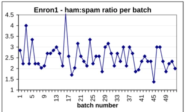
Enron1 - ham:spam ratio per batch

1 1.5 2 2.5 3 3.5 4 4.5 1 5 9 13 17 21 25 29 33 37 41 45 49 batch number

Figure 1: Fluctuation of the ham-spam ratio.

arrive in the order produced by the algorithm above. Fig-ure 1 shows the resulting fluctuation of the ham-spam ratio over batches of 100 adjacent messages each. The first batch contains the “oldest” 100 messages, the second one the 100 messages that “arrived” immediately after those of the first batch, etc. The ham-spam ratio in the entire dataset is 2.45. In each ordered dataset, the incremental retraining and evaluation procedure was implemented as follows:

1. Split the sequence of messages into batches b1, . . . , bl

of k adjacent messages each, preserving the order of arrival. Batchblmay have less thankmessages.

2. Fori= 1 tol−1, train the filter (including attribute selection) on the messages of batches 1, . . . , i, and test it on the messages ofbi+1.

Note that at the end of the evaluation, each message of the dataset (excluding b1) will have been classified exactly once. The number of true positives (TP) is the number of spam messages that have been classified as spam, and sim-ilarly for false positives (FP, ham misclassified as spam), true negatives (TN, correctly classified ham), and false neg-atives (FN, spam misclassified as ham). We set k = 100, which emulates the situation where the filter is retrained every 100 new messages.13 We assume that the user marks as false negatives spam messages that pass the filter, and in-spects periodically for false positives a “spam” folder, where messages identified by the filter as spam end up.

In our evaluation, we used spam recall ( TP

TP+FN) and ham recall ( TN

TN+FP). Spam recall is the proportion of spam mes-sages that the filter managed to identify correctly (how much spam it blocked), whereas ham recall is the proportion of ham messages that passed the filter. Spam recall is the com-plement of spam misclassification rate, and ham recall the complement of ham misclassification rate, the two measures that were used in the _trec 2005 Spam Track. In order to evaluate the differentnbversions across the entire tradeoff between true positives and true negatives, we present the evaluation results by means of _roc curves, plotting sensi-tivity (spam recall) against 1−specificity (the complement of ham recall, or ham misclassification rate). This is the 13

Annb-based filter can easily be retrained on-line, immedi-ately after receiving each new message. We chose k= 100 to make it easier to add in future work additional experi-ments with other learning algorithms, such as_svms, which are computationally more expensive to train.

(6)

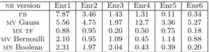
nbversion Enr1 Enr2 Enr3 Enr4 Enr5 Enr6 fb 7.87 3.46 1.43 1.31 0.11 0.34 mvGauss 5.56 4.75 1.97 12.7 3.36 5.27 mn tf 0.88 0.95 0.20 0.50 0.75 0.18 mvBernoulli 2.10 0.95 1.09 0.45 1.14 0.88 mnBoolean 2.31 1.97 2.04 0.43 0.39 0.20

Table 2: Maximum difference (×100) in spam recall across 500, 1000, 3000 attributes forT = 0.5.

nbversion Enr1 Enr2 Enr3 Enr4 Enr5 Enr6

fb 0.61 0.23 1.72 0.54 0.48 0.34

mvGauss 1.17 0.75 5.94 1.77 5.91 4.88

mn tf 2.17 1.38 1.02 0.61 1.70 1.22

mvBernoulli 1.47 0.63 6.37 2.04 2.11 1.22

mnBoolean 0.53 0.68 0.10 0.48 1.36 2.17

Table 3: Maximum difference (×100) in ham recall across 500, 1000, 3000 attributes forT = 0.5.

normal definition of roc analysis, when treating spam as the positive and ham as the negative class.

The _roc curves capture the overall performance of the different nb versions in each dataset, but fail to provide a picture of the progress made by each nb version during the incremental procedure. For this reason, we additionally examine the learning curves of the five methods in terms of the two measures forT = 0.5, i.e., we plot spam and ham recall as the training set increases during the incremental retraining and evaluation procedure.

4. EXPERIMENTAL RESULTS

4.1 Size of attribute set

We first examined the impact of the number of attributes on the effectiveness of the fivenbversions.14 As mentioned above, we experimented with 500, 1000, and 3000 attributes. The full results of these experiments (not reported here) in-dicate that overall the best results are achieved with 3000 attributes, as one might have expected. The differences in effectiveness across different numbers of attributes, however, are rather insignificant. As an example, Tables 2 and 3 show the maximum differences in spam and ham recall, respec-tively, across the three sizes of the attribute set, for each_nb version and dataset, withT = 0.5; note that the differences are in percentage points. The tables show that the differ-ences are very small in all five_nbversions for this threshold value, and we obtained very similar results for all thresholds. Consequently, in operational filters the differences in effec-tiveness may not justify the increased computational cost that larger attribute sets require, even though the increase in computational cost is linear in the number of attributes.

4.2 Comparison of NB versions

Figure 2 shows theroccurves of the five nbversions in each one of the six datasets.15 _{All the curves are for 3000} attributes, and the error bars correspond to 0.95 confidence intervals; we show error bars only at some points to avoid 14

We used a modified version offiltron[18] for our experi-ments, with_weka’s implementations of the five_nbversions;

seehttp://www.cs.waikato.ac.nz/∼ml/weka/.

15_{Please view the figures in color, consulting the on-line} ver-sion of this paper if necessary; seehttp://www.ceas.cc/.

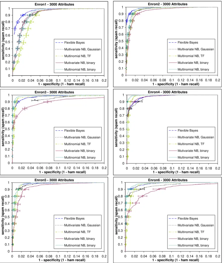
cluttering the diagrams. Since the tolerance of most users on misclassifying ham messages is very limited, we have re-stricted the horizontal axis (1−specificity = 1−ham recall) of all diagrams to [0,0.2], i.e., a maximum of 20% of mis-classified ham, in order to improve the readability of the diagrams. On the vertical axis (sensitivity, spam recall) we show the full range, which allows us to examine what propor-tion of spam messages the five_nbversions manage to block when requesting a very low ham misclassification rate (when 1−specificity approaches 0). The optimal performance point in an_rocdiagram is the top-left corner, while the area un-der each curve (auc) is often seen as a summary of the performance of the corresponding method. We do not, how-ever, believe that standard_aucis a good measure for spam filters, because it is dominated by non-high specificity (ham recall) regions, which are of no interest in practice. Perhaps one should compute the area for 1−specificity ∈ [0,0.2] or [0,0.1]. Even then, however, it is debatable how the area should be computed whenroccurves do not span the entire [0,0.2] or [0,0.1] range of the horizontal axis (see below).

A first conclusion that can be drawn from the results of Figure 2 is that some datasets, such as Enron4, are “easier” than others, such as Enron1. There does not seem to be a clear justification for these differences, in terms of the ham-spam ratio or the ham-spam source used in each dataset.

Despite its theoretical association to term frequencies, in all six datasets the multinomial_nbseems to be doing better when Boolean attributes are used, which agrees with Schnei-der’s observations [25]. The difference, however, is in most cases very small and not always statistically significant; it is clearer in the first dataset and, to a lesser extent, in the last one. Furthermore, the multinomialnbwith Boolean at-tributes seems to be the best performer in 4 out of 6 datasets, although again by a small and not always statistically sig-nificant margin, and it is clearly outperformed only byfbin the other 2 datasets. This is particularly interesting, since many _nb-based spam filters appear to adopt the multino-mialnbwithtfattributes or the multi-variate Bernoullinb (which uses Boolean attributes); the latter seems to be the worst among the_nbversions we evaluated. Among the_nb versions that we tested with normalized tf attributes (fb and the multi-variate Gauss nb), overall fb is clearly the best. However, _fb does not always outperform the other nb version that uses non-Boolean attributes, namely the multinomialnbwithtfattributes.

The_fbclassifier shows signs of impressive superiority in Enron1 and Enron2; and its performance is almost undis-tinguishable from that of the top performers in Enron5 and Enron6. However, it does not perform equally well, com-pared to the top performers, in the other two datasets (En-ron3, Enron4), which strangely include what appears to be the easiest dataset (Enron4). One problem we noticed with fbis that its estimates forp(c|~x) are very close to 0 or 1; hence, varying the threshold T has no effect on the classi-fication of many messages. This did not allow us to obtain higher ham recall (lower 1−specificity) by trading off spam recall (sensitivity) as well as in the othernbversions, which is why thefb roccurves are shorter in some of the diagrams. (The same comment applies to the multi-variate Gauss_nb.) Having said that, we were able to reach a ham recall level of 99.9% or higher withfbin most of the datasets.

Overall, the multinomial_nbwith Boolean attributes and fbobtained the best results in our experiments, but the

(7)

dif-Enron1 - 3000 Attributes 0 0.1 0.2 0.3 0.4 0.5 0.6 0.7 0.8 0.9 1 0 0.02 0.04 0.06 0.08 0.1 0.12 0.14 0.16 0.18 0.2

1 - specificity (1 - ham recall)

s e n s it iv it y ( s p a m r e c a ll ) Flexible Bayes Multivariate NB, Gaussian Multinomial NB, TF Mutivariate NB, binary Multinomial NB, binary Enron2 - 3000 Attributes 0 0.1 0.2 0.3 0.4 0.5 0.6 0.7 0.8 0.9 1 0 0.02 0.04 0.06 0.08 0.1 0.12 0.14 0.16 0.18 0.2

s e n s it iv it y ( s p a m r e c a ll ) Flexible Bayes Multivariate NB, Gaussian Multinomial NB, TF Mutivariate NB, binary Multinomial NB, binary Enron6 - 3000 Attributes 0 0.1 0.2 0.3 0.4 0.5 0.6 0.7 0.8 0.9 1 0 0.02 0.04 0.06 0.08 0.1 0.12 0.14 0.16 0.18 0.2 1 - specificity (1 - ham recall)

s e n s it iv it y ( s p a m r e c a ll ) Flexible Bayes Multivariate NB, Gaussian Multinomial NB, TF Mutivariate NB, binary Multinomial NB, binary

(8)

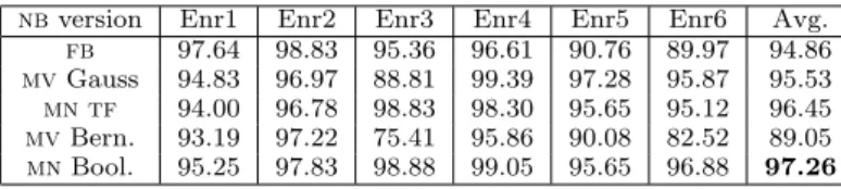
nbversion Enr1 Enr2 Enr3 Enr4 Enr5 Enr6 Avg. fb 90.50 93.63 96.94 95.78 99.56 99.55 95.99 mvGauss 93.08 95.80 97.55 80.14 95.42 91.95 92.32 mn tf 95.66 96.81 95.04 97.79 99.42 98.08 97.13 mvBern. 97.08 91.05 97.42 97.70 97.95 97.92 96.52 mnBool. 96.00 96.68 96.94 97.79 99.69 98.10 97.53

Table 4: Spam recall (%) for 3000 attributes,T = 0.5.

nbversion Enr1 Enr2 Enr3 Enr4 Enr5 Enr6 Avg.

fb 97.64 98.83 95.36 96.61 90.76 89.97 94.86

mvGauss 94.83 96.97 88.81 99.39 97.28 95.87 95.53 mn tf 94.00 96.78 98.83 98.30 95.65 95.12 96.45 mvBern. 93.19 97.22 75.41 95.86 90.08 82.52 89.05 mnBool. 95.25 97.83 98.88 99.05 95.65 96.88 97.26

Table 5: Ham recall (%) for 3000 attributes,T = 0.5.

ferences from the othernb versions were often very small. Taking into account its smoother trade-off between ham and spam recall, and its better computational complexity at run time, we tend to prefer the multinomial nb with Boolean attributes over_fb, but further experiments are necessary to establish its superiority with confidence. For completeness, Tables 4 and 5 list the spam and ham recall, respectively, of the_nbversions on the 6 datasets forT = 0.5, although com-paring at a fixed thresholdT is not particularly informative; for example, two methods may obtain the same results at different thresholds. On average, the multinomial_nbwith Boolean attributes again has the best results, both in spam and ham recall.

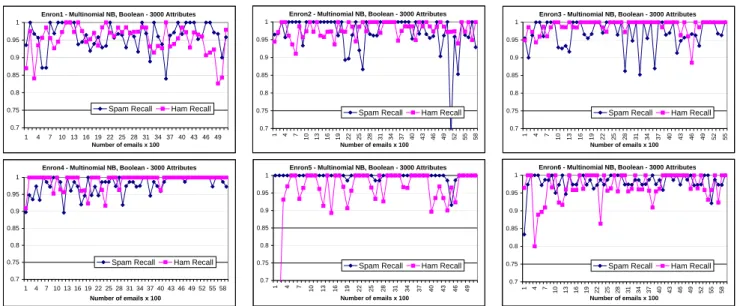
4.3 Learning curves

Figure 3 shows the learning curves (spam and ham recall as more training messages are accumulated over time) of the multinomialnbwith Boolean attributes on the six datasets for T = 0.5. It is interesting to observe that the curves do not increase monotonically, unlike most text classifica-tion experiments, presumably because of the unpredictable fluctuation of the ham-spam ratio, the changing topics of spam, and the adversarial nature of anti-spam filtering. In the “easiest” dataset (Enron4) the classifier reaches almost perfect performance, especially in terms of ham recall, after a few hundreds of messages, and quickly returns to near-perfect performance whenever a deviation occurs. As more training messages are accumulated, the deviations from the perfect performance almost disappear. In contrast, in more difficult datasets (e.g., Enron1) the fluctuation of ham and spam recall is continuous. The classifier seems to adapt quickly to changes, though, avoiding prolonged plateaus of low performance. Spam recall is particularly high and stable in Enron5, but this comes at the expense of frequent large fluctuations of ham recall; hence, the high spam recall may be the effect of a tradeoff between spam and ham recall.

5. CONCLUSIONS AND FURTHER WORK

We discussed and evaluated experimentally in a spam fil-tering context five different versions of the Naive Bayes (_nb) classifier. Our investigation included two versions ofnbthat have not been used widely in the spam filtering literature, namely Flexible Bayes (_fb) and the multinomial _nb with Boolean attributes. We emulated the situation faced by a new user of a personalized learning-based spam filter,

adopt-ing an incremental retrainadopt-ing and evaluation procedure. The six datasets that we used, and which we make publicly avail-able, were created by mixing freely available ham and spam messages in different proportions. The mixing procedure emulates the unpredictable fluctuation over time of the ham-spam ratio in real mailboxes.

Our evaluation included plotting _roc curves, which al-lowed us to compare the different _nb versions across the entire tradeoff between true positives and true negatives. The most interesting result of our evaluation was the very good performance of the two _nb versions that have been used less in spam filtering, i.e., fband the multinomialnb with Boolean attributes; these two versions collectively ob-tained the best results in our experiments. Taking also into account its lower computational complexity at run time and its smoother trade-off between ham and spam recall, we tend to prefer the multinomial_nb with Boolean attributes over fb, but further experiments are needed to be confident. The best results in terms of effectiveness were generally achieved with the largest attribute set (3000 attributes), as one might have expected, but the gain was rather insignificant, com-pared to smaller and computationally cheaper attribute sets. We are currently collecting more data, in a setting that will allow us to evaluate the five_nbversions and other learn-ing algorithms on several real mailboxes with the incremen-tal retraining and evaluation method. The obvious caveat of these additional real-user experiments is that it will not be possible to provide publicly the resulting datasets in a non-encoded form. Therefore, we plan to release them using the encoding scheme of the_pudatasets.

6. REFERENCES

[1] I. Androutsopoulos, J. Koutsias, K. Chandrinos, and C. Spyropoulos. An experimental comparison of Naive Bayesian and keyword-based anti-spam filtering with encrypted personal e-mail messages. In23rd ACM SIGIR Conference, pages 160–167, Athens, Greece, 2000.

[2] I. Androutsopoulos, G. Paliouras, and E. Michelakis. Learning to filter unsolicited commercial e-mail. technical report 2004/2, NCSR “Demokritos”, 2004. [3] R. Beckermann, A. McCallum, and G. Huang.

Automatic categorization of email into folders: benchmark experiments on Enron and SRI corpora. Technical report IR-418, University of Massachusetts Amherst, 2004.

[4] X. Carreras and L. Marquez. Boosting trees for anti-spam email filtering. In4th International Conference on Recent Advances in Natural Language Processing, pages 58–64, Tzigov Chark, Bulgaria, 2001.

[5] P. Domingos and M. Pazzani. On the optimality of the simple Bayesian classifier under zero-one loss.Machine Learning, 29(2–3):103130, 1997.

[6] H. D. Drucker, D. Wu, and V. Vapnik. Support Vector Machines for spam categorization.IEEE Transactions On Neural Networks, 10(5):1048–1054, 1999.

[7] S. Eyheramendy, D. Lewis, and D. Madigan. On the Naive Bayes model for text categorization. In9th International Workshop on Artificial Intelligence and Statistics, pages 332–339, Key West, Florida, 2003. [8] T. Fawcett. In “vivo” spam filtering: a challenge

(9)

Enron1 - Multinomial NB, Boolean - 3000 Attributes 0.7 0.75 0.8 0.85 0.9 0.95 1 1 4 7 10 13 16 19 22 25 28 31 34 37 40 43 46 49 Number of emails x 100

Spam Recall Ham Recall

Enron2 - Multinomial NB, Boolean - 3000 Attributes

0.7 0.75 0.8 0.85 0.9 0.95 1 1 4 7 ₁₀ ₁₃ ₁₆ ₁₉ ₂₂ ₂₅ ₂₈ ₃₁ ₃₄ ₃₇ ₄₀ ₄₃ ₄₆ ₄₉ ₅₂ ₅₅ ₅₈ Number of emails x 100

0.7 0.75 0.8 0.85 0.9 0.95 1 1 4 7 ₁₀ ₁₃ ₁₆ ₁₉ ₂₂ ₂₅ ₂₈ ₃₁ ₃₄ ₃₇ ₄₀ ₄₃ ₄₆ ₄₉ ₅₂ ₅₅ Number of emails x 100

0.7 0.75 0.8 0.85 0.9 0.95 1 1 4 7 10 13 16 19 22 25 28 31 34 37 40 43 46 49 52 55 58 Number of emails x 100

0.7 0.75 0.8 0.85 0.9 0.95 1 1 4 7 ₁₀ ₁₃ ₁₆ ₁₉ ₂₂ ₂₅ ₂₈ ₃₁ ₃₄ ₃₇ ₄₀ ₄₃ ₄₆ ₄₉ Number of emails x 100

0.7 0.75 0.8 0.85 0.9 0.95 1 1 4 7 10 13 16 19 22 25 28 31 34 37 40 43 46 49 52 55 58 Number of emails x 100

Figure 3: Learning curves for the multinomial NB with Boolean attributes andT = 0.5.

problem for KDD.SIGKDD Explorations, 5(2):140–148, 2003.

[9] S. Hershkop and S. Stolfo. Combining email models for false positive reduction. In11th ACM SIGKDD Conference, pages 98–107, Chicago, Illinois, 2005. [10] J. G. Hidalgo. Evaluating cost-sensitive unsolicited

bulk email categorization. In17th ACM Symposium on Applied Computing, pages 615–620, 2002.

[11] J. G. Hidalgo and M. M. Lopez. Combining text and heuristics for cost-sensitive spam filtering. In4th Computational Natural Language Learning Workshop, pages 99–102, Lisbon, Portugal, 2000.

[12] J. Hovold. Naive Bayes spam filtering using

word-position-based attributes. In2nd Conference on Email and Anti-Spam, Stanford, CA, 2005.

[13] J. T. J.D.M. Rennie, L. Shih and D. Karger. Tackling the poor assumptions of Naive Bayes classifiers. In 20th International Conference on Machine Learning, pages 616–623, Washington, DC, 2003.

[14] G. John and P. Langley. Estimating continuous distributions in Bayesian classifiers. In11th

Conference on Uncertainty in Artificial Intelligence, pages 338–345, Montreal, Quebec, 1995.

[15] B. Klimt and Y. Yang. The Enron corpus: a new dataset for email classification research. In15th European Conference on Machine Learning and the 8th European Conference on Principles and Practice of Knowledge Discovery in Databases, pages 217–226, Pisa, Italy, 2004.

[16] A. Kolcz and J. Alspector. SVM-based filtering of e-mail spam with content-specific misclassification costs. InWorkshop on Text Mining, IEEE

International Conference on Data Mining, San Jose, California, 2001.

[17] A. McCallum and K. Nigam. A comparison of event models for naive bayes text classification. InAAAI’98 Workshop on Learning for Text Categorization, pages 41–48, Madison, Wisconsin, 1998.

[18] E. Michelakis, I. Androutsopoulos, G. Paliouras, G. Sakkis, and P. Stamatopoulos. Filtron: a

learning-based anti-spam filter. In1st Conference on Email and Anti-Spam, Mountain View, CA, 2004. [19] P. Pantel and D. Lin. SpamCop: a spam classification

and organization program. InLearning for Text Categorization – Papers from the AAAI Workshop, pages 95–98, Madison, Wisconsin, 1998.

[20] F. Peng, D. Schuurmans, and S. Wang. Augmenting naive bayes classifiers with statistical language models.Information Retrieval, 7:317–345, 2004. [21] M. Sahami, S. Dumais, D. Heckerman, and

E. Horvitz. A Bayesian approach to filtering junk e-mail. InLearning for Text Categorization – Papers from the AAAI Workshop, pages 55–62, Madison, Wisconsin, 1998.

[22] G. Sakkis, I. Androutsopoulos, G. Paliouras,

V. Karkaletsis, C. Spyropoulos, and P. Stamatopoulos. Stacking classifiers for anti-spam filtering of e-mail. In Conference on Empirical Methods in Natural

Language Processing, pages 44–50, Carnegie Mellon University, Pittsburgh, PA, 2001.

[23] G. Sakkis, I. Androutsopoulos, G. Paliouras,

V. Karkaletsis, C. Spyropoulos, and P. Stamatopoulos. A memory-based approach to anti-spam filtering for mailing lists.Information Retrieval, 6(1):49–73, 2003. [24] K.-M. Schneider. A comparison of event models for

Naive Bayes anti-spam e-mail filtering. In10th Conference of the European Chapter of the ACL, pages 307–314, Budapest, Hungary, 2003.

[25] K.-M. Schneider. On word frequency information and negative evidence in Naive Bayes text classification. In 4th International Conference on Advances in Natural Language Processing, pages 474–485, Alicante, Spain, 2004.