EXPLAINING MONDAY RETURNS 1

EXPLAINING MONDAY RETURNS

By

Paul Draper

University of Edinburgh

Krishna Paudyal

University of Durham

Key words

:

JEL classification: G12, G14

1

The authors have benefited from the comments of an anonymous referee, the editor and the seminar participants at the Financial Management Association Conference, Barcelona 1999 and the Multinational Finance Society Conference 1999 Toronto. Please address correspondence to Professor Krishna Paudyal, Department of Economics and Finance, University of Durham, 23-26 Old Elvet, Durham, DH1 3HY, UK. Tel: +44(0)1913747523, Fax: +44(0)1913747289, E-mail. K.N.Paudyal@Durham.ac.uk.

EXPLAINING MONDAY RETURNS

Abstract

The Monday effect is re-examined using two stock indices and a sample of 452 individual stocks that trade on the London Stock Exchange. The results based on conventional test methods reveal a low average return on Monday. Extending the analysis to examine the effects of various possible influences simultaneously, the average Monday return becomes positive and does not differ significantly from the average returns of most other days of the week. Fortnight, ex-dividend day, account period, (bad) news flow, trading activity and bid-ask spread effects are all controlled for. The results broadly support the trading time hypothesis.

EXPLAINING MONDAY RETURNS

1. INTRODUCTION

Day-of-the-week effects in stock returns and particularly, the presence of Monday (or weekend) effects have been reported for many of the worlds' stock markets. Typical studies of the day-of-the-week effect report significant, negative Monday returns and high and positive returns during the middle of the week. Agrawal and Tandon (1994), for example, report evidence of a weekend effect in stock returns in nine countries whilst Dubois and Louvet (1996) suggest that returns are lower at the beginning of the week in a number of stock markets. A variety of hypotheses have been advanced to explain the effect but there has as yet been little agreement as to its cause.

The predominant method used in testing the effect has been to measure Monday returns relative to other days of the week and then to examine and compare the effect within and between samples chosen on the basis of size (small firms), month of the year (January), time of the month (first or second half) or some other criterion. Whilst revealing, such an approach is by its very nature limited in the number of variables that may be considered and prevents consideration of a wide range of effects simultaneously. The method adopted here assumes, following the (sometimes conflicting) research of more than 20 years, that there are a number of variables influencing the Monday return and attempts to explain the effect using not one but several explanatory variables. In the process we are able to support a number of the hypotheses that have been advanced.

Two of the most enduring suggestions for the Monday effect are the calendar time and trading time hypotheses (French 1980). The calendar time hypothesis suggests that the average Monday return should be three times the average returns that occur on other days of the week. In contrast, the trading time hypothesis postulates that the Monday returns should not be significantly different from the returns available on any other day of the week.

The majority of empirical studies have used Friday close to Monday close returns. Such studies are unable to establish whether the negative returns found are due to the absence of trading over the weekend, or to the trading that occurs on Monday. Rogalski (1984) distinguishes between Friday close to Monday open, and Monday

open to Monday close returns. His evidence suggests that the negative returns over the whole Friday to Monday close period occur during the non-trading period from Friday close to Monday open. Other studies, in general, have not confirmed this result. Keim and Stambaugh (1984), for example, provide evidence that returns for one day weekends (Saturday to Monday close) computed from historic NYSE data, are more negative than returns for (the current) two day weekends. Lauterbach and Ungar (1992) reveal that all returns are positive for the Tel Aviv Exchange including Sunday (the market is closed on Friday and Saturday) but note that the Monday return whilst positive is lower than for any other day of the week.

Keim and Stambaugh (1984) for the US and Board and Sutcliffe (1988) for the UK attempt to explain the Monday effect through measurement error (over-estimation of Friday’s closing price and under-estimation of Monday’s closing price). Jaffe and Westerfield (1985) and Board and Sutcliffe (1988) suggest that part of the Monday effect could be explained by the gap between trading and settlement day. Penman (1987) and Damodaran (1989) find evidence to suggest that ‘news’, and in particular bad news released after the closing of the stock market on Friday helps explain the negative Monday returns. Athanassakos and Robinson (1994) examine the impact of clustering of the ex-dividend date on Mondays in Canada but even after correcting for this effect a strong negative Monday effect is observed. They suggest that the day-of-the-week effect is mainly due to news flow, especially of macroeconomic announcements. Abraham and Ikenberry (1994) report evidence that the trading behavior of individual investors appears to be at least one factor contributing to the day-of-the-week effect. Lakonishok and Maberly (1990) note that NYSE trading volume is lower on Mondays than on other days of the week but that individuals tend to trade more. Keim and Stambaugh (1984) suggest that ‘relatively small variations in the bid vs. ask frequency during the week could contribute to day-of-the-week effects in computed returns’ (p.832).

The majority of studies that explore the day-of-the-week effect are based on US experience. This paper explores the day-of-the-week effect for the different UK equity trading system and adjusts returns for a range of inter-related stock market variables including trading activity and bid-ask spread. Inclusion of these variables enables us to clarify the day-of-the-week behavior of the stock market. This study differs from UK studies in a number of respects. We include only data which cover

the market maker system of equity trading on the London Stock Exchange2 (LSE) and examine a number of possible causes of the Monday effect including a variety of market micro-structure explanations arising from trading and settlement procedures, and the impact of ex-dividend days on returns. We analyze not only stock market indices but also the intra-week behavior of a sample of individual stocks that differ considerably in size. We also examine the impact of the time in the month and news variables on the results.

2. SAMPLE AND METHOD

2.1 Data:

Our sample period is taken from the beginning of 19883 until December 1997. Required data are collected from Datastream. Daily closing prices, return indices, bid-price, ask-price, market value, trading volume (number of shares traded) and number of trades are required for all stocks in the sample. Of the constituents (over 800 companies) of the FT-All Share Index the price variables (closing price, return index, bid-price and ask-price) are available for 452 companies and are included in our analysis. For some of these companies data on trading activity (volume of trade, number of trades) are not available for the full sample period and hence are coded as missing observations. Account days and ex-dividend days are collected from a variety of sources including the Stock Exchange Official Yearbook, the Financial Times and Extel. To make this study comparable with previous studies we also include an analysis of two major stock indices notably the FTSE100 index which comprises the 100 largest stocks traded on the London Stock Exchange, and the FT-All Share Index, a broad-based index. Both indices are value weighted.

2

The current system of trading was introduced in October 1986. Studies which pool the pre and post 1986 data suffer from a major structural change in market microstructure. More recently, the introduction of automated trading on the FTSE100 stocks has altered the market structure again.

3

Although the SEAQ market making system was introduced in October 1986 it took some time for experience with the system to become widespread. To avoid possible contamination from such factors the sample is taken from January 1988.

2.2 Theoretical Issues and Development of Model:

A common parametric test of the Monday effect is to estimate the following model

,

)

1

(

å

+

=

D

R

α

α

where Rit is the return of security i in day t; the dummy variables Dj (Tuesday = 1, Wednesday = 2, Thursday = 3, Friday = 4) take the value 1 for the day-of-the-week for which the returns are observed, and zero otherwise, and the error term, ε, is assumed to be normally distributed. The value of α0 in equation (1) represents the Monday average return while the coefficients for the four dummy variables (α1, α2, α3, α4) reflect the average deviations in daily return from the Monday. If there is no day-of-the-week effect in returns the coefficients for the four dummy variables are not significantly different from zero so that the return on day i is not different from the return on Monday. Since the results are likely to be affected by the presence of outliers in the data set we estimate the equation using both OLS and robust regression techniques. The regression approach to testing for seasonality is appealing because of the ease with which additional factors that are thought to affect seasonality can be added to the model. For example, the claim of Wang et. al. (1997) claim that a negative Monday return is more prominent in the second half of the month and is not different from other days’ mean return during the first half of the month, is easily tested by the inclusion of an additional dummy variable (Fortnight) indicating the fortnight of the month. The first 15 calendar days of the month are included in the first fortnight and the remaining days of the month are classified as belonging to the second fortnight.

Until July 1994 the London Stock Exchange operated a system of account periods by dividing the year into a fixed number of periods. Account periods typically began on a Monday and lasted for ten working days to the following Friday. Settlement occurred on the Monday six working days later4. During the account period investors could short

4

A typical account period could be summarised in the following time-line: M1 (start) - - - F1 - - M2 - - - F2 (end) - - M3 - - - F3 - - M4 (settlement)

M1: Monday, start day of a typical account period

F2: Following Friday, last day of a typical account period.

10 working days normally occur between M1 and F2 (inclusive).

sell at no cost whilst transactions at the beginning of the account gave investors an interest free period of three calendar weeks or, on occasions (especially around Christmas and the New Year period), longer. All transactions offered credit for at least six working days but the earlier in the account period the transaction was made the longer the credit period. From July 1994, ten and subsequently in June 1995 five-day rolling settlement periods were adopted. Under the new system every transaction has a fixed credit period of five (previously ten) working days.

Two approaches are adopted to modeling the account period and settlement effects. The first approach distinguishes the beginning of the account from other days and includes a dummy variable (Acc Day) in the regression for the first day of the account. This general approach allows for interest, short selling and other effects on returns. The second approach is more specific and includes an interest variable (Int. Day) in the regression to allow for the number of days of credit available before settlement over the period.

Ex-dividend days in the UK are normally on Mondays. Analysis of ex-dividend days for the sample companies during the sample period suggests that nearly 94 percent of ex-dividend days are Mondays. This alone is sufficient to depress the stock price on Mondays. Comparison of stock returns on ex-dividend Mondays with returns on other Mondays as well a comparison of non ex-dividend Mondays’ returns with the returns on other days of the week should provide greater insight into the day-of-the-week behavior of stock returns. If the ex-dividend effect is responsible for the Monday effect, average returns on non-ex-dividend Mondays should not be different from the average return for other days of the week (trading time hypothesis)5. To examine the effect of the payment of dividends an ex-dividend variable (X-Div Day) is added to the model. This variable takes the value of 1 if the day is an ex-dividend day for the security and 0 otherwise.

(F2). All transactions between M1 and F2 (inclusive) must be settled on M4. This implies that

during a typical Account period investors may not pay for up to 3 weeks. The new Account period started on Monday (M3) and lasted ten days through to the Friday the following week

(F4). Account periods were occasionally longer than ten days when they included a public

holiday.

5

If the calendar time hypothesis is correct then Monday (non-ex-dividend) return will be three times the average return of other days of the week.

Abraham and Ikenberry (1994) test the information processing hypothesis (put forward by Lakonishok and Maberly (1990)) which ‘… suggests that individuals will, in general, be more aggressive sellers of securities early in the trading week, particularly on Mondays following declines in the market the prior Friday.’ (p. 272). Their findings are consistent with this hypothesis and suggest that individuals postpone sell-related investment decisions to the weekend and there is a sell-oriented order flow from individuals early in the trading week. At the same time institutional investors often use Monday mornings to plan strategy so that orders on Monday from institutional investors are reduced. If the information-processing hypothesis is true, Abraham and Ikenberry suggest that a negative relationship should exist between the return on Monday and the degree of individual selling behavior. We might expect the relationship to be more powerful for small companies (where small investors are more significant holders) than for large companies, and, in terms of the hypothesis would expect to see more aggressive selling activity following the receipt of negative information. To examine the information-processing hypothesis we include an additional variable (News) to represent the sign of the return on the prior Friday. For each company this variable takes the value 1 on Monday if the prior Friday return is negative (to represent information revealed in prior trading sessions) and 0 otherwise.

A number of studies have attributed the Monday effect to trading activity. Lakonishok and Maberly (1990) and Abraham and Ikenberry (1994) attribute the negative Monday returns to sell-side pressure from individual investors. Kamara (1995) reports that during a period of increased institutional trading activity (1962-1993) the magnitude of the Monday effect declined significantly while Sias and Starks (1995) indicate that the day-of-the-week effect is more prominent in securities in which institutional investors play a greater role. To examine the day-of-the-week effects resulting from trading activity of stocks traded on the London Stock Exchange two variables, the percentage change in number of trades (Change in NT) and the change in the average size of the order (O/S Change) are included in the regression equation. These two variables taken together provide a measure of liquidity and volume of trading.

Studies of the month-of-the-year effect (Clark et al 1992) have in some cases attributed the high January return to a low bid-ask spread. If the market makers have to increase their quoted spread for some reasons6 they may do so (a) by revising the

6

bid and ask quotes (b) by reducing the bid price or (c) by increasing the ask price. If the revision in bid and ask quote is equal, the quoted price (average of bid and ask) will not be affected. An increase in spread through a reduction in the bid price (keeping the ask price constant) would result in a decline in the quoted price and ultimately reduce the calculated return. Hence the observed intra-week seasonality in stock returns could be due to a change in the quoted spread. In this case we should observe a day-of-the-week effect on spread with a significant increase on Monday. To examine this hypothesis we extend the model to include bid-ask spread.

A number of studies (see Draper and Paudyal (1997)) and the references cited therein) have suggested that on average, January returns are higher than the returns during any other month of the year. To control for the influence of this effect a January dummy (1 if the month is January, 0 otherwise) is added to the model (January).

The integrated model is estimated as

),

2

(

D

X

R

=

β

+

å

β

+

å

β

+

ε

where Ri,t and Dj are defined as in equation (1) and Xj is a vector of additional explanatory variables (outlined above).

The models (various forms of equation-2) are estimated by means of OLS as well as using robust regression procedure. In the robust regression the estimated parameters are free from the effects of extreme outliers and the standard errors are corrected for heteroscedasticity. In general, the results of the two procedures are qualitatively similar7.

the London Stock Exchange.

7

We report results based on the robust regression procedure. If there are significant differences between the estimates from the two methods we report both to show the impact of extreme outliers on the estimates and to compare the results with those reported in earlier studies.

3. THE RESULTS

The literature on the day-of-the-week effect, particularly that based on US experience, provides strong evidence that the average Monday return is negative and the average daily return increases during the second half of the week. In this section we provide evidence from the LSE. We use two measures of return, the total return including dividends and the change in price to test the intra-week pattern of stock market prices. Total return is calculated as the daily change in price plus any dividend due (expressed as a percentage). The change in price (hereafter denoted price change) is the percentage change in price of the security and excludes the dividend. Use of both measures allows us to examine the possible influences of dividends on stock price when the stocks go ex-dividend8. This issue is more thoroughly discussed in section 3.2. Individual companies are analyzed as well as the two stock indices since the use of a return index alone does not allow analysis of the full range of factors that may cause a Monday effect. Our results are categorized into three nested groups. The first set of estimates incorporate the traditional model (equation 1) and seasonality (calendar time) related factors. The second set of estimates contains the variables from the previous set and, in addition, includes the variables representing the institutional factors that may affect daily returns. The final group includes all the variables of the previous models and adds in the variables relating to trading activity and bid-ask spread.

3.1 Monday Return and Seasonal Factors:

Table 1 documents, for compatibility with existing studies, results for the ‘traditional’ model (equation 1). Consistent with the evidence elsewhere in the literature Model 1 indicates that a significant drop in price occurs on Monday and reveals the average price change on Monday to be lower than the average price change on all other days of the week. This result holds both for our sample of stocks and for our indices (FT-All and FTSE 100) and is supported by the results of non-parametric tests (not shown). As in other stock exchanges the Monday effect is present on the LSE. A similar but weaker pattern, though in this case including a positive Monday return, is also observed for total returns (not shown). For both individual companies and index returns the day-of-the-week effect is observed. The average daily returns for each

8

Results for total returns are only reported where they differ qualitatively from those derived from analysis of changes in price.

day-of-the-week are depicted in Figure 1. It shows that on average, based on the individual company sample, Monday price changes are negative and price changes on all other days of the week are significantly higher.

Rogalski (1984) suggested that the negative Monday return occurs during the non-trading period from Friday close to Monday open. However the results from our sample suggest that the bulk (over 94%) of the negative Monday return occur during Monday trading hours. In general, consistent with the typical Monday effect documented in the literature, Monday return is negative only when calculated on a close to close basis. The Friday close to Monday open return (non-trading hours) is negative but is very small relative to the Friday close to Monday close return. Share prices decline during the trading time of each day of the week (open to close) with the largest drop occurring on Monday. Figure 2 illustrates the results and suggests that the Monday effect occur primarily during the trading hours of Monday.

In a recent article Wang et. al. (1997) report that negative Monday returns are more prominent in the second half of the month and that the Monday return is not different from other days’ mean return during the first half of the month9. To examine this proposition and test whether the specific fortnight of the month can explain the observed drop in Monday price, we incorporate our fortnight variable. Consistent with the suggestion of Wang et. al. (1997) the results presented for Model 2 reveal a significant negative effect dependent on the fortnight of the month, and suggest that the average daily price change during the second half of the month is smaller than during the first half of the month. After controlling for the fortnight effect the gap

9

In a preliminary test we split the data into first half of the month and second half of the month samples. The results reveal: (a) the average daily return during the first half of the month is significantly greater than the average return during the second half of the month. (b) The average Monday (total) return during the first half of the month is positive and greater than the return on other days of the week. (c) During the second half of the month the average Monday returns are negative and significantly lower than the average returns on other days of the week. This suggests that the widely documented evidence on the day-of-the-week effect is primarily observed in the second half of the month.

Figure: 2 about here Figure: 1 about here

between the average price change on Monday and other days of the week is reduced substantially10.

Consistent with the results reported elsewhere, the estimates presented for Model 3 reveal that January has a significant positive impact on stock price changes. However, even after controlling for the January effect we still observe a significant drop in stock prices on Monday and average price changes on other days of the week are significantly higher than for Monday.

To examine the robustness of the observed results we re-estimated all the models using total returns as the dependent variable. The estimates reveal that the average Monday total return is significantly greater than zero. However, under all three models the average Monday total return remains lower than for any other day of the week. Further, consistent with the results reported above and the findings of Wang et al (1997), the Monday effect is more prominent in the second half of the month and once this is adjusted for the difference between the average Monday total return and the return on other days reduces substantially. The significantly lower average Monday return (whether measured by the change in price or total return) is not consistent with the competing trading time or calendar time hypotheses.

3.2 Monday Return and Institutional Factors:

A number of prior studies (Jaffe and Westerfield (1985) and Board and Sutcliffe (1988)) attribute negative Monday returns to the account period (i.e. interest free period) that was a feature of the London Stock Exchange until 1994. We find in Model 4 that the beginning of the account has a significant positive impact on stock returns. However, even after controlling for an account effect the average Monday price change remains significantly lower than zero whilst the average price change for any other day of the week is positive and greater than zero.

10

The low adjusted R-square reported in the table is common in models which use dummy variables alone as explanatory variables. In effect, dummies simply capture the step changes in mean of the dependent variable and do not capture the variation of daily returns. Therefore, a low adjusted R-square is not unexpected.

The Monday effect is more prominent for returns calculated as price changes than returns calculated including dividends. This suggests that the payment of dividends may be a factor in the Monday effect. In normal circumstances the fall in the share price on the ex-dividend day should be close to the size of the dividend payment11. Analysis of ex-dividend days of the sample companies during the sample period suggests that nearly 94 percent of ex-dividend days are Mondays. This alone is sufficient to depress the stock price on Mondays. To control for the effect of dividend payment on stock returns we introduce an additional explanatory variable in the model to represent the ex-dividend day. As anticipated, the results for Model 5 reveal that the ex-dividend day dummy has a significant negative impact on the daily stock price change. After controlling for the ex-dividend day effect the size of negative Monday return is reduced to less than half of its original estimate. A large part of the observed Monday effect is explained by the ex-dividend day12 and it is apparent that the payment of dividend is a major factor in reducing the average Monday return. Estimates for Model 7 (last columnn) derived for total returns confirm the importance of the ex-dividend day effect but the coefficient is approximately half the size and positive.

An alternative explanation of the Monday effect is provided by the information-processing hypothesis. Consistent with its proposition Abraham and Ikenberry (1994) report that ‘overall Monday return is (and continues to be) negative, it is substantially the consequence of information revealed in prior trading sessions, particularly on Fridays.’ (pp. 275-276). Similarly, Bessembinder and Hertzel (1993) note that the autocorrelation between Monday’s return with the prior Friday’s return has been unusually high for at least 100 years. This suggests that stocks with a

11

A one-to-one relationship between the dividend and price change is unlikely to occur since even when a stock goes ex dividend, the dividend payment is not received by shareholders until a number of weeks later.

12

A comparison of average Monday price changes between ex-dividend Mondays and other Mondays revealed various features. (a) There is a significant difference in the average change in price of stocks on ex-dividend Mondays and other Mondays. (b) The average change in price on non-ex-dividend Mondays during the first half of the month is positive while it is negative during the second half of the month. These results indicate that the Monday effect (especially during the first half of the month) is primarily due to the ex-dividend days. Once again, these results suggest that the ex-dividend day contributes significantly to the observed Monday effect. However, it does not explain all of it.

negative Friday return should have a lower Monday return. Our estimates of Model 6 indicate that this News variable exerts a significant negative impact on daily returns. This finding is consistent with the prediction of the information-processing hypothesis. More interestingly, once the effect of this factor is taken into account the average Monday return (both total return and price change) becomes significantly greater than zero. Moreover, the average returns on Tuesday and Wednesday are not significantly different from the return on Mondays, while the average return on Thursdays and Fridays are significantly lower than the estimate for Monday. Thus, once allowance is made for the fortnight, ex-dividend day and news effects the average Monday return (however measured) is not materially different from the average returns on others days of the week. This evidence provides support for the trading time hypothesis where average returns on all trading days of the week are expected to be equal.

The effect of firm size on stock returns is well documented in the finance literature and Draper and Paudyal (1997) report that stock return seasonality is related to firm size. Motivated by this relationship we extend our equation (2) to incorporate a market capitalization variable. The results from Model 7 (price change), reveal that firm size has a significant positive impact on price changes However, although, the firm size variable has a significant positive impact on daily returns, its influence on the day-of-the-week effect remains negligible13.

3.3 Monday Return and Trading Activity:

An initial examination of trading activity reveals a substantial difference in the rate of change of the volume of trade over the days of the week and hence supports the possibility of a day-of-the-week effect in trading volume. Preliminary estimates (not reported) reveal that the average trading volume declines sharply on Monday and increases on Tuesday. A similar pattern is observed in the average size of the order and number of trades. However, the Monday drop in number of trades in relatively

13

With a view to exploring further the possibility of a size effect on Monday returns we construct 4 equally weighted portfolios on the basis of the market capitalisation of the sample stocks. The results reveal that the Monday effect is more prominent in larger firms than in smaller firms. Of 452 sample companies 369 firms have negative Monday returns while 83 firms have positive returns on Mondays. The positive Monday return occurs more frequently for smaller firms than for larger firms. On average, the negative Monday return is much bigger for larger firms and the positive return is relatively smaller.

small and hence the effect on volume comes mainly through the average size of the order. For liquidity and information flow reasons these variables are likely to impact daily returns.

An increase in the number of trades implies many active participants and therefore less information asymmetry. As a result the liquidity level of the stock is enhanced and,

ceteris paribus, the return may be expected to increase. On the other hand, increased size of order from a limited number of market participants implies that those traders possess additional information not available to the market in general. Consequently, the market makers may widen their spread resulting possibly in reduced returns14. Hence, a negative relationship between the observed return and changes in average size of the order flow may be expected. Thus to examine the day-of-the-week effect on returns we extend our model to include changes in the number of trades and average size of order.

A preliminary analysis reveals that the relative bid-ask spread changes significantly over the days of the week. Estimates indicate that the average relative spread on Monday is 2.237 percent of share price. This is significantly larger than the relative spreads on all other days of the week. During the week the spread declines gradually and reaches its lowest level on Friday (2.210 percent)15. Motivated by the observed day-of-the-week pattern on spread we extend our regression equation to include the spread variable, measured by ‘spread as percentage of price’. A negative relationship between return and bid-ask spread is expected16.

14

Normally, these conditions affect the adverse selection cost component of the quoted bid-ask spread. If demand is from sell side investors the price will be revised downward while it would be revised upwards if the demand is from buy side investors. Depending upon the nature of demand, the market makers are likely to widen their spread by adjusting one side of the price (bid or ask). This causes a change in the quoted price of the stock.

15

Variation in relative spread could result from a constant spread in pence but changes in stock price. Thus the largest proportional spread on Monday could be due to the decrease in price. To examine this we analysed the absolute spread and found that the quoted spread is highest on Monday, declines gradually during the week and reaches its lowest level on Friday. This is consistent with the pattern of proportional spread.

16

Multicollinearity could be a problem here as the trading activity and spreads may have some relationship. However, the estimation did not reveal any symptom of multicollinearity

As anticipated, the results indicate that the number of trades has a significant positive impact on daily returns. An inverse relationship is revealed between daily returns and the change in order-size and proportional spread. After controlling for the additional effect of trading activity variables the size of the average Monday return increases substantially17 as revealed by Models 8 and 10. These results are consistent with our expectations and suggest that an increased order size is treated as an information based trade with market makers increasing the adverse selection cost component of spread. Similarly, the inverse relationship between spread and returns implies that the decreased Monday return can, in part, be explained by the increased spread. After adjusting for the effects of trading variables the average Monday return is significantly greater than zero and not significantly different from the average return on Tuesday18. The average returns for other days of the week are statistically significantly different from the average Monday return but the difference is very small compared to the difference suggested by the results for the standard dummy regression model given by Model 1. Firm size displays a significant positive impact on daily returns but has as Models 7 and 10 reveal only a marginal role to play in explaining the day-of-the-week effect.

In summary, the results based on traditional test methods suggest that the average Monday return is much lower (negative if the change in price alone is considered)

(see Greene 1997).

17

An alternative variable to the Account Day dummy is the number of interest free days from purchasing a security until settlement. Although it has a significant positive impact on daily returns it does not capture the Monday effect as well as the dummy variable for the beginning of the account day (see Model 9).

18

Further analysis reveals that the negative Monday return is coincidental with a decline in trading activity. The Monday effect is also more prominent during week 4 of the month. Trading activity in the final week of December (from 22nd onwards) is thin. Evidence confirms that the largest drop in trading activity (measured on average per trading day basis) occurs during the fourth week of December. To examine whether the Monday effect in week 4 is primarily due to the reduced trading in the fourth week of December, we compare the mean return for the period December 23-31 with the mean return for other days of the month. Although the mean Monday return during this festive season is smaller, it is not negative. The evidence of positive returns in December is consistent with the findings of Draper and Paudyal (1997).

than the average return for other days of the week. However, when allowance is made for the various factors that have been suggested as affecting returns the average Monday return becomes very close to the average returns of other days of the week, supporting the trading time hypothesis.

3.4 Annual variation in the Monday effect:

To examine the stability of the pattern of returns Model 7 was re-estimated for each year in the sample (1988 to 1997).

Figure 3 depicts estimates for Model 7. For the years between 1988 and 1993 the average (adjusted) Monday returns (change in price as well as total returns) are either negative or statistically insignificant. Since 1994 the average (adjusted) Monday return is significantly greater than zero and larger than average return for any other day of the week. This suggests that the Monday returns can be explained with the help of institutional factors the pattern of which has changed in recent years. ‘News’ and ‘ex-dividend date’ variables have inverse (significant) impact on returns in the sample years. The finding of Wang et. al. (1997) indicating Monday return to be more prominent in the second half of the month, is here seen to be year specific. In summary, the Monday effect is not stable over the years.

4. CONCLUSIONS:

The day-of-the-week effect in stock returns is examined on two value weighted stock price (return) indices and on a sample of 452 stocks traded on the LSE. Consistent with the evidence documented in the literature the results reveal a significant day-of-the-week effect in stock returns with a negative average Monday return. The observed Monday effect is more prominent during the second half of the month, week 4 having a dominant role. Analysis of trading activity reveals that on Monday all three measures of trading activity (Volume of trade, Number of trades and Average size of order flow) decline significantly. The relative bid-ask spread also reveals a day-of-the-week pattern and tends to decline gradually from Monday to Friday.

A number of alternative hypotheses attempting to explain the Monday effect are tested using a series of nested regression models. The models are estimated using robust regression procedure to minimize the impact of outliers in the data. Estimates

of the effect of calendar seasonality related variables (day-of-the-week, fortnight of the month and January effect) reveal that the daily return is significantly inversely related to the fortnight of the month. After controlling for the fortnight effect the difference between average Monday return and returns on other days of the week narrows substantially.

The effects of account period, ex-dividend day and a news (bad) factor are also important. The estimates reveal that the account day has a significant positive impact on stock return while the ex-dividend day and news factors have an inverse impact. The ex-dividend day and news (bad) effects alter the sign of the average Monday return, which switches from negative to positive. The average Monday return is found to not differ significantly from the average return on Tuesday, Wednesday and Thursday. The average Friday return remains marginally (though significantly) lower than Monday return.

The model is further extended to incorporate the trading activity variables (Number of trades and Average size of order flow) and proportional spread in the equation. As anticipated we find a positive relationship between the number of trades and stock returns. Similarly, significant negative effects of order size and spread are observed. Once again when the effects of these variables on stock returns are allowed for (in addition to the variables described above) the average Monday return increases further and becomes closer to the average return of most other days of the week. Any remaining difference is negligible.

Our findings suggest that the well documented Monday effect in the UK is caused by a combination of various factors, especially the fortnight of the month, account settlement day, ex-dividend day, arrival of (bad) news on Fridays, trading activity and bid-ask spread. Once we control for the possible effects of these factors the average Monday return becomes insignificantly different from the average return of other days of the week. This evidence provides support for the trading time hypothesis

REFERENCES

Abraham, A. and D. Ikenberry (1994), The individual investor and the weekend effect, Journal of Financial and Quantitative Analysis 29, 263-277.

Agrawal, A. and K. Tandon (1994), Anomalies or illusions? Evidence from stock markets in eighteen countries, Journal of International Money and Finance

13, 83-106.

Athanassakos, G. and M. J. Robinson (1994), The Day-of-the-week anomaly: The Toronto Stock Exchange experience, Journal of Business Finance & Accounting 21, 833-856.

Bessembinder, H. and M. Hertzel (1993), Return autocorrelations around nontrading days, Review of Financial Studies 6, 155-189.

Board, J. L. and C. M. Sutcliffe (1988), The weekend effect in the UK stock market returns, Journal of Business Finance and Accounting 15, 199-213.

Clark, R. A., J.J. McConnell, and M. Singh (1992), Seasonalities in NYSE bid-ask spreads and stock returns in January, Journal of Finance 47, 1999-2013.

Damodaran, A. (1989), The weekend effect in information releases: A study of earnings and dividend announcements, Review of Financial Studies 2, 607-623.

Draper, P. and K. Paudyal (1997), Microstructure and seasonality in the UK equity market, Journal of Business Finance and Accounting 24, 1177-1204.

Dubois, M. and P. Louvet (1996), The day-of-the-week effect: The international evidence, Journal of Banking and Finance 20, 1463-1484.

French, K. (1980), Stock returns and the weekend effect, Journal of Financial Economics 8, 55-70.

Jaffe, J. and R. Westerfield (1985), Patterns in Japanese common stock returns: Day-of-the-week and turn-of-the-year effects, Journal of Financial and Quantitative Analysis 20, 261-272.

Kamara, A. (1995), New evidence on the Monday seasonal in stock returns, Working Paper, University of Washington.

Keim, D. and R. Stambaugh (1984), A further investigation of week-end effect in stock returns, Journal of Finance 39, 819-840.

Lakonishok, J. and E. Maberly (1990), The week-end effect trading patterns of individual and institutional investors, Journal of Finance 45, 231-243.

Lauterbach, B and M Ungar (1992), Calendar anomalies: some perspectives from the behavior of the Israeli stock market, Applied Financial Economics 2, 57-60.

Menyah, K. and K. Paudyal (1996), The determinants and dynamics of bid-ask spreads on the London Stock Exchange, Journal of Financial Research 19, 377-394.

Penman, S. (1987), The distribution of earnings news over time and seasonalities in aggregate stock returns, Journal of Financial Economics 18, 199-228.

Rogalski, R. (1984), New findings regarding day-of-the-week returns over trading and non-trading periods, Journal of Finance 39, 1603-1614.

Sias, R. W. and L. Starks (1995), The day-of-the-week anomaly: The role of institutional investors, Financial Analysts Journal 51, 58-67.

Wang, K., Y. Li, and J. Erickson (1997), A new look at the Monday effect, Journal of Finance 52, 2171-2186.

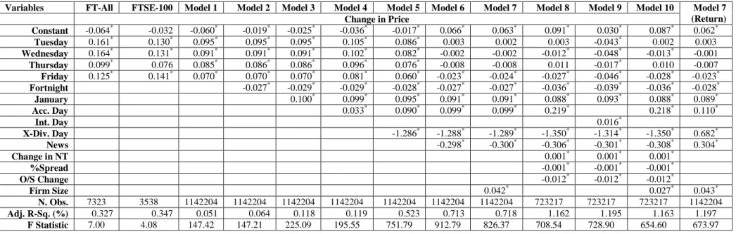
Table 1 Daily Returns, Calendar Time, Institutional Factors and Trading Activity (Robust Regression)

Variables FT-All FTSE-100 Model 1 Model 2 Model 3 Model 4 Model 5 Model 6 Model 7 Model 8 Model 9 Model 10

Change in Price Model 7 (Return) Constant -0.064* -0.032 -0.060* -0.019* -0.025* -0.036* -0.017* 0.066* 0.063* 0.091* 0.030* 0.087* 0.062* Tuesday 0.161* 0.130* 0.095* 0.095* 0.095* 0.105* 0.086* 0.003 0.002 0.003 -0.043* 0.002 0.003 Wednesday 0.164* _0.131* _0.091* _0.091* _0.091* _0.102* _0.082* _{-0.002 -0.002 -0.012}* _-0.048* _-0.013* _-0.001 Thursday 0.099* 0.076 0.085* 0.086* 0.086* 0.096* 0.076* -0.008 -0.008 0.011 -0.017* 0.010 -0.007 Friday 0.125* 0.141* 0.070* 0.070* 0.070* 0.081* 0.060* -0.023* -0.024* -0.027* -0.046* -0.028* -0.023* Fortnight -0.027* -0.029* -0.029* -0.028* -0.027* -0.027* -0.036* -0.039* -0.036* -0.028* January 0.100* 0.099* 0.095* 0.091* 0.091* 0.088* 0.093* 0.088* 0.089* Acc. Day 0.033* 0.090* 0.099* 0.099* 0.219* 0.218* 0.110* Int. Day 0.016* X-Div. Day -1.286* _-1.288* _-1.289* _-1.350* _-1.314* _-1.350* _0.682* News -0.298* -0.300* -0.306* -0.301* -0.308* 0.304* Change in NT 0.001* 0.001* 0.001* %Spread -0.001* -0.001* -0.001* O/S Change -0.012* -0.012* -0.012* Firm Size 0.042* 0.027* 0.043* N. Obs. 7323 3538 1142204 1142204 1142204 1142204 1142204 1142204 1142204 723217 723217 723217 1142204 Adj. R-Sq. (%) 0.327 0.347 0.051 0.064 0.118 0.119 0.523 0.713 0.718 1.162 1.195 1.163 1.197 F Statistic 7.00 4.08 147.42 147.21 225.09 195.55 751.79 912.79 826.37 708.54 728.90 654.60 673.97

Notes: Daily stock returns (changes in price only and total return) are regressed against a set of selected explanatory variables (equation 2) using a robust

regression procedure. With the exception of Model 7 the results for price changes only are reported. Estimates for two indices, the FT-All and FTSE-100 provide comparison with the results reported in the literature. Models 1, 2 and 3 incorporate only the calendar time variables. Models 4 to 7 include calendar time variables as well as institutional factors that are likely to influence the Monday returns. The final set of models (8, 9, and 10) includes trading activity variables and bid-ask spread in addition to the variables incorporated in previous set of models. In the interest of space T-statistics are not included in the table. * Indicates statistically significant at 5 percent or better. The F-Statistics are statistically significant in all models indicating their overall significance. The low adjusted r squared statistics are a reflection of the dummy variable methodology which captures the change in the mean of the dependent variable.

-0.08 -0.06 -0.04 -0.02 0.00 0.02 0.04 0.06 Re tu rn in %

Mon Tue W ed Thu Fri

D ay of the Week

Figure: 1 Average Daily Returns

(without controlling for the effeects of other variables)

Price Change Total Return ` -0.08 -0.06 -0.04 -0.02 0.00 0.02 0.04 0.06 0.08 0.10 R e tu rn in %

Mon Tue Wed Thu Fri Day of the Week

Figure: 2

Average Daily Returns During Trading and Nontrading Hours (without controlling for the effects of other variables)

Non-Trading Hours Trading Hours Close to Close

-0.10 -0.05 0.00 0.05 0.10 0.15 0.20 0.25 Re tu rn in % 1988 1989 1990 1991 1992 1993 1994 1995 1996 1997 Sample Year Figure: 3 Average Monday return

(After controlling for the effects of other variables (Model: 7))