Renewable Electricity
Futures Study
End-use Electricity Demand
Volume 3 of 4 Volume 2 PDF Volume 3 PDF Volume 1 PDF Volume 4 PDFRenewable Electricity Futures Study
Edited By
Hand, M.M.
National Renewable Energy LaboratoryBaldwin, S.
U.S. Department of EnergyDeMeo, E.
Renewable Energy Consulting Services, Inc.Reilly, J.
Massachusetts Institute of TechnologyMai, T.
National Renewable Energy LaboratoryArent, D.
Joint Institute for Strategic Energy Analysis
Porro, G.
National Renewable Energy LaboratoryMeshek, M.
National Renewable Energy LaboratorySandor, D.
National Renewable Energy LaboratorySuggested Citations
Renewable Electricity Futures Study (Entire Report)
National Renewable Energy Laboratory. (2012). Renewable Electricity Futures Study. Hand, M.M.; Baldwin, S.; DeMeo, E.; Reilly, J.; Arent, D.; Porro, G.; Mai, T.; Meshek, M.; Sandor, D. eds. 4 vols. NREL/TP-6A20-52409. Golden, CO: National Renewable Energy Laboratory.
http://www.nrel.gov/analysis/re_futures/. Volume 3: End-Use Electricity Demand
Hostick, D.; Belzer, D.B.; Hadley, S.W.; Markel, T.; Marnay, C.; Kintner-Meyer, M. (2012). End-Use Electricity Demand. Vol. 3 of Renewable Electricity Futures Study. NREL/TP-6A20-52409-3. Golden, CO: National Renewable Energy Laboratory.
Renewable Electricity
Futures Study
Volume 3: End-Use
Electricity Demand
Donna Hostick,
1David B. Belzer,
1Stanton W. Hadley,
2Tony Markel,
3Chris Marnay,
4and
Michael Kintner-Meyer
11
Pacific Northwest National Laboratory
2Oak Ridge National Laboratory
3
National Renewable Energy Laboratory
4Lawrence Berkeley National Laboratory
NOTICE
This report was prepared as an account of work sponsored by an agency of the United States government. Neither the United States government nor any agency thereof, nor any of their employees, makes any warranty, express or implied, or assumes any legal liability or responsibility for the accuracy, completeness, or usefulness of any information, apparatus, product, or process disclosed, or represents that its use would not infringe privately owned rights. Reference herein to any specific commercial product, process, or service by trade name, trademark, manufacturer, or otherwise does not necessarily constitute or imply its endorsement, recommendation, or favoring by the United States government or any agency thereof. The views and opinions of authors expressed herein do not necessarily state or reflect those of the United States government or any agency thereof.
Available electronically at http://www.osti.gov/bridge
Available for a processing fee to U.S. Department of Energy and its contractors, in paper, from:
U.S. Department of Energy
Office of Scientific and Technical Information P.O. Box 62
Oak Ridge, TN 37831-0062 phone: 865.576.8401 fax: 865.576.5728
email: mailto:[email protected]
Available for sale to the public, in paper, from: U.S. Department of Commerce
National Technical Information Service 5285 Port Royal Road
Springfield, VA 22161 phone: 800.553.6847 fax: 703.605.6900
email: [email protected]
online ordering: http://www.ntis.gov/help/ordermethods.aspx
Perspective
The Renewable Electricity Futures Study (RE Futures) provides an analysis of the grid integration opportunities, challenges, and implications of high levels of renewable electricity generation for the U.S. electric system. The study is not a market or policy assessment. Rather, RE Futures examines renewable energy resources and many technical issues related to the operability of the U.S. electricity grid, and provides initial answers to important questions about the integration of high penetrations of renewable electricity technologies from a national
perspective. RE Futures results indicate that a future U.S. electricity system that is largely powered by renewable sources is possible and that further work is warranted to investigate this clean generation pathway. The central conclusion of the analysis is that renewable electricity generation from technologies that are commercially available today, in combination with a more flexible electric system, is more than adequate to supply 80% of total U.S. electricity generation in 2050 while meeting electricity demand on an hourly basis in every region of the United States. The renewable technologies explored in this study are components of a diverse set of clean energy solutions that also includes nuclear, efficient natural gas, clean coal, and energy
efficiency. Understanding all of these technology pathways and their potential contributions to the future U.S. electric power system can inform the development of integrated portfolio scenarios. RE Futures focuses on the extent to which U.S. electricity needs can be supplied by renewable energy sources, including biomass, geothermal, hydropower, solar, and wind.
The study explores grid integration issues using models with unprecedented geographic and time resolution for the contiguous United States. The analysis (1) assesses a variety of scenarios with prescribed levels of renewable electricity generation in 2050, from 30% to 90%, with a focus on 80% (with nearly 50% from variable wind and solar photovoltaic generation); (2) identifies the characteristics of a U.S. electricity system that would be needed to accommodate such levels; and (3) describes some of the associated challenges and implications of realizing such a future. In addition to the central conclusion noted above, RE Futures finds that increased electric system flexibility, needed to enable electricity supply-demand balance with high levels of renewable generation, can come from a portfolio of supply- and demand-side options, including flexible conventional generation, grid storage, new transmission, more responsive loads, and changes in power system operations. The analysis also finds that the abundance and diversity of U.S. renewable energy resources can support multiple combinations of renewable technologies that result in deep reductions in electric sector greenhouse gas emissions and water use. The study finds that the incremental cost associated with high renewable generation is comparable to published cost estimates of other clean energy scenarios. Of the sensitivities examined,
improvement in the cost and performance of renewable technologies is the most impactful lever for reducing this incremental cost. Assumptions reflecting the extent of this improvement are based on incremental or evolutionary improvements to currently commercial technologies and do not reflect U.S. Department of Energy activities to further lower renewable technology costs so that they achieve parity with conventional technologies.
RE Futures is an initial analysis of scenarios for high levels of renewable electricity in the United States; additional research is needed to comprehensively investigate other facets of high
renewable or other clean energy futures in the U.S. power system. First, this study focuses on renewable-specific technology pathways and does not explore the full portfolio of clean technologies that could contribute to future electricity supply. Second, the analysis does not attempt a full reliability analysis of the power system that includes addressing sub-hourly, transient, and distribution system requirements. Third, although RE Futures describes the system characteristics needed to accommodate high levels of renewable generation, it does not address the institutional, market, and regulatory changes that may be needed to facilitate such a
transformation. Fourth, a full cost-benefit analysis was not conducted to comprehensively evaluate the relative impacts of renewable and non-renewable electricity generation options. Lastly, as a long-term analysis, uncertainties associated with assumptions and data, along with limitations of the modeling capabilities, contribute to significant uncertainty in the implications reported. Most of the scenario assessment was conducted in 2010 with assumptions concerning technology cost and performance and fossil energy prices generally based on data available in 2009 and early 2010. Significant changes in electricity and related markets have already occurred since the analysis was conducted, and the implications of these changes may not have been fully reflected in the study assumptions and results. For example, both the rapid development of domestic unconventional natural gas resources that has contributed to historically low natural gas prices, and the significant price declines for some renewable technologies (e.g., photovoltaics) since 2010, were not reflected in the study assumptions.
Nonetheless, as the most comprehensive analysis of U.S. high-penetration renewable electricity conducted to date, this study can inform broader discussion of the evolution of the electric system and electricity markets toward clean systems.
The RE Futures team was made up of experts in the fields of renewable technologies, grid integration, and end-use demand. The team included leadership from a core team with members from the National Renewable Energy Laboratory (NREL) and the Massachusetts Institute of Technology (MIT), and subject matter experts from U.S. Department of Energy (DOE) national laboratories, including NREL, Idaho National Laboratory (INL), Lawrence Berkeley National Laboratory (LBNL), Oak Ridge National Laboratory (ORNL), Pacific Northwest National Laboratory (PNNL), and Sandia National Laboratories (SNL), as well as Black & Veatch and other utility, industry, university, public sector, and non-profit participants. Over the course of the project, an executive steering committee provided input from multiple perspectives to support study balance and objectivity.
RE Futures is documented in four volumes of a single report: Volume 1 describes the analysis approach and models, along with the key results and insights; Volume 2 describes the renewable generation and storage technologies included in the study; This volume—Volume 3—presents end-use demand and energy efficiency assumptions; and Volume 4 discusses operational and institutional challenges of integrating high levels of renewable energy into the electric grid.
List of Acronyms and Abbreviations
°C degrees Celsius
AEO Annual Energy Outlook
BA balancing area
BAU business-as-usual Btu British thermal unit
CO2 carbon dioxide
DOE U.S. Department of Energy
EERE U.S. DOE Office of Energy Efficiency and Renewable Energy EIA Energy Information Administration
EPA U.S. Environmental Protection Agency EPRI Electric Power Research Institute FERC Federal Energy Regulatory Commission FHA Federal Highway Administration
ft2 square foot/feet
GW gigawatt(s)
HVAC heating, ventilation, and air conditioning IEA International Energy Agency
kW kilowatt(s) kWh kilowatt-hour(s) LDC load duration curve
MW megawatt(s)
NAS National Academy of Sciences NEMS National Energy Modeling System
NERC North American Electric Reliability Corporation PEV plug-in electric vehicle
PHEV plug-in hybrid electric vehicle
ReEDS Regional Energy Deployment System RE Futures Renewable Electricity Futures Study TES thermal energy storage
TWh terawatt-hour(s) W/ft2
Watts per square foot
Table of Contents
Perspective ... iii List of Acronyms and Abbreviations ... v Introduction ... xi Chapter 13. General Assumptions ... 13-1 Chapter 14. Potential Impact of Carbon Mitigation Measures and Climate Change on Electricity
Demand ... 14-1 Chapter 15. Resulting Scenarios ... 15-1 Chapter 16. Building Sector Electricity Demand ... 16-1 16.1 Low-Demand Baseline... 16-1 16.2 High-Demand Baseline ... 16-3 16.3 Comparison of Projected Energy Intensities ... 16-3 Chapter 17. Industrial Demands and Energy Efficiency ... 17-1 17.1 Low-Demand Baseline... 17-1 17.2 High-Demand Baseline ... 17-2 17.3 Comparison of Projected Energy Intensities ... 17-3 17.4 Combined Cooling, Heating, and Power within the Industrial Sector ... 17-4 Chapter 18. Transportation Demands ... 18-1 18.1 Low-Demand Baseline... 18-1 18.2 High-Demand Baseline ... 18-3 18.3 Comparison to Other Studies ... 18-3 Chapter 19. Hourly Electricity Demand for 2050 ... 19-1 Chapter 20. Supply Curves for Thermal Storage ... 20-1 Chapter 21. Demand Response Capability ... 21-1 Conclusion ... Conclusion-1 Appendices ... Appendices-1 Appendix G. Comparisons to Other Studies ... G-1 Appendix H. Development of Building Load Curves and Hourly Schedules ... H-1 Appendix I. Development of Industrial Load Curves and Hourly Schedules ... I-1 Appendix J. Combined Cooling, Heating, and Power within the Industrial Sector ... J-1 Appendix K. Transportation Electrification Load Development ... K-1 Appendix L. Cost Functions for Thermal Energy Storage in Commercial Buildings ... L-1 Appendix M. Development of Demand Response Amounts ... M-1 Appendix N. Hourly Load Shapes ... N-1 References for Volume 3 ... References-1
List of Figures
Figure 15-1. Total electricity demand, 2010–2050 ... 15-2 Figure 15-2. Total electricity demand, 2010–2050: High Demand (high) and Low Demand
(low) by sector ... 15-3 Figure 15-3. Historical and projected electricity demand assumptions in low-demand and
high-demand scenarios ... 15-3 Figure 16-1. Residential electricity intensities from six studies, including RE Futures ... 16-4 Figure 16-2. Commercial electricity intensities from six studies, including RE Futures .... 16-4 Figure 17-1. Industrial electricity purchases under the High-Demand Baseline and
Low-Demand Baseline ... 17-2 Figure 17-2. Industrial electricity intensities from five studies, including RE Futures ... 17-4 Figure 18-1. Technology market penetration scenarios ... 18-3 Figure 19-1. High-demand hourly load profile, 2050 ... 19-1 Figure 19-2. Low-demand hourly load profile, 2050 ... 19-3 Figure G-1. Comparison of residential electricity intensities from various studies ... G-8 Figure G-2. Comparison of commercial electricity intensities from various studies ... G-9 Figure G-3. Comparison of industrial electricity intensities from various studies ... G-10 Figure H-1. Electricity intensities for residential building segments in the Low-Demand
Baseline ... H-7 Figure H-2. Electricity intensities for residential buildings: High-Demand Baseline vs.
Low-Demand Baseline ... H-7 Figure H-3. Electricity intensities for commercial building segments in the Low-Demand
Baseline ... H-8 Figure H-4. Electricity intensities for commercial sector: High-Demand Baseline vs.
Low-Demand Baseline ... H-8 Figure H-5. Aggregate residential sector electricity projections: High-Demand Baseline vs.
Low-Demand Baseline... H-10 Figure H-6. Aggregate commercial sector electricity projections: High-Demand Baseline vs.
Low-Demand Baseline... H-10 Figure H-7. Electricity market module regions from the National Energy Modeling System,
also used by the Regional Energy Deployment System ... H-23 Figure I-1. Industrial electricity purchases by sector in the High-Demand Baseline ... I-2 Figure I-2. Industrial electricity purchases by sector in the Low-Demand Baseline ... I-2 Figure I-3. Sectors’ electricity purchased per dollar output from the High-Demand Baseline
(Industries 1–10) ... I-4 Figure I-4. Sectors’ electricity purchased per dollar output from the High-Demand Baseline
(Industries 11–19) ... I-4 Figure I-5. Calculated load duration curves for East Central Area Reliability Coordination
Agreement in 2050 ... I-8 Figure I-6. Calculated hourly loads by sector for East Central Area Reliability Coordination
Agreement in 2050, High-Demand Baseline ... I-10 Figure J-1. Industrial electricity demands before and after internal generation (TWh) ... J-1 Figure J-2. Industrial sector electricity generation for High-Demand and Low-Demand
Baselines (TWh) ... J-2 Figure J-3. Industrial generation as a fraction of industrial demand ... J-3
Figure J-4. Fuels used for industrial on-site generation (TWh) ... J-3 Figure J-5. Fuel sources used for all end-use generation (TWh) ... J-4 Figure J-6. Industrial generation used internally or sold to the grid (TWh) ... J-5 Figure K-1. Regional population projections to 2030 (U.S. Census) ... K-3 Figure K-2. Historical and projected motor vehicles per capita (FHA 2007) ... K-5 Figure K-3. Market penetration for plug-in electric vehicles ... K-6 Figure K-4. Growth trends of stock in plug-in electric vehicles for states with greatest plug-in
electric vehicle population in 2050 ... K-7 Figure K-5. Three fleet charging profiles for plug-in electric vehicles based on 227 driving
profile vehicle simulation results ... K-9 Figure K-6. Transition assumptions from No Utility Control to Opportunity and Valley
Fill/Managed scenarios ... K-9 Figure K-7. Average daily per vehicle energy demands by charging scenario ... K-10 Figure K-8. Shape and transition of fixed hourly aggregate load profile for plug-in electric
vehicles ... K-11 Figure K-9. Projected fixed and dynamic annual energy demand plug-in electric vehicles for
Low-Demand Baseline... K-12 Figure K-10. Daily fixed energy demand for plug-in electric vehicles by balancing area,
2050... K-12 Figure L-1. Stepped cost curve for North American Electric Reliability Corporation
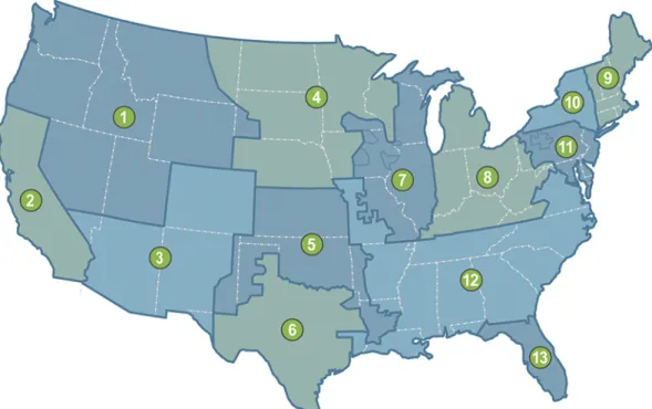
Region 1 for 2012 ... L-10 Figure M-1. Relationship of response of demand response to price for each sector ... M-5 Figure N-1. Non-PEV hourly demand in 2050, Region 1 (East Central Area Reliability
Coordination Agreement) ... N-1 Figure N-2. Non-PEV hourly demand in 2050, Region 2 (Electric Reliability Council of
Texas) ... N-2 Figure N-3. Non-PEV hourly demand in 2050, Region 3 (Mid-Atlantic Area Council) ... N-2 Figure N-4. Non-PEV hourly demand in 2050, Region 4 (Mid-America Interconnected
Network) ... N-3 Figure N-5. Non-PEV hourly demand in 2050, Region 5 (Mid-Continent Area Power
Pool) ... N-3 Figure N-6. Non-PEV hourly demand in 2050, Region 6 (New York) ... N-4 Figure N-7. Non-PEV hourly demand in 2050, Region 7 (New England) ... N-4 Figure N-8. Non-PEV hourly demand in 2050, Region 8 (Florida Reliability Coordinating
Council)... N-5 Figure N-9. Non-PEV hourly demand in 2050, Region 9 (Southeastern Electric Reliability
Council)... N-5 Figure N-10. Non-PEV hourly demand in 2050, Region 10 (Southwest Power Pool) ... N-6 Figure N-11. Non-PEV hourly demand in 2050, Region 11 (Northwest Power Pool) ... N-6 Figure N-12. Non-PEV hourly demand in 2050, Region 12 (Rocky Mountain Power Area,
Arizona, New Mexico, and Southern Nevada) ... N-7 Figure N-13. Non-PEV hourly demand in 2050, Region 13 (California) ... N-7
List of Tables
Table 15-1. Comparison of Efficiency Assumptions in 2050: High-Demand Baseline versus Low-Demand Baseline... 15-2 Table 15-2. Simple Paybacks for Sectors and Selected Sub-Sectors ... 15-5 Table G-1. Effects of Climate Change on Residential Space Heating in U.S. Energy
Studies ... G-1 Table G-2. Effects of Climate Change on Commercial Space Heating in U.S. Energy
Studies ... G-2 Table G-3. Effects of Climate Change on Residential Space Cooling in U.S. Energy
Studies ... G-3 Table G-4. Effects of Climate Change on Commercial Space Cooling in U.S. Energy
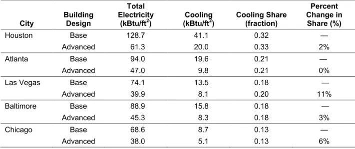
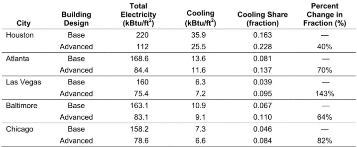
Studies ... G-4 Table H-1. Summary of Results from Efficiency Potential Meta-Analysis ... H-5 Table H-2. Relative Changes in Cooling Electricity Share for Advanced Medium Office
Building... H-14 Table H-3. Relative Changes in Cooling Electricity Share for Advanced Highway Lodging
Building... H-15 Table H-4. Relative Changes in Cooling Electricity Share for Advanced Retail Building—
Low Plug Load ... H-16 Table H-5. Relative Changes in Cooling Electricity Share for Advanced Retail Building—
High Plug Load ... H-16 Table H-6. Relative Changes in Cooling Electricity Share for Advanced Grocery
Building... H-18 Table H-7. Development of Cooling Share Adjustment Factor for Commercial
Buildings ... H-20 Table H-8. Development of Cooling Share Adjustment Factor for Residential
Buildings ... H-22 Table H-9. National Energy Modeling System End Uses by Sector ... H-24 Table I-1. Electricity Purchases Annual Growth Rates for Each Industrial Sector,
2020–2030... I-3 Table I-2. Reduction in Low-Demand Purchased Electricity per Shipment Values versus
High Demand ... I-5 Table I-3. Load Factors by Sector and Region, 2008 ... I-6 Table I-4. Load Duration Curve Definition Factors for East Central Area Reliability
Coordination Agreement, 2050 ... I-7 Table I-5. East Central Area Reliability Coordination Agreement Average Loads for
High-Demand Baseline 2050 for Regional Energy Deployment System Time Slices ... I-11 Table K-1. Ten States with Least and Greatest Percent Change in Population,
2010–2050... K-4 Table K-2. Market Penetration Model Parameter Values for plug-in electric vehicles ... K-6 Table K-3. United States and Top 15 States with Stock Distribution of plug-in electric
vehicles (millions) ... K-7 Table L-1. Segments of Supply Curves for Thermal Energy Storage ... L-1 Table L-2. Peak Hour, Average Hourly Cooling Load, and Thermal Energy Storage Capacity
Table L-3. Estimated Costs for Chilled Water Thermal Energy Storage per Kilowatt
Shifted ... L-5 Table L-4. Cost Assumptions for Thermal Energy Storage, by Step—North American
Electric Reliability Corporation Region 1 ... L-6 Table L-5. Limiting Fractions of Total Cooling Demand, by Step—North American Electric
Reliability Corporation Region 1 ... L-9 Table M-1. Summary of FERC Estimated Demand Response Potential Savings (MW) in
2019 for East North Central Region ... M-2 Table M-2. Census and Electric Power Research Institute Region Assignments to North
American Electric Reliability Corporation Regions ... M-3 Table M-3. Shift of Market Penetration Categories for Demand Response ... M-4
Introduction
The Renewable Electricity Futures Study (RE Futures) is an initial investigation of the extent to which renewable energy supply can meet the electricity demands of the contiguous United States1 over the next several decades. This study includes geographic and electric system operation resolution that is unprecedented for long-term studies of the U.S. electric sector. The RE Futures study is documented in four volumes: Volume 1 describes the analysis approach and models along with the key results and insights from the analysis; Volume 2 documents in detail the renewable generation and storage technologies included in the study; Volume 4 documents the operational and institutional challenges of integrating high levels of renewable energy into the electric grid; this Volume—Volume 3—details the end-use electricity demand and efficiency assumptions.
The projection of electricity demand is an important consideration in determining the extent to which a predominantly renewable electricity future is feasible. Any scenario regarding future electricity use must consider many factors, including technological, sociological, demographic, political, and economic changes (e.g., the introduction of new energy-using devices; gains in energy efficiency and process improvements; changes in energy prices, income, and user behavior; population growth; and the potential for carbon mitigation).
In projecting electricity use, the primary historical drivers for electricity demand (population growth and economic growth) are taken into account along with other emerging trends, including the green building and supply chain1 movements, carbon mitigation, policies and legislation dealing with codes and standards, research and development in energy efficiency, and foreign competition for manufacturing. For the RE Futures, two demand projections were developed to represent probable higher and lower electricity trajectories—hereafter referred to as the High-Demand Baseline and the Low-High-Demand Baseline. The two electricity demand trajectories used in RE Futures rely on the same assumptions for population and economic growth, so the differences stem from the assumptions regarding other trends.
The emerging trends noted above that lead to increased efficiency motivate the Low-Demand Baseline. Based on these, a scenario was developed in which there is an approximately 30% reduction in overall electricity intensity2 within the buildings sector, a 50% reduction in
industrial electricity intensity, and electrification of approximately 40% of the light-duty vehicle stock by 2050.
The High-Demand Baseline is a business-as-usual scenario that assumes trends for the residential, commercial, and industrial sectors as forecast to 2030 by the Energy Information Administration (EIA) in its Annual Energy Outlook (AEO) (EIA 2009d). Because AEO 2009 contained only a forecast through 2030, RE Futures extended the AEO trends out to 2050. Under this scenario, the overall electricity intensity within the buildings sector remains relatively unchanged from 2010 to 2050, and the industrial sector electricity intensity declines by approximately 35% during the RE Futures period (2010–2050).
1 As public awareness of environmental issues grows, consumers and retailers are becoming more interested in the
energy and environmental impacts of the entire manufacturing process, with some retailers (most notably WalMart) issuing green supply chain requirements.
Chapter 13. General Assumptions
Although there is a growing body of literature dedicated to factors affecting energy demand, including behavioral influences, climate change, and new technologies and materials, the explicit inclusion of the potential impacts arising from these influences is beyond the scope of RE
Futures. RE Futures relied on readily available data and projections to the extent possible, and attempted to stay within reasonable bounds established by recent literature. RE Futures was further constrained by the modeling requirement for hourly load projections through the study period. This required the conversion of the estimated projections of electricity consumption into regional hourly load profiles. Although studies projecting potential energy consumption futures are plentiful, studies that tie those consumption futures to hourly loads are not readily available. The basis for the scenarios presented was predominantly drawn from EIA’s AEO for 2009 (industrial sector) and 2010 (buildings sector), which assumed that the major long-term drivers of energy demand—Gross Domestic Product and population—grow at 2.4%/yr and 0.9%/yr, respectively, over the period 2008–2035.3
The fuel prices assumed by the AEO were also taken into consideration in developing the scenarios because increasing natural gas prices might lead consumers to change out their natural gas heating equipment to equipment fueled by electricity, for example; however, given recent prospects to exploit shale gas deposits, the AEO forecast for natural gas prices was believed to be too high. As such, RE Futures did not assume more fuel switching from natural gas to electric devices for space and water heating than was already assumed in the AEO 2010 Reference Case (EIA 2010). Given the extreme difficulty of capturing carbon emissions arising from distributed use of fossil energy in the buildings sector, however, use of decarbonized electricity to provide space and water heating may be an important means for reducing carbon emissions in the future. Recent work for the European Union (European Climate Foundation 2010) projected greater electrification within the buildings sector; as a consequence, forecasted efficiency gains were offset by new electrical demands from transportation and space and water heating. While the total electrical demand for RE Futures would be represented by the High-Demand Baseline in such a case, the underlying load shapes would not capture the resulting hourly and seasonal changes.
Electricity prices also have an impact on the demand for electricity. However, because the demand profiles are provided as exogenous inputs to the models used in RE Futures, the
potential impacts on demand due to changes in electricity prices caused by the various scenarios were not considered in developing the demand projections. The interactions that impact
electricity prices between electricity supply and demand are complex and beyond the scope of RE Futures. The efficiency gains are assumed to be cost-effective using today’s electricity prices and the current AEO forecasts for electricity prices.
Within the commercial sector, two additional trends underlie the AEO projections. First, the growth in disposable income increases the demand for services that depend on computers and other electronic equipment. Also, the growing share of the population over age 65 increases the
demand for health care and assisted-living facilities and the demand for electricity to power medical and monitoring equipment at those facilities. Trends in the residential sector include population migration into the South and the West;4 the conversion of older homes from room air conditioning to central air conditioning; and the growth in the use of “other” appliances,
including large-screen televisions and computers. Within the industrial sector, the AEO projects that energy-intensive manufacturing industries will show slow growth due to increased foreign competition. Additionally, an increase in the use of biofuels in the transportation sector is expected to lead to an increase in the conversion of biomass to fuels such as ethanol, diesel, and jet fuel. This process creates heat, which can be used for industrial on-site generation.
Chapter 14. Potential Impact of Carbon Mitigation Measures and
Climate Change on Electricity Demand
There is currently much discussion about climate change, emissions, and carbon mitigation measures. Potential policies, legislation, and regulation can logically be expected to have an impact on the way in which energy is generated, delivered, and used, whether by specific controls or through pricing incentives or disincentives. The same drivers that might push the United States toward more renewable generation of electricity would also be expected to lead to increased energy efficiency—that is, a drive to use less energy to yield the same level of service. These drivers act in opposition to other trends, such as population growth and the development of new electricity-using devices. Climate change influences another aspect of the energy use picture because heating and cooling loads are highly dependent upon outside temperature. Although a carbon mitigation policy was not explicitly assumed for RE Futures, implementation of a carbon mitigation policy would have an impact on electricity demand. Depending on how such a policy might be implemented, one potential outcome is higher prices for fossil energy, which could lead to fuel switching in end uses such as space and water heating. The Electric Power Research Institute (EPRI) (2009), the National Academy of Sciences (NAS et al. 2009), and the Union of Concerned Scientists (Cleetus et al. 2009) all use reference cases from recent editions of EIA’s AEO. The extent to which fuel switching occurs in these projections is largely due to how EIA models fuel choice in its existing residential and commercial building models. In general, some amount of fuel switching (in the sense of the predicted fuel shares of space and water heating in new buildings) occurs as a function of projected fuel prices and the menu of available energy efficiency technologies for these end uses. With regard to the energy efficiency scenarios undertaken by these studies, none of them makes any explicit assumptions about any fuel switching that would alter the future evolution of electricity growth in buildings.5 One of the results of a greater percentage of renewable generation is that the generation sector would reduce its use of natural gas in the longer term. Currently, electricity generation is responsible for approximately one-third of the U.S. demand for natural gas;6 reduced demand could potentially lower natural gas prices, countering to some extent the price increases brought about by carbon policies.
Just as climate mitigation policies may impact electricity demand, climate change would also be expected to impact both energy supply and energy demand, and numerous studies have been conducted to determine the potential impacts of climate change on the U.S. (and world) energy picture (e.g., Scott and Huang 2007; Huang 2006; Mansur et al. 2005; Scott et al. 2005). Although these studies present varying estimates of the impact on energy demand within the United States,7 they are in general agreement that overall heating consumption is expected to
5 The NAS study is based in part on the Clean Energy Futures report (Interlaboratory Working Group 2000), an
earlier study that assumed some fuel switching in the direction of increased gas use relative to electricity. The NAS study indicates that the estimates of this impact were eliminated in the more recent assessment of future electricity consumption.
6 U.S. Department of Energy, Energy Information Administration, Annual Energy Outlook 2010, Table A.2, http://www.eia.doe.gov/oiaf/aeo/pdf/appa.pdf (EIA 2010)
7 These estimates depend on assumed change in temperature and year, as well as model differences, regions, and
decrease due to climate change (ranging from -3% to -35% by 2050), while overall cooling consumption could increase, ranging from 4% to 90% by 2050 (see Appendix G for
comparisons). For RE Futures, climate change was not explicitly addressed because the overall impacts are subject to a number of assumptions, including temperature change and time frame, that are beyond the scope of RE Futures. Generally, if climate change and climate mitigation policies were to be taken into account, the demand profiles presented here would most likely be underestimating cooling and overestimating heating (although the lower heating demand may cause more switching into electricity, e.g. heat pumps that would offset some of the direct effects of higher temperatures).
Chapter 15. Resulting Scenarios
RE Futures selected two energy demand scenarios to represent reasonable bounds for the
electricity generation requirements through 2050. These two scenarios represent a “higher” level of demand (the High-Demand Baseline) and a “lower” level of demand (the Low-Demand Baseline). Developing scenarios of energy use 40 years into the future is challenging, and the analysis is further complicated by the requirement for detailed hourly system load shapes by region, which are needed for the modeling effort.
The High-Demand Baseline represents a business-as-usual case that assumed that trends within the residential, commercial, industrial, and transportation sectors recently forecast by the EIA (EIA 2009d and EIA 2010) to 2030 continue through 2050.8 This scenario assumed no radical changes in available technologies or consumer behavior, although current technologies will evolve in terms of cost and efficiency. No new regulations or laws not already enacted are included in an AEO Reference Case, and beyond its 2030 horizon, a simple extrapolation is made to 2050. The AEO Reference Case was chosen to represent a higher demand trajectory because it does not include planned equipment and appliance standards or proposed energy code changes, which are expected to lower demand.
The Low-Demand Baseline assumed a moderately high level of energy efficiency within the buildings and industrial sectors. The Low-Demand Baseline assumed that approximately 40% of the light-duty vehicle stock becomes electrified by 2050. In the buildings sector, the efficiency improvements necessary to achieve ultra-high-efficiency buildings are estimated,9 while in the industrial sector, estimated responses to carbon restrictions, based on the Waxman-Markey cap and trade provisions, are applied.
The electricity demand forecasts for buildings, industry, and transportation represent sales trajectories. Transmission and distribution losses are not considered as part of these on-site electricity projections. The electricity sector is expected to deliver these energy quantities according to the timing and distribution specified by the corresponding load shapes used in the models.
Table 15-1 compares the two scenarios and their underlying assumptions, which are discussed more fully in the following sections.
8 Both the 2009 AEO Reference Case (April Stimulus version) (EIA 2009d)and the 2010 AEO Reference Case
(EIA 2010) were used. The opportunity to use the 2010 AEO for the buildings sectors became available later in the Renewable Electricity Futures Study period; compared to the 2009 AEO Reference Case, the 2010 AEO Reference Case shows a small reduction in both residential (1.5%) and commercial (3.2%) electricity use in 2030. For the commercial sector, the somewhat greater reduction appears to be related to the availability and adoption of more efficient lighting, refrigeration, and computer technologies.
Table 15-1. Comparison of Efficiency Assumptions in 2050: High-Demand Baseline versus Low-Demand Baseline
Sector High-Demand Baseline Low-Demand Baseline
Residential 2% decline in intensity over 2010 levels 30% decline in intensity over 2010 levels Commercial 5% increase in intensity over 2010 levels 32% decline in intensity over 2010 levels Industrial 35% decline in intensity over 2010 levels 50% decline in intensity over 2010 levels Transportation <3% plug-in hybrid electric vehicle (PHEV)
penetration 40% of vehicle sales are plug-in electric vehicles (PEVs)
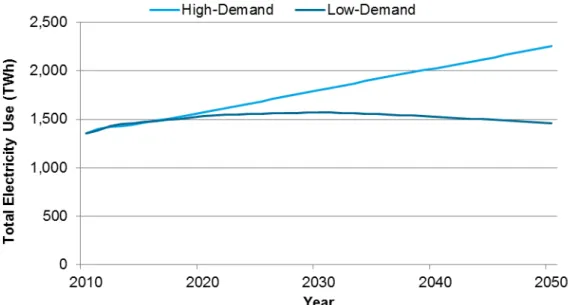
Figure 15-1 illustrates the resulting demand trajectory for the Low-Demand and High-Demand Baselines through 2050. For comparison, the EIA analysis (EIA 2009b)10 of the American Clean Energy and Security Act of 2009 (the Waxman-Markey Climate Bill from 2009)11 is included, using the 2025–2030 trend to extend the analysis to 2050.
Figure 15-1. Total electricity demand, 2010–2050
10 For its analysis, EIA ran a number of cases for the bill. The “EIA Waxman-Markey Analysis” line in this chart
Figure 15-2 illustrates the electricity consumption by sector for the High-Demand Baseline and the Low-Demand Baseline. For context, Figure 15-3 contains the historical energy use by sector.12
Figure 15-2. Total electricity demand, 2010–2050: High Demand (high) and Low Demand (low) by sector
Figure 15-3. Historical and projected electricity demand assumptions in low-demand and high-demand scenarios
12 The leveling of the industrial sector electricity demand is due in part to reduced production within the
manufacturing sector. Appendix I contains a breakdown of the changes in the industrial sector due to energy efficiency versus declining production for the period 2010–2030.
Unlike the renewable technologies explored in RE Futures, the reductions in consumption have been generated without explicitly considering the investment needed to realize these gains. Terms such as cost-effective or cost-competitive are often used in discussing energy efficiency measures. These generally mean that the efficiency measures cost less or about the same as their less efficient counterparts once the various costs (e.g., energy, operation and maintenance, capital) over the lifetime of the measure are considered. Although these investment costs are not considered here, findings from other studies are presented to illustrate the approximate cost of efficiency gains to provide some perspective.
The National Academy of Sciences (NAS et al. 2009) reported conservation supply curves for energy efficiency in the buildings sector that were originally developed by Lawrence Berkeley National Laboratory (Brown et al. 2008). These supply curves indicated that energy savings of 30%–35% could be achieved over Brown et al.’s reported reference case at a cost less than the 2007 retail cost of energy. For electricity, the conserved cost of energy was found to range from less than 1 cent per kWh to about 8 cents per kWh, with an average conserved cost of energy of 2.7 cents per kWh. Brown et al. (2008) calculated that the cumulative capital investment13
required between 2010 and 2030 to achieve their level of electricity savings14 was approximately $299 billion.15 Combined with average annual electricity bill savings of $128 billion in 2030, electricity efficiency measures, on average, had a payback of 2.3 years. Additionally, NAS et al. (2009) reported that energy savings of 14%–22% could be cost-effectively achieved by 2020 within the industrial sector. Within the National Academy of Sciences study, cost-effectiveness was defined as an internal rate of return of at least 10% or exceeding a company’s cost of capital by that company’s defined risk premium; however, no conserved cost of energy was specifically reported for the industrial sector.
In another study, McKinsey and Company (Granade et al. 2009) calculated the cost-effective energy efficiency potential in the residential, commercial, and industrial sectors.16 Granade et al. (2009) calculated the present value of investment costs and annual energy savings for each sector, as well as a set of sub-sectors. Table 15-2 contains the simple paybacks calculated for selected categories.
13 The cumulative capital investment is the reported capital investment as an incremental investment, including only
costs above those incurred in the reference case. It includes the full “add-on” cost for new measures or equipment (such as additional insulation) as well as the incremental cost of the efficient technology compared with the cost of the conventional technology equivalent (e.g., the difference in price between a highly efficient heat pump and an electric air conditioner/furnace combination).
14 For reference, Brown et al. (2008) estimated electricity savings within the buildings sector of about 1,270 TWh in
2030; the Low-Demand Baselinefor the Renewable Electricity Futures Study estimated electricity savings in the buildings sector of approximately 410 TWh in 2030 and 1,350 TWh in 2050.
15 All dollar amounts presented in this report are presented in 2009 dollars unless noted otherwise; all dollar amounts
presented in this report are presented in U.S. dollars unless otherwise noted.
16 McKinsey and Company (Granade et al. 2009) estimated the overall energy efficiency potential, defined as net
present value positive. Total energy savings of 5.45 quadrillion Btu (buildings) and 3.65 quadrillion Btu (industrial) in 2020 were calculated, including 900 TWh of electricity savings (buildings) and 190 TWh of electricity savings
Table 15-2. Simple Paybacks for Sectors and Selected Sub-Sectorsa
Sector Simple Payback (years)
Residential 5.617 Existing Homes 9.5 New Homes 4.0 Commercial 3.418 Existing Private 6.6 New Private 3.8 Government 5.2 Industrial 2.4
Energy Support Systems 2.0 Energy-Intensive Processes 2.7 Non-Energy-Intensive Processes 2.5
a Granade et al. 2009
Another cost estimate can be drawn from Lazard (2009), which reports a levelized cost of energy for energy efficiency measures to range from 0 cents/kWh to 5 cents/kWh, based on utility costs as reported in the joint U.S. Environmental Protection Agency and U.S. Department of Energy (DOE) National Action Plan for Energy Efficiency Report (DOE/ 2006).
17 Includes investment and annual energy savings associated with electrical devices and small appliances, and
lighting and major appliances (Granade et al. 2009)
18 Includes investment and annual energy savings associated with community infrastructure and office and
Chapter 16. Building Sector Electricity Demand
The buildings sector dominates overall electricity consumption, representing almost 78% of the 2030 total in the AEO Reference Case.19 Additionally, building electrical end uses are highly heterogeneous and changing over time.
16.1 Low-Demand Baseline
Within the buildings sector, trends that can be expected to influence future electricity use include the “green” building movement, more stringent building codes, more stringent appliance and equipment standards, and research by the DOE and others to develop ultra-efficient buildings. Ultra-efficient buildings are designed and operated to generate as much on-site power as the energy they consume.20 Some of the approaches to achieving this ambitious goal include developing and applying very high-efficiency technologies, finding ways to reduce the cost of energy-efficient technologies that have already been developed, and implementing cost-effective technologies that are already available.
Because the focus of RE Futures was on the generation of electricity, the lower-demand baseline was developed using a more generic, energy-intensity projection, rather than attempting to build a projection up from the various technologies and practices available within each of the end uses. Although a certain level of energy efficiency gains is possible through the normal adoption of new energy-efficient practices and technologies, the larger gains here implicitly require more active policy and behavioral change to come to fruition. The efficiency gains within the Low-Demand Baseline are assumed to be feasible by sustained efforts on the part of government, businesses, and households, and to be cost-effective without major increases in electricity prices as a driver. It is implicit to efficiency gains that the measures are properly installed, operated, and maintained as intended, and that the resulting savings are not used to increase the level of service (e.g., permanently adjusting the thermostat).21
Although a detailed analysis of policy changes remains to be examined, potential policy changes could include increased code adoption and enforcement; financial incentives such as tax credits, energy efficient mortgages, rebates, and coupons; broadening rating and labeling efforts; and encouragement of volume purchase programs. Behavioral changes could include users using technologies such as controls and sensors as they were intended, a greater focus on continuous building commissioning, and acting on available information on energy use. Other changes might include an increased focus on building commissioning so that buildings are built and commissioned as designed; more integration between the financial, construction, and associated industries to better enable the deployment of highly efficient buildings; and deployment of smart meters to provide users with a better understanding of their energy consumption.
19 EIA AEO (EIA 2010) Table 2.
20 Generally, ultra-efficient buildings are assumed to reduce their energy requirements by up to 70%, with the
remainder of the building load met by local generation sources, such as photovoltaics. For RE Futures, only the efficiency improvements were considered as input to the end-use electricity demand.
16.1.1 New Building Energy Intensity
The Low-Demand Baseline for RE Futures was based on the energy efficiency vision of DOE’s ultra-efficient building programs. Consideration of what level of energy consumption intensity must be achieved to reach ultra-high efficiency motivates the overall approach to projecting future energy demands for the residential and commercial buildings. The electricity demand forecast for residential and commercial buildings under the Low-Demand Baseline assumes a larger number of buildings to be capable of ultra-high efficiency. Due to the inability to predict which technology and end-use consumption areas are most likely to show the greatest
improvements, the Low-Demand Baseline focused only on the broadest measure of energy intensity: energy use per square foot (or per household) at the whole-building level. Accordingly, the basic assumption for new buildings is that the average energy intensity in 2050 will be 60% below that of new buildings being built today.22 The factors underlying this reduction include increased energy code stringency, the continued development and implementation of federal energy efficiency standards for equipment and appliances, and research and development efforts directed at both the component and system (or whole-building) level. This reduction is also assumed to occur along an exponentially declining path. Thus, absolute reductions in energy intensity are assumed to be greater in the immediate future than several decades from now. Additional detail on the approach and assumptions can be found in Appendix H.
16.1.2 Existing Building Energy Intensity
Due to the cost to substantially change the building envelope and the heating and cooling system, the potential for large efficiency increases for existing buildings is much lower than that for new buildings. Moreover, the addition of electrical services in older buildings (e.g., air conditioning) tends to increase electricity consumption. However, both research and development
improvements and federal energy efficiency standards for equipment and appliances will contribute to a reduction in electricity use. For the Low-Demand Baseline, intensity in existing residential buildings (e.g., pre-2010 homes still in the stock in 2050) was assumed to decline by 30% by 2050. For commercial buildings, the assumed decline by 2050 is somewhat greater at 40%. The larger decline for commercial buildings reflects an assumption that the amount of miscellaneous electrical uses in commercial buildings will be more amenable to reductions from policy and new technology than those in the residential sector. Additional detail on the approach and assumptions can be found in Appendix H.
16.1.3 Retrofits and Renovations
For a study with a long-term time horizon, one cannot assume that the intensity of buildings built today and in the near future will remain constant through 2050. Many ultra-high efficiency technologies introduced in the latter years (2030–2050) will be adopted, through retrofits and renovations, in buildings built over the next 20 years. As a means of accounting for that phenomenon, the Low-Demand Baseline assumed that buildings (both residential and commercial) built over the next 20 years (2010–2030) will be retrofitted (or renovated) with
22 Best practices guides and case studies that illustrate pathways to achieving 15%–40% whole-building energy
savings for various residential climate zones are available via DOE’s Building America website
(http://www1.eere.energy.gov/buildings/building_america/climate_specific_publications.html). Design guides and strategies containing pathways to achieving 30%–50% whole-building energy savings for selected building types within the commercial sector are available through the U.S. Department of Energy’s Commercial Building Initiative website (http://www1.eere.energy.gov/buildings/commercial_initiative/guides.html).
more efficient equipment in the subsequent 20 years (2030–2050). Operationally, this
assumption is implemented as a 15% reduction in the electricity intensity for housing units and a 20% reduction in commercial buildings starting in 2031. In other words, residential and
commercial buildings built between 2010 and 2030 are “revisited” in the analysis 20 years later (e.g., buildings built in 2011 are revisited in 2031; buildings built in 2012 are revisited in 2032, and so on, through 2050), with the intensity reduction applied in the out years to account for improvements in building and equipment practices.
16.2 High-Demand Baseline
The High-Demand Baseline for the residential and commercial sectors uses the AEO Reference Case (EIA 2010), as mentioned earlier. The AEO assumed that total electricity consumption grows by 0.9%/yr from 2007 to 2030. Commercial growth is approximately 1.4%/yr (with commercial electricity intensity in kilowatt-hours per square foot increasing by 0.1%/yr), and residential growth is approximately 0.8%/yr (with electricity use per household declining at an average annual rate of 0.2%/yr). Documentation of the assumptions is found in the AEO 2009 and AEO 2010 and supporting materials (EIA 2009a; EIA 2009d; EIA 2010).
16.3 Comparison of Projected Energy Intensities
To provide some context for the both the High-Demand and Low-Demand Baselines, the energy intensities have been compared to other studies. The comparison studies are from the Union of Concerned Scientists (Cleetus et al. 2009), University of California-Davis (McCarthy et al. 2008), EPRI (2009), EIA’s analysis of Waxman-Markey (EIA 2009b), and NAS et al. (2009). To maintain the focus on potential energy efficiency improvement, the comparisons have been made in terms of energy intensities. Consistent with EIA’s AEO, the intensity for the residential sector is in terms of electricity use per household; for the commercial sector, energy use per square foot of floor space is employed as the intensity measure. For comparison purposes, the intensities were converted to index numbers normalized to be 1.0 in 2010.
Figure 16-1 shows the projected intensities for the residential sector, and Figure 16-2 shows the scenarios from the same studies for the commercial sector. Within the residential sector, the High-Demand Baseline shows the least decline in intensity to the year 2030, while commercial sector electricity under this scenario is expected to increase through 2030. The light blue squares connected by the solid line in both figures depict the high-efficiency scenario (Low-Demand Baseline) developed for RE Futures. As shown in Figures 16-1 and 16-2, this scenario falls within the range of intensity forecasts drawn from other studies. Although not included in the figures, McKinsey and Company (Granade et al. 2009) conducted another recent study of cost-effective energy efficiency potential in the United States. When converted to an index basis, the implied intensity indexes (2020 relative to a 2010 base) for the residential and commercial sectors are 0.71 and 0.73, respectively. These values are substantially lower than those shown for 2020; however, due to the shorter time frame and greater emphasis on cost-effective potential compared to other studies, these values are not shown in either figure.
Figure 16-1. Residential electricity intensities from six studies, including RE Futures
Figure 16-2. Commercial electricity intensities from six studies, including RE Futures
Sources: EIA 2009b, EPRI 2009, Cleetus et al. 2009, McCarthy et al. 2008, NAS et al. 2009
Chapter 17. Industrial Demands and Energy Efficiency
The industrial sector accounts for approximately 27% of total electricity demand,23 with more than 50% used to power electric motors (representing the single largest end use of electricity in the United States).24 Within the industrial sector, the chemicals and primary metals industries consume the most electricity, representing approximately 35% of electrical consumption.25 The sector’s electricity use will be impacted by increases in the efficiency of motor drive systems and other processes, a slower growth rate of the more energy-intensive manufacturing industries, and a shift toward green supply chains. The sector is also affected by foreign competition.
In projecting industrial loads over the next 40 years, there are a number of unknowns. Industrial demands are more difficult to project due to the wider variation in the industrial sector makeup over time, as well as large differences in energy intensity across various industries. The extent of changes from the energy sector that would feed back in to the industrial sector based on different renewable energy scenarios further complicates the task of projecting loads and would ideally require iteration. Because RE Futures is a renewable energy study and not an industrial demand study, an approximation of the projected industrial demands was deemed sufficient.
A more detailed analysis of the consequences of some factors of the renewable energy scenarios, such as construction of renewable energy technologies and electric vehicle batteries, may result in increased load forecasts for some industrial sub-sectors, while other sectors, such as oil refining, may see countervailing changes. Possible changes in onshore versus outsourcing of manufacturing are also a large unknown and are beyond the scope of RE Futures. In addition, climate change, new processes for existing products, and new products altogether further magnify the uncertainty regarding future industrial loads.
17.1 Low-Demand Baseline
The Low-Demand Baseline industrial demand trajectory is derived in a quite different manner than that used for the buildings sector. It was based on the EIA’s HR2454Cap National Energy Modeling System (NEMS) Case,26 which, as its name suggests, includes a carbon cap and trade policy roughly equivalent to the provisions of the Waxman-Markey Climate Bill from 2009. Given that this case would evoke a significant efficiency boost (ranging from 6% to 69% in 2050, depending on the specific industrial sector), RE Futures believed its consumption level represents a reasonable energy efficiency scenario and adopted it as the Low-Demand Baseline.27 Underlying the Low-Demand Baseline are EIA’s assumptions that further standards for
industrial energy efficiency will be established, an awards program for increasing efficiency in the thermal electricity generation process will be created, and the waste-to-heat energy incentives in the Energy Independence and Security Act of 2007 will be clarified. Overall, the changes in
23 EIA AEO (EIA 2010), Table 2 24 EIA 2006, Table 5.3
25 EIA 2006, Table 3.1
26 This is the Basic Case described in EIA 2009b.
27 Although RE Futures does not explicitly assume the implementation of any carbon mitigation policy, the
HR2454Cap case was used as the industrial sector input in the high-efficiency case because the resulting industrial loads (and load shapes) were consistent with the higher efficiency targets that characterize the Low-Demand
the Low-Demand Baseline result in an approximately 23% decrease in electricity use compared to the High-Demand Baseline. Appendix I contains additional information about the derivation of the load curves and the implicit energy efficiency gains.
17.2 High-Demand Baseline
The High-Demand Baseline industrial demands provided to the models were based on the electricity sales to industry reported in the 2009 AEO Reference Case (EIA 2009d), with a simple extrapolation beyond 2030 through 2050. The AEO assumed that total electricity
consumption grows by 0.9%/yr from 2007 to 2030, with growth in the industrial sector declining by 0.2%/yr (industrial electricity intensity in terms of consumption per real dollar of shipments declining by 1.3%/yr). Documentation of the assumptions can be found in the AEO 2009 and AEO 2010 and supporting materials (EIA 2009a; EIA 2009d; EIA 2010).
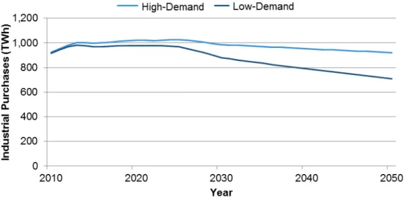
Because the 2009 NEMS version projects energy use only through 2030, the demands for both the High-Demand Baseline and Low-Demand Baseline scenarios were extrapolated to 2050 using the 2020–2030 growth rate (Figure 17-1). Additional calculations explained in Appendix I describe the method used to find the results for each North American Electric Reliability Council region and convert them to hourly profiles.
Figure 17-1. Industrial electricity purchases under the High-Demand Baseline and Low-Demand Baseline
17.3 Comparison of Projected Energy Intensities
As was done for residential and commercial buildings (Section 16.3), a comparison of scenarios for the industrial sector was developed and is shown in Figure 17-2.28 For the industrial sector, the electricity intensity is computed as the electricity consumption per dollar (in real terms) of shipments. For comparison purposes, the intensities were converted to index numbers
normalized to be 1.0 in 2010.
Both the High-Demand Baseline and Low-Demand Baseline are taken from EIA model simulations. The High-Demand Baseline was based on the 2009 AEO Reference Case (EIA 2009d). The Low-Demand Baseline was based on the analysis of the Waxman-Markey Climate Bill from 2009 performed by EIA (EIA 2009b), whose results here have been extrapolated to 2050. Figure 17-2 indicates that the Low-Demand Baseline in this instance is reasonably close to the projections made by both EPRI (2009) and UC–Davis (McCarthy et al. 2008). The Union of Concerned Scientists scenario (Cleetus et al. 2009) is again considerably lower; under its policy and research and development scenario, industrial electricity intensity falls to less than half of its current value by 2030. Although the results are not included in the figures, McKinsey and
Company (Granade et al. 2009) conducted another recent study of efficiency potential in the United States. When converted to an index basis, the implied intensity index (2020 relative to a 2010 base) for the industrial sector is 0.68 in 2020. Because of the shorter time frame and greater emphasis on cost-effective potential compared to other studies, this value is not shown in
Figure 17-2.
Figure 17-2. Industrial electricity intensities from five studies, including RE Futures
Sources: EIA 2009b, EPRI 2009, Cleetus et al. 2009, McCarthy et al. 2008, NAS et al. 2009
Appendix G provides additional detail regarding the comparison studies.
17.4 Combined Cooling, Heating, and Power within the Industrial Sector
The industrial sector can generate some of its own power needs, either through dedicated electricity plants or through combined cooling, heating, and power plants. Some of this power generated may also be sold to the electric sector for sale to other sectors. Total industrial electricity demand is the sum of purchased electricity and electricity generated less electricity sold to the grid. For RE Futures, the amount of cooling, heating, and power embedded within the High-Demand Baseline and the Low-Demand Baseline was determined, as discussed in
Appendix J. No additional modifications were made to either increase or decrease the amount of cooling, heating, and power within the industrial sector.
Chapter 18. Transportation Demands
Although electricity use in the transportation sector is currently negligible (less than 0.2%),29 plug-in electric vehicles (PEVs) offer the opportunity for the transportation sector to significantly reduce petroleum consumption through electrification. Light-duty vehicles currently use more than 60% of the energy consumed in transportation, making them the primary focus of an electrification effort.30 Medium- and heavy-duty vehicles are the next largest segment (approximately 20%) and, while some portion of these could likely be electrified, it is quite difficult to compete with diesel powertrains in these applications. The likely load shape of medium- to heavy-duty vehicles is also less certain, making the development and incorporation of their associated load shapes into the models difficult. Therefore, RE Futures concentrated the transportation electrification effort in the light-duty vehicle market. Additionally, hybrid PEVs may have moderately sized energy storage systems and combustion engines that operate over a limited range under battery power while retaining the range capability of conventional
combustion-engine vehicles. Other PEVs may be entirely battery dependent and provide
complete petroleum displacement for specific vehicle sectors—several manufacturers are slated to introduce these types of vehicles to the market over the next several years. Based on past technology markets, maturity would likely occur within several decades from introduction. The introduction of PEVs also creates new flexible loads that can be integrated into utility operations with a high penetration of renewables to achieve a long-term strategy of creating a more sustainable transportation system.31 RE Futures developed energy system load
characteristic forecasts on a regional basis during the study period. The work builds upon past travel survey data analyses, regional population forecasts, and charge management scenarios.
18.1 Low-Demand Baseline
Results were generated for 3,109 counties and were consolidated into 134 balancing areas (BAs) for use in regional generation planning analysis tools. PEV aggregate load profiles from previous work were combined with vehicle population data to generate hourly loads on a regional basis. A transition from consumer-controlled charging toward utility-controlled charging was assumed such that by 2050, approximately 45% of the transportation electricity demands could be optimally managed from the utility perspective. No other literature has addressed the potential flexibility in energy delivery to electric vehicles in connection with a regional power delivery study. This electrified transportation analysis resulted in an estimate for both the flexible load and fixed load shapes on a regional basis.
As input to RE Futures, hourly PEV load and energy demand profiles for the fleet of PEVs by region over time were developed. The approach was as follows:
1. Use population growth forecasts and historical vehicle ownership trends to estimate vehicle population by region
29 EIA AEO (EIA 2010), Table 2
2. Use a market evolution model to estimate the fraction of vehicles that will be PEVs throughout the study period
3. Develop a vehicle fleet energy demand profile based on those from past studies that transitions from market introduction with no utility control to one in which the utility is able to manage a portion of the vehicle load.
Simplifying assumptions, detailed in Appendix K, were made to constrain the study scope. A PEV market growth and saturation model was used with the motor vehicle estimates to determine the number of PEVs likely to be in use on a county level over the period discussed in RE Futures. The market model represents a slow ramp toward consistent market growth and a final tapering of growth to saturation. PEV sales saturates at a 50% market share after about 50 years (equivalent to approximately 40% of the total stock by 2050). A comparison of the sales rate and vehicle stock is shown in Figure 18-1. The rates in this scenario are consistent with results recently developed by Lin and Greene (2010).
Additional calculations to convert the demand to hourly profiles are explained in Appendix K. This appendix also discusses the development and application of three charging profiles:
• A No Utility Control profile in which the consumer is allowed to plug in and charge as soon as the vehicle ends the last trip for the day
• An Opportunity profile in which the charging infrastructure is prevalent and the consumer will choose to plug in any time the vehicle is parked
• A Valley Fill/Managed profile that allows utilities to choose the charging time for vehicles
The energy demands of the Valley Fill/Managed scenario are assumed to grow to become a flexible load that can be managed by the utility to improve renewable generation asset
utilization. By 2050, 45% of the total vehicle energy demand of 350 TWh was under managed control while the remaining 55% was a fixed load to be planned for and met by utility assets. The hourly load profile of the fixed transportation energy demand also shifted over the time period from No Utility Control toward Opportunity Charging.
Figure 18-1. Technology market penetration scenarios
18.2 High-Demand Baseline
For the High-Demand Baseline, the 2009 AEO Reference Case (EIA 2009d) was used to represent the transportation sector. Within the 2009 AEO Reference Case, PHEVs with a 10- to 40-mile all-electric range represented less than 3% of vehicle sales by 2030 (EIA 2009d), and overall electricity use by the transportation sector remains less than 1% by 2030.
18.3 Comparison to Other Studies
Many analyses have been conducted and papers published that include PEV market projections. EPRI and the Natural Resources Defense Council collaborated on a foundational study
highlighting the nationwide greenhouse gas and pollutant emissions impacts of PEVs on the U.S. electrical grid on a regional basis (EPRI 2007). The fleet makeup assumed approximately 40% PEVs by 2030 and 60% by 2050. An aggregate hourly load profile was assumed in which 74% of the energy was delivered during the off-peak period and 26% during the daytime. Both the Pacific Northwest National Laboratory and the Oak Ridge National Laboratory have assessed regional PEV penetrations and future load characteristics. The Pacific Northwest National Laboratory study (Scott et al. 2007) considered the situation in which all electric vehicle loads could be managed and fit into the low points of the daily utility load curve. The Oak Ridge National Laboratory study (Hadley and Tsvetkova 2008) considered a variety of charge levels and loading scenarios to understand the regional capacity and emissions impacts of the various scenarios.
Chapter 19. Hourly Electricity Demand for 2050
The potential for renewable electricity production to meet a large portion of future electricity demand depends not only on the magnitude of that demand but also on its variability regionally, seasonally, and diurnally; therefore, RE Futures focuses on load shapes. A central challenge for RE Futures was to convert the energy forecasts to the 13 regional hourly system load shapes required for the models.32 Within the EIA’s NEMS residential and commercial buildings modules, energy consumption by end use is forecast individually and regionally (EIA 2009c). These annual energy estimates are then attached to corresponding dimensionless load shapes and the results summed up to deliver hourly regional electricity system loads.
Because the High-Demand Baseline is a direct extension of a NEMS run, in this case, the load shapes for all sectors can be derived directly from NEMS (see Figure 19-1). This exercise is described further in Appendix H.
Figure 19-1. High-demand hourly load profile, 2050
32 As described further in Appendix B, both the ReEDS and NEMS models use a set of representative load shapes to