Evaluating the 3G Network Performance by Virtual Testing

125

Evaluating the 3G Network Performance by Virtual Testing

Prabu Jayakumar

and Chiew Foong Kwong

1

INTI International University, Malaysia, Faculty of Engineering and Information Technology 2

INTI International University, Malaysia, Faculty of Engineering and Information Technology Corresponding author: [email protected]

Abstract

The third Generation Universal Mobile Telecommunications System (UMTS) is a well established technology which carries data, voice and multimedia traffics; consequently it means that the vast amount of traffic is handled at Node-B and controlled by Radio Network Controller (RNC) as a major network end interface. Furthermore, the Quality of Service (QoS) is a key concern in wireless networks and it has been achieved by extensive testing of UTRAN; precisely the testing effort is an important requirement of heterogeneous networks. In the beginning stage of the project a detail case study is made about the cellular network planning, designing and optimization techniques, based on the study, a set of problems is observed and a major problem is chosen as a sample for computational experiment. In this project a simulation based approach is used to implement the UTMS network, the virtual field testing concept is to evaluate the performance of UMTS Terrestrial Radio Access Network (UTRAN) terminal and to analyse the Radio Resource Management (RRM) function. There are several factors and criteria that have to be measured and to assess the performance of UMTS network.

The Qualnet software is used for computational experiment; five different types of scenarios are developed to analyse the network behaviours. The scenario-1 is designed to perform the virtual field testing and the following parameters are measured: Energy per bit to noise ratio density (Eb/No), Common Pilot Channel Received Signal Code Power (CPICHRSCP) and User Equipment (UE) layer -2 massages. Beside these measurements sceanrio-2 is developed to optimize the QoS by redefining scenario-1. Additionally Scenario-3, 4 and 5 are designed with different traffic ranges to analyse the capacity and coverage interlink. All the computational experiments are carried using the (Constant Bit Rate) CBR traffic.

Key words: UTRAN, Network Planning, Virtual Testing, Optimisation, Cell Shrinking, Eb/No, CPICHRSCP

1 Background and Motivation

The world’s first cellular system was established in Japan in the year of 1979 and later it was followed by North American in 1983 [6]. Now all over the world we can see different type of cellular system have been installed and the networks are capable of providing wide range of service at high speed. So due to the tremendous growth of mobile communication; the number of subscriber and volume traffic are explosively increased. To strengthen this issue the radio spectrum allocation and the radio resource management should optimum, this can be achieved by executing several types of testing in different phase of the network. Besides, it’s difficult to test the radio network became the architecture is complex and on the other hand it’s problematic to predict the radio network behaviour [4].

The third generation wireless network deployed in this project is referred to UMTS system, which has been implemented through W-CDMA air interface. There are number of transition from 2G to 3G, starting from planning to field validation of the radio terminal. The crucial benefit of the 3G network is they are backward compactable with GSM network and this is achieved because the architecture of the radio terminal in both GSM and UMTS are designed and implemented through Software Defined Radio (SDR). Beyond the architecture and protocol stack of the wireless networks, the QoS (Quality of Service) depends on the cell dimensioning through the air interface, transmission dimensioning, coverage planning, capacity planning and traffic balancing. To maintaining the planned radio coverage optimal usage of the radio resource is very important to deliver the QoS [3]. Today in mobile communication industries 80 percent of the total investment cost is spent for radio access network installation and for optimization to deliver QoS to customers.

Beside the migration of mobile network from second generation to third generation the major change in the architecture is the air interface. The recent survey says that 70 percent of problems are raised by UMTS Terrestrial Radio Access Network (UTRAN). In addition to evaluate the 3G toward 4G forty contributions of approaches and proposals have been presented by equipment manufacturers, operators and research institutes [1]. So to justify the problems raising factor of UTRAN, the virtual testing concept is required to test the behaviour of the network before implementation. Further design, optimize and testing the UTRAN are significant challenging, this are all the important reasons for proposal.

2 Methodology

2.1 Phase of the Project

The phases of this project are classified into five stages. This approach is used to manage the project plan from preliminary concept to an implementation and validation.

 Phase 1: A detail case study of 3G networking architecture is achieved; to understand the network components, functional behaviour of the network.

 Phase 2: Understanding the architecture of qualnet UMTS library model to design and implement the network components accordingly to 3GPP UMTS architecture.

 Phase 3: To evaluate the performance of the 3G radio network, five targeted scenario are planned and designed according qualnet UMTS architectural model.

 Phase 4: The experiments are carryout by deploying the designed scenarios in to the simulation platform to perform network optimization and virtual testing.

 Phase 5: The designed scenarios are executed and the network stability of particular node is tested using the qualnet real-time interface dynamic statistic component.

127

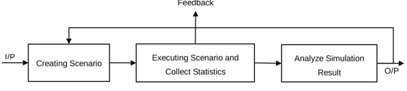
Figure 1: Block Diagram of the Project

2.2 Life Cycle of Simulation

Instead of using the actual network hardware components, a software program is designed to follow the hardware abstract model; using the model the physical network is designed. This kind of simulation experiment is directly closeness of real time network accuracy. The blocks inside the simulation platform denote the features of simulation software, it assists the user to simulate the scenarios and execute. If the output of the system is not valid then the

experiment is

redefined.

Figure 2: Simulation Life Cycle Redefining Experiment

Executing Model

Collecting Statistics

Environment Modelling Device Modelling Traffic Generating

Validation

Reporting Yes No

Simulation Platform

GATHERING 3GPP UMTS ARCHITECTURE PRINCIPLE

GATHERING QUALNET UMTS MODEL PRINCIPLE

PLANNING AND DESIGNING THE NETWORK

VIRTUAL TESTING IS CARRIED OUT USING THE QUALNET DYNAMIC STATIC COMPONENT DESIGNING SCENARIOS

2.3 Simulation Requirement and its Environment

Simulation Environment: In this project the 3G network components and hardware is designed and simulated using the Qualnet software to implement the virtual testing concept. The Qualnet software executed on a standard PC workstations. The scenario components and conditions are defined, like terrain dimensions, channel type, propagation effects, path loss, fading, shadowing wireless subnets and application (traffic). The scenarios are adjusted on observing and analysing the results.

Figure 3: Scenario Based Simulation

Input: Systems designs and description is based on user metrics of interest. Output: Runtime statistics and final statistics using analyzer and output traces.

2.4 Implementing the Simulation

The implementation of the scenario is based on the design. The process of creating scenario is followed by different aspects. The first step is configuring the general properties of the network and it’s a global setting for the particular scenario. Next step is positioning the network elements; configuring the topology using the wireless subnets and configuring all other components are similar. Further on completing the network configuration settings the simulation is executed and the results are generated. The following step involved in creating the scenario,

Figure 4: Process Involved in Creating a Scenario

2.5 Concept of Virtual Testing

The simulation based UTRAN testing approach improves the efficiency of network without performing live testing which is expensive and time consumable task. Virtual testing technique is an emerging methodology which allows test engineers to test the system before real-time implementation through simulation. Furthermore, to carry out the virtual testing “systematic procedure” has to be developed to validate the outcome. In this project the systematic producers and the test strategy are based on Key Performance Indicator (KPI). It is also possible to test the network performance during the runtime using a probing system known as dynamic static which is available in qualnet.

Defining and configuring network parameters

Positioning the node in the terrain Defining network topology structure Configuring wireless environment Configuring network protocol stack Configuring statistic collection Configuring Parallel Simulation Input Analyze Stats

Creating Scenario Executing Scenario and Collect Statistics Analyze Simulation Result Feedback O/P I/P

129

2.6 Methodology Justifying

It is necessary to gathering the concept of 3GPP UMTS network and qualnet UMTS model as it’s the foundation task of this project. The simulation approach is proposed because it would be easier to design the network components, configure, change its subsystem, and to measure its performance. The qualnet simulation software is chosen because it has the UMTS library, which it is designed and tailored according to the 3GPP specification. The experiment planning and network planning are also very important process that is required for sensitivity analyse of wireless network performance. The scenarios are developed and executed according to the art of simulation life cycle. This project consists of five scenarios the first scenario is implemented using random seed component, the second scenario is by redefining the first scenario for optimization using KPI parameters and the scenario three to five is to measure the system capacity by increasing the UE traffic to analyse the interlink between capacity and coverage.

3 Cell Planning and Designing

3.1 Cell Planning

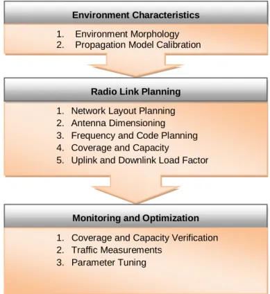
The Cell Planning is generally carried out to provide a quality wireless service. WCDMA air interface has new radio planning techniques. In GSM the capacity and coverage planning are done separately, so a detailed planning phase is required for GSM. While in WCDMA the capacity and coverage are planned simultaneously, the following are planning procedure.

Figure 5: Planning and Designing Process of 3G Cellular Network

3.2 Environment Characteristics

Terrestrial Environment Morphology: The propagation mechanisms are reflection, refraction, scattering and diffraction all these types are extremely based on the terrestrial environment. Therefore, according to the terrestrial sit dimensions, Node-B components have to be design.

Environment Characteristics 1. Environment Morphology 2. Propagation Model Calibration

1. Network Layout Planning 2. Antenna Dimensioning 3. Frequency and Code Planning 4. Coverage and Capacity

5. Uplink and Downlink Load Factor

Monitoring and Optimization 1. Coverage and Capacity Verification 2. Traffic Measurements

3. Parameter Tuning Radio Link Planning

Figure 6: Different Types Environment

Propagation Model Calibration: The propagation model is a statistical formula derived from the empirical measurement data. So according to environment the model is deployed to predict propagation loss but it will do not coincide with real-time radio environments exactly.

3.3 Radio Link Planning

Network Layout Planning: The site survey is carried before implementation of the network, with the help of the surveyed dimension the mathematical design is carried out. To configure the network with core network “Base Station Cell ID” and “Base Station Location Area Code” is assigned.

Antenna Dimension: The antenna is an important component which determines the cell structure. There are different type of antenna used in mobile communication according the coverage issues as well as every antenna has it own radiation pattern relating to its geometry and which directly coupled with the coverage dimension. The transmitting power and the height of the antenna are also taken in to account in planning because it is related to “Cell Coverage Thresholds”. In general sectorised antenna and Omni-directional are used in mobile communication. The Omni-directional antenna is capable of transmits and receives signals at 360 degrees. The sectorised antennas (2 sectorised and 3 sectorised) installed in the BS, which can transmit and receives in certain directions. The 2-sectorised BS antenna is suitable for providing coverage in highways.

Figure 7: (a) Omni Directional Antenna (b) 2 Sectorised Antennas (c) 3 Sectorised Antennas

131

The coverage of BTS naturally differs from theoretical ideal and practical design as below.

Figure 8: (a) Theoretical Coverage (b) Ideal Coverage (c) Practical Coverage

Frequency and Code Planning: In WCDMA all cells uses the same frequency using the different spreading codes (Frequency reuse is n=1), which means the UE simultaneously share a single radio-carrier frequency using the multiple code channels. This type technique also have averages the interference. The frequency is also dependent on the following component; antenna dimension, power amplifier, filters, combiners and cables loss; so all this factors also have to be taken into account.

Capacity Planning:Coverage planning is based on link budget; it is applied to calculate the maximum radius of the cell and maximum provided path loss. In WCDMA link budgeting calculations begin from the uplink direction and usually in CDMA system the Uplink interference factor is limited. Also link budget calculation is applied to calculate the required data rate(s) in each area and Eb/No (Energy-per-Bit to Noise-power density-ratio) targets. In real-time design the operator pre-defines these, in case of simulation tools are used to tailor the Eb/No. Simulation is planned by creating a uniform Nose-B and a UE distribution plan with service profiles environment. Gather vendor technical specific data are required to carryout the coverage plan. The following factors should be defined for each geographical area Eb/No, coverage reliability, different penetration losses, estimated mobile speeds, loading factor, data services and fade margin.

Coverage Planning: Network capacity planning task is spitted in to various parts estimate site capacity and single transceiver capacity cell noise, air resources usage activity factor, planned data rates; Eb/No requirements, target interference margin, coverage probability and processing gains are required to approximate the site capacity and transceiver. Estimate how many UE each cell can serve, the Erlangs calculation is used for calculating network traffic. However the Uplink and downlink factor are tailored in this simulation software. Further the capacity and coverage can be achieved by performing link budgeting.

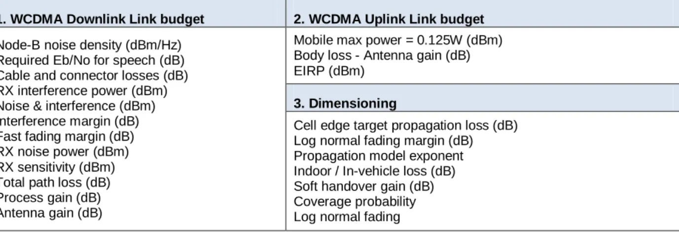
Link Budget for WCDMA1 The follow vendor specification parameter value should be known to estimate the system capacity and coverage.

Table 1: Vendor Specification Required for Calculating Link Budget 1. WCDMA Downlink Link budget 2. WCDMA Uplink Link budget

Node-B noise density (dBm/Hz) Required Eb/No for speech (dB) Cable and connector losses (dB) RX interference power (dBm) Noise & interference (dBm) Interference margin (dB) Fast fading margin (dB) RX noise power (dBm) RX sensitivity (dBm) Total path loss (dB) Process gain (dB) Antenna gain (dB)

Mobile max power = 0.125W (dBm) Body loss - Antenna gain (dB) EIRP (dBm)

3. Dimensioning

Cell edge target propagation loss (dB) Log normal fading margin (dB) Propagation model exponent Indoor / In-vehicle loss (dB) Soft handover gain (dB) Coverage probability Log normal fading

1: For simulation task this values are tailored

3.4 Monitoring and Optimisation

The wireless network and its devices need to be monitored continuously and there are several reasons for monitoring. The main objective is to monitor the network performance and system failure. The system log information is used for optimization.

Types of techniques used for optimization:

1. Monitoring the performance of the network using the “Network Management System (NMS)” 2. “Field test” is carried out in order to validate the network performance from the user’s point of view.

The NMS provides valuable information about the various parameters of the network and in this type of system it is possible to collect executive reports for maintenance purpose. However, the field testing is an extremely best approach to receiving coverage perspective information about cellular network in different geographical areas.

3.5 Key Performance Indicator (KPI)

KPI is based on a mathematical formula; it is used as a tool for determining network performance, optimizing the network, understand root causing problem in the network and to troubleshoot. Field measurements and KPI monitoring are required for optimization.

– Interference (Pilot pollution due to high-elevation sites with large RF coverage) – Call establishment success rate, (Call blocking) blocking rate, packet call delay – Handovers per cell (all types) Soft handover overhead (usually lower than 40 percent) – Delay and throughput of PS services (FTP, Web, Streaming, MMS, PoC)

– Overload situations (interference, lack of element capacity) – Average Transmitting and receiving power of UE

3.6 Performance Measurement Techniques

Energy per bit to noise ratio density (Eb/No): The receiver sensitivity level can be calculated using minimum RF

signal at the input point of receiver to supply the output (after data demodulation). For digital wireless system the quality of the receiver input-signal is expressed in term of (Eb/No) and the output-signal is expressed in terms of BLER (Block Error Rate) or BER (Bit Error Rate) [8].

- - - (1)

Where Rc the chip rate Rb is the user’s bit rate and C is the minimum required signal-power at the receiver input. Bit energy to interference ratio (Eb/I0): The required bit-energy to interference ratio (Eb/I0) is used to calculate the uplink capacity, the below equation (2) is used for approximately calculate

- - - (2)

Where Eb is the bit energy received, Io is the total Interference, S is the power of each UE received at the base station, PG is the Processing-Gain, F is the Noise-Figure, W is the transmission bandwidth, is the voice activity, Nth is the thermal noise power density, is the adjacent cell interference factor, is the overhead power factor, N is the number of users, NCM is the number of users in the compressed mode, and is the average increasing power from the compress mode users.

A new approach of combining the RSCP and pilot-to-interference ratio (Ec/Io): In the following journal [8], that proposed the (Ec/Io), is suitable for heavy traffic load and the “Received Signal Code Power of Common Pilot Channel” (RSCPCPICH) is applicable for low traffic load. Further, the method of combined pilot RSCP triggering and pilot Ec/Io concept was proposed to guarantee the border cell handover performance under various traffic loads. Ec/I0 = RSCPCPICH/RSS

Ec/I0 = RSCPCPICH/RSSI - - - (3)

133

In W-CDMA uplink, RRM approach is relation to interference power have been extensively investigated [5], [7]. In these schemes, the Node-B manages traffic to satisfy the constraint of

- - - (1)

where K is the number of active users, Iother is the interference from neighbour cell or other cells, I0,max is the maximum total interference, SF is the spreading factor, N0 is the noise power density and Eb is the bit energy. Normally, the allowable interference-to-noise-ratio

- - - (2)

In general the transmission rate varies for different types of application, so the nose-B is required to manage traffic to expectations [2].

4 System Implementation

4.1

Scenario Designing

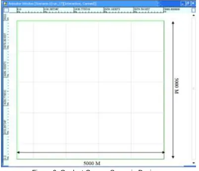
The canvas is used for design the scenario and its dimension is 5000M*5000 meter altitude, considered as real-time terrestrial. The component can be placed manual or automatically in a random manner using the random seed place command, but in this scenario the network component are placed manually.

Figure 9: Qualnet Canvas Scenario Designer

4.2

Steps in Designing and Configuring U

air Interface, Node-B and UE

Step 1: Defining channels for transmitter and receiver.

Table 2: Channel Parameters

Parameters Channel-1 (Uplink) Channel-2 (Downlink)

Channel Frequency 1.95 GHz 2.15 GHz

Propagation Model Statistical Statistical

Propagation Limit -152.0 dbm -152.0 dbm

Propagation Shadowing Model Constant Constant

Propagation Shadowing Mean 4.0dB 4.0dB

Reasoning for above choice value: W-CDMA FDD required two channels for Uplink and downlink. Signals with powers below propagation-limit- 152 dbm will not be delivered. The FDD, W-CDMA frequency range is 1920-1980 MHz paired uplink and 2110-2170 MHz paired downlink. The channel spacing is 5 MHz and the raster is 200 kHz. So to operate the network in W-CDMA FDD mode, it required 3 to 4 channels in general; channels can be assigned according to the network speed and capacity, as follows 12 channels (12 x5 MHz) or 4 channels (2x20 MHz). In this simulation centre frequency (carrier frequency) is used.

Step 2: Creating wireless interfaces for Node-B and UE

To create a wireless interface between the node-B and UE, wireless subnet has to be defined and parameter values are configured in the wireless subnet. The wireless subnet is similar to a hub and it is determined by the MAC-layer of the qualnet UMTS Library. In addition a wireless subnet is placed in the canvas and appropriate node-b and UE are connected to the subnet to form a wireless connection. Listenable channel masking is done for UE and Node-B; where all UE’s is allowed to listen for downlink channel and all Node-B listen to the uplink channel. So it set 1 to listen to the channel.

Table 3: Channel Settings

Parameter Value

Phy-listenable-channel-mask 11

Phy-listenable-channel-mask 11

Phy-temperature 290.0

Phy-noise-factor 10.0

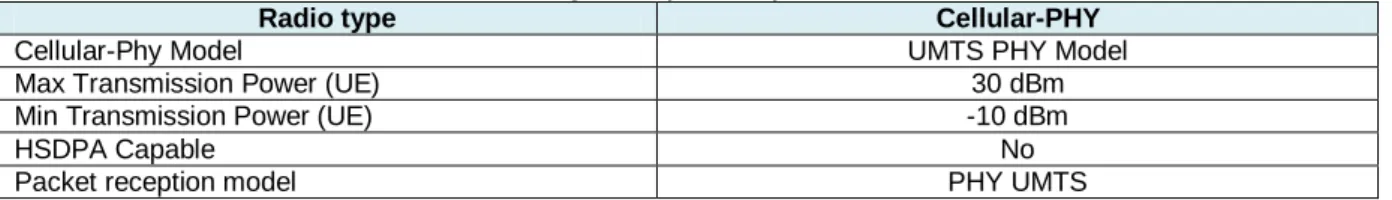
Step 3: Configuring MAC and physical layer properties

Table 4: Setting the Physical Layer Parameters

Radio type Cellular-PHY

Cellular-Phy Model UMTS PHY Model

Max Transmission Power (UE) 30 dBm

Min Transmission Power (UE) -10 dBm

HSDPA Capable No

Packet reception model PHY UMTS

The transmitting power are varied from -10dB to 30dB, depending on the traffic and data rate. Even if the Node-B send a command to increase the transmitting power but it is bounded around 30db. Physical and MAC layer properties are configured in the Step 2 of wireless subnet link as well.

Step 4: Defining UE’s and configuring

Table 5: Configuring UE Layer 3 Parameters

Parameter Value

Min Cell Selection Rx Level -95 dBm

Cell Search Threshold -80 dBm

Cell Reselection Hysteresis 3.0 dB

Step 5: Configuring the Node-B

Table 6: Configuring Node-B Layer-3 Parameters

Parameter Value

Downlink Channel 0

Uplink Channel 1

Min Cell Selection Rx Level -95 dBm

Cell Search Threshold -80 dbm

Cell Reselection Hysteresis 3.0 dB

The “Min cell selection Rx level” is used for initial cell selection, when UE is powering on. When a cell searching is initiated by UE, it receives different threshold voltage from different cell; now the UE will rank the received signals from different cell and select the strongest signal. These kinds of threshold triggering applicable for both intra frequency and inter frequency cell searching. The reselecting hysteresis value is used for reselecting the cell; if the hysteresis value is below 3db then it is allowed UE to reselecting the cell. In UMTS, selecting and reselecting process is based on algorithm. In general, increasing the hysteresis value, gives a high priority to the serving cell and decreasing this hysteresis value makes the cell reselection more often for a quality cell.

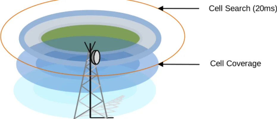
Step 6: Configuring the antenna setting (Change for different Scenario)

In this scenario three Node-B’s are deployed in the design with different parameter setting to cover the terrain altitude. To form different cell topologies the Node-B transmitting power (downlink) and height of the antenna are varied because these parameters are directly related to the cell coverage. The control channel broadcasting cell related information periodically in its location and its value is 20ms.

135

Figure 10: Cell Range Defining Parameter

4.3

Designing and Configuring the Core Network

The core network consists of RNC, SGSN, HLR and GGSN, the connection between all this are point to point link.

Step 1: Configuring the RNC, enabling point to point connection with Node-B, SGSN, RNC and Soft Handover. The RNC is connected to the Node-B and SGSN, the connection between all these nodes are based on point to point link.

Table 7: Configuring Threshold Power for RNC

Parameter Value

Soft HO AS Threshold 3.0 dB

Soft HO AS Threshold Hysteresis 1.0 dB

Soft HO AS Replace Hysteresis 1.0 dB

Figure 11: Soft Handover Region

Defining and Soft Handover Threshold in RNC: The “Soft HO AS Threshold” is used to micro diversity, if the current active threshold is below 3db then RNC is allowed to add a new cell or take off the connection of UE from active set cell. If the power of “Soft HO AS Threshold Hysteresis” is below 1db then it will enable the soft handover and to replace the cell “Soft HO AS Replace Hysteresis” is applied. The connection between the 1, Node-B-2 and Node-3 are connected to the RNC using the single hop point to point connection.

Step 2: Configuring the SGSN, enabling point to point connection with RNC, GGSN and HLR.

The Node ID of HLR and GGSN is configured in SGSN as addresses to routing the packets. The connection between SGSN and other can support multiple hop point to point connection.

RNC

Cell Coverage Cell Search (20ms)

“Soft handover Region” Threshold value configure,

Step 3: Configuring the HLR with SGSN and enabling point to point access.

Step 4: Configuring the GGSN.

It is an assumption that the entire network maintains only one HLR. The call tracing and the packet use the network or node ID. So no additional features are required to configure the HLR.

5 Computational Experiment and Results

5.1

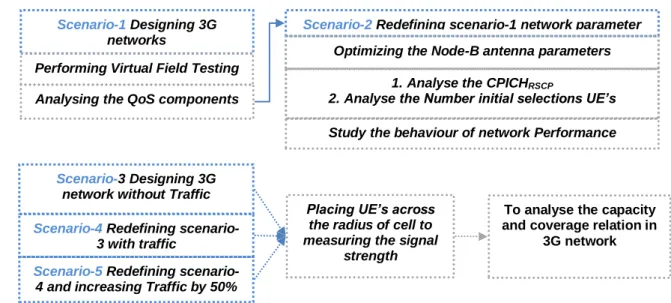
Overview of Experiments

Figure 12: Overview of Simulation Scenarios

5.2

Perform Virtual Field Test

The scope of this scenario is to design a 3G network and to perform virtual field testing.

For this scenario, the test approach is first by identifying the major test components, which a have relation with QoS. The test design however, beside the case study, it is identified the following component need to measured:

 Measuring UE primary CPICH Ec/No

 Measuring UE's Primary Node-B CPICHRSCP

 Measuring the number of cell search performed by UE’s.  Measuring the number of cell reselection performed by UE’s  Measuring the number of UE’s cell initial selections with the network  Comparing the number of UE’s attach request and attach accept messages  Comparing the number of UE’s service request and service accept messages

Next the test execution, where the test are executed using the qualnet analyser and visualizer as follows:  The measurement 1 and 2 are executed using the “Dynamic Statistics Metric”

 The measurement from 3 and 6 are executed using the “Analyser”

5.3

Network Scenario Implementation Procedure

According to the implementation procedure followed in chapter-4; the air Interface configuration, core network configuration and RNC configuration remain same, but the node component, traffic and the antenna setting changes as below:

Parameter Address

My Home Location Register Server 1

Scenario-3 Designing 3G network without Traffic

Placing UE’s across the radius of cell to measuring the signal

strength

To analyse the capacity and coverage relation in

3G network Scenario-4 Redefining

scenario-3 with traffic

Scenario-5 Redefining scenario-4 and increasing Traffic by 50%

Scenario-1 Designing 3G networks

Performing Virtual Field Testing

Study the behaviour of network Performance Analysing the QoS components

Scenario-2 Redefining scenario-1 network parameter Optimizing the Node-B antenna parameters

1. Analyse the CPICHRSCP

137

Table 8: Total Number of Node in the Scenario-1

Parameter Node-ID Total Number of Nodes

HOSTNAME UMTS-HLR1 [1] 1

HOSTNAME UMTS-SGSN2 [2] 1

HOSTNAME UMTS-GGSN3 [3] 1

HOSTNAME UMTS-RNC4 [4] 1

HOSTNAME UMTS-Node-B [5] to [7] 3

HOSTNAME (CBR Traffic Nodes) [8] to [13] 6

HOSTNAME UMTS-UE [14] to [55] 42

Table 9: Node-B Antenna Parameters

Parameter Node-B ID-5 Node-B ID-6 Node-B ID-7

Antenna Model Omni directional Omni directional Omni directional

TX-power Max 33 dB 33 dB 35 dB

Antenna Height 2.5 m 2.5 m 3.5 m

Antenna Efficiency 0.51 0.51 1.07

Antenna Mismatch Loss 0.31 dB 0.31 dB 0.31 dB

Antenna Cable Loss 0.21 dB 0.21 dB 1.4 dB

Antenna Connection Loss 0.21 dB 0.21 dB 0.21 dB

Antenna Gain 0.0d dB 0.0 dB 0.0 dB

5.3.1 Results and Analysis

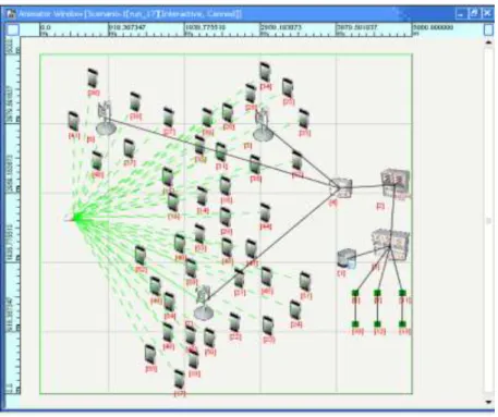
Topology View of Designed Network: The below figure shows the logical connection between the network elements.

Figure 13: Topological View of Designed Network

The cloud shown in the canvas is wireless subnets, which acquires the WCDMA wireless properties and provide connectivity between the Node-B and UE’s. The channel configuration and its setting are is same as explained in the chapter-5. The Constant Bit Rate (CBR) Traffic is used to generate the background traffic with particular UE’s.

Traffic Flow of Designed Network

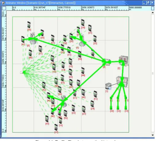
Figure 14: Traffic Flow between the Networks

The total active background traffic in each node is with UE’s are 4. The picture-21 we can view,

 The CBR traffic is established with UE’s (26 and 28) and the connection with UE’s (35 and 25) is not established.

 The CBR traffic is established with UE’s (39 and 41) and the connection with UE’s (27 and 37) is not established.

 The CBR traffic is established with UE’s (42, 48, and 49) and the connection with UE’s (21) is not established.

Radiation Pattern of Node-B’s

139

5.3.2 Virtual Field Test and Analysis

1. Measuring UE Primary CPICH Ec/No

Energy per chip to noise ratio density is measured for different time interval using the real time interface using qualnet - visualizer “Dynamic Statistics Metric”. The average of Ec/No is calculated to estimate the quality of the received signal.

Figure 17: Measuring Ec/No for Time Interval-5 2. Measuring UE's Primary Node-B CPICHRSCP

CPICHRSCP is measured for only single time interval because all UE’s are not in motion.

Figure 18: CPICHRSCP Measurement

5.3.3 Comparing and Analyse of Ec/No and CPICH

Measurement

Figure 19: Comparing Ec/No and CPICHRSCP Measurement

In the above graph the Ec/No and CPICHRSCP are compared; in general Ec/No should be sufficiently high to recover the user information. Here it is observed that the Ec/No value of some UE’s are very low, which is not sufficient for UE’s to make the connection with Node-B. It is also observed that the Ec/No value rise when CPICHRSCP is sufficient, further coverage is also directly related with data rate. The graph concludes that there is need for optimization.

CPICHRSCP Ec/No CPICHRSCP Range -97dbm to -79.5dbm CPICHRSCP Range -79.5dbm to -62dbm

141

Figure 20: Comparison Graph of UE Command Messages

0

2

4

6

8

10

12

14

UE-14

UE-15

UE-16

UE-17

UE-18

UE-19

UE-20

UE-21

UE-22

UE-23

UE-24

UE-25

UE-26

UE-27

UE-28

UE-29

UE-30

UE-31

UE-32

UE-33

UE-34

UE-35

UE-36

UE-37

UE-38

UE-39

UE-40

UE-41

UE-42

UE-43

UE-44

UE-45

UE-46

UE-47

UE-48

UE-49

UE-50

UE-51

UE-52

UE-53

UE-54

UE-55

No of cell reselection

No of initial cell selection

No of cell search performed

7. Comparing the Number of UE’s Service Request and Service Accept Messages

Figure 21: UE's Number of Service Request Message Sent and Service Accept Message Received

5.3.4 Network Quality Assessment

Based the first four virtual measurements, it is identified that there is coverage gap in between the cells; therefore cover of the network has to be optimised. Also by the observing and measuring the KPI parameter through the UE’s Logs, it is identified that the capacity is sufficient because in the measurement-6 there is no attach reject messages. In the measurement-5 it is observed that, out of 42 UE’s only 22 UE’s are connected with the network. So the cells covered 52.4 percent of UE’s, according KPI its worst coverage ratio and need to be optimized.

The Scope of the Scenario-2 is to optimize the scenario-1 design of 3G network for better coverage.

Procedure of optimization: To identifying cell coverage gaps and number of UE’s out of coverage. The following Parameters changed for optimum coverage.

Table 10: Parameters Changed for Optimum Coverage

Parameter Node-B ID-5 Node-B ID-6 Node-B ID-7

Antenna Model Omni directional Omni directional Omni directional

TX-power Max 32 dB 29 dB 35 dB

Antenna Height 5.3 m 5.3 m 8.54 m

5.3.5 Result and Analyse

1. Optimized Network CPICHRSCP Measurement

Figure 22: Optimized Network CPICHRSCP Measurement

0

2

4

6

UE

-14

UE

-16

UE

-18

UE

-20

UE

-22

UE

-24

UE

-26

UE

-28

UE

-30

UE

-32

UE

-34

UE

-36

UE

-38

UE

-40

UE

-42

UE

-44

UE

-46

UE

-48

UE

-50

UE

-52

UE

-54

143

2. Comparing Scenario-1 and Scenario-2 UE’s Cell Initial Selections

Figure 23: Comparing Scenario-1 and Scenario-2 UE’s Cell Initial Selections

In above graph, it clearly shows that the coverage of the cell is optimized for the best without implementing additional Node-B. The power and the antenna height are adjusted to maximise the coverage range.

5.4

Scenario-3, 4 and 5: To Analyse Capacity and Coverage Interlink

To investigating the relation between the capacity and coverage under various traffic conditions. The channels for transmitter and receiver, wireless interfaces for Node-B and UE, MAC layer and physical layer all these properties and it is configuration remain the same as implemented as mentioned earlier. The number network entity various as follow:

0

2

4

6

8

UE-14

UE-16

UE-18

UE-20

UE-22

UE-24

UE-26

UE-28

UE-30

UE-32

UE-34

UE-36

UE-38

UE-40

UE-42

UE-44

UE-46

UE-48

UE-50

UE-52

UE-54

A

xi

s

Ti

tl

e

Scenario-2 No of UE's Cell Initial

Selections

Scenario-1 No of UE's Cell Initial

Selections

Table 11: Total Number of Node in the Scenario-2, 3 and 5

Parameter Node-ID Total Number of Nodes

HOSTNAME UMTS-HLR1 [1] 1

HOSTNAME UMTS-SGSN2 [2] 1

HOSTNAME UMTS-GGSN3 [3] 1

HOSTNAME UMTS-RNC4 [4] 1

HOSTNAME UMTS-Node-B [5] 1

HOSTNAME (CBR Traffic Nodes) [6] to [13] 8

HOSTNAME UMTS-UE Scenario-3, 4 [14] to [55] 42

Scenario-5 [14] to [84] 64

Table 12: Node-B Antenna Parameters

Parameter Node-B ID-5

Antenna Model Omni directional

TX-power Max 29db

Antenna Height 7.1M

Antenna Efficiency 0.80

Antenna Mismatch Loss 0.31db

Antenna Cable Loss 0.21 db

Antenna Connection Loss 0.21 db

Antenna Gain 0.0db

5.4.1 Test and Measurement Strategy

To measure the range of cell coverage with and without traffic, an ideal mode UE’s are used for measuring the CPICHRSCP. These UE’s are dimensioned equally from the radius of the cell.

Figure 24: Coverage Test Strategy

Figure 25: A Typical Topology View of Scenario-3 and Scenario-4

14 ideal UE’s (UE-14 to UE-27) are equally positioned in both x axis and y axis at the distance of 150m from the radius of Node-B.

145 Measuring the CPICHRSCP

Table 13: Scenario-3 CPICHRSCP Measurement UE’s UE-14 and

UE-21 UE-15 and UE-22 UE-16 and UE-23 UE-17 and UE-24 UE-18 and UE-25 UE-19 and UE-26 UE-20 and UE-27 Radius 150m 300m 450m 600m 750m 900m 1050m CPICHRSCP (dbm) -63 -70 -73 -75.6 77.2 78.8 80.8 -63 -70 -73 -75.6 77.2 78.8 80.8 Average (dbm) -63 -70 -73 -75.6 77.2 78.8 80.8 Scenario-4

The scenario-3 is redesigned by including the CBR traffic flow with UE’s. From the UE-22 to UE-44 is connected to the CBR traffic, all UE’s traffic begin and ends at the same time. This is to analyse coverage and capacity issues. The traffic file is attached in the appendix.

Table 14: Scenario-4 CPICHRSCP Measurement

UE’s UE-14 and

UE-21 UE-15 and UE-22 UE-16 and UE-23 UE-17 and UE-24 UE-18 and UE-25 UE-19 and UE-26 UE-20 and UE-27 Radius 150m 300m 450m 600m 750m 900m 1050m CPICHRSCP (dbm) Trail-1 -67.7 -74.3 -78 -80.4 -82 -84 -85.2 Trail-2 -66 -71.1 -76 -78 -80 -81 -83 Trail-3 -67.5 -73.8 -77 -79.7 -82 -83.5 -85.3 CPICHRSCP Average (dbm) -67 -73 -77 -79 -81.6 -82.8 -84.6 Scenario-5

The scenario-4 is redesigned by increasing the CBR traffic flow between UE’s to 75 percent. From the 22 to UE-64 is connected to the CBR traffic, all UE’s traffic begin and ends at the same time.

Figure 26: Topology View of Scenario-5

Table 15: Scenario-4 CPICHRSCP Measurement

UE’s UE-14 and

UE-21 UE-15 and UE-22 UE-16 and UE-23 UE-17 and UE-24 UE-18 and UE-25 UE-19 and UE-26 UE-20 and UE-27 Radius 150m 300m 450m 600m 750m 900m 1050m CPICHRSCP (dbm) Trail-1 -69 -75 -78.2 -80 -82.8 -83.9 -86 Trail-2 -68 -74.7 -77.7 -80 -82.5 -84 -85.5 Trail-3 -68.7 -75 -78 -80 -82.8 -83.7 -86 CPICHRSCP Average (dbm) -68.6 -74.9 -77.9 -80 -82.7 -83.9 -85.8

5.4.2 Comparing the CPICH

Value of Scenario-3, 4 and 5

Table 16: CPICHRSCP Comparison Graph

CPICHRSCP Average (dbm) 150m 300m 450m 600m 750m 900m 1050m

Scenario-1 -63 -70 -73 -75.6 -77.2 -78.8 -80.8

Scenario-2 -67 -73 -77 -79 -81.6 -82.8 -84.6

Scenario-3 -68.6 -74.9 -77.9 -80 -82.7 -83.9 -85.8

Figure 27: CPICHRSCP Comparison Graph

Figure 28: Radar Graph for CPICHRSCP Comparison

From the comparison graphs it is observed that scenario-3 has large cell radius compared to the other scenarios and also the CPICHRSCP value of scenario-3 varies from 2.5dbm to 3dbm for 150m distance. However, in the scenario-4 the traffic is introduced for UE-28 to UE-44 seemingly the cell traffic is high because the UE’s are configured to burst at the same period of time, at the same instant of time the CPICHRSCP values are measured for different time interval and its average value difference is from 2dbm to 3dbm comparing with scenario-3. Similarly for scenario-5 the CPICHRSCP value decreases when the number of CBR traffic is increased to 75 percent. From this computational experiment it is clearly observed when traffic is enormous then cell breathing occurs.

-88

-86

-84

-82

-80

-78

-76

-74

-72

-70

-68

-66

-64

-62

-60

-58

-56

-54

-52

-50

Scenario-3 CPICHRSCP

Average

-90

-85

-80

-75

-70

-65

-60

-55

Radius 150

Radius 300

Radius 450

Radius 600

Radius 750

Radius 900

Radius 1050

Scenario-3 CPICHRSCP Average

Scenario-4 CPICHRSCP Average

Scenario-5 CPICHRSCP Average

147

6 Conclusion

6.1

Statement of the Result

In this project different types of scenario are designed and tested to analyse the behaviour of network subsystems. However, it clearly understood the coverage and capacity has to be planned together for 3G Networks unlike GSM because all users share the same air interface resource, consequently they cannot be dimensioned and analysed separately. From the Scenario-1 the QoS of network is attained by field testing and the beneficial of field testing measurements are used for further optimizing of the network QoS. In the Scenario-3, 4 and 5 are designed to analyse the interlink between coverage and capacity from the computational experiment a major problem is observed as follows,

6.1.1 Observed Problem

In the Scenario-5 it is clearly observed that complicated interference is influenced by both capacity and coverage planning in the following aspects. Cell breathing is occurred when the traffic exceeds and multiple near-far UE spread over the cell. The link budget is combination with interference margin, which raise the noise level produced by greater cell load. Consequently by raising the cell load, the cell coverage shrinks.

Figure 29: Capacity and Coverage Interlink

6.2

Recommended Further Work

To analyse and predict the behaviour of 3G network in real-time, the emulation approach is well suited “Emulating UTRAN to perform virtual testing”.

Figure 30: Mapping UTRAN with Emulation Approach

The emulation concept is to replace the real-time system, when we emulate the network components it perform the same as a real-time physical system, perhaps speed. In the emulation concept UE, UTRAN and core Network are an individual PC’s station mapped according to their architecture. Qualnet software has the emulation library and UTMS library, which can be used to implement this kind of approach.

Uu

UTRAN Core Network

l

UE Emulator

UTRAN Emulator

CN Emulator Cell coverage shrinking, due

increased traffic

(High Data Rate) Traffic Increase

Actual cell coverage Cell Radius

References

[1] 3GPP Workshop News on “Evolution of the 3G Mobile System started with the RAN Evolution Work Shop”, November 2-3, 2004, Toronto, Canada.

[2] E. Babich, L. Deotto, and E. Vatta. Transmission of embedded VBR multimode encoded speech on UMTS common packet channels, IEEE VTS-Fall VTC 2000, 52nd Vehicular Technology Conference, 2000, vol. 3, pp. 1405-1411.

[3] E. Fledderus, and L. Jorguseski. Radio resource allocation in third generation mobile communication systems, IEEE Communications, vol. 39, no. 2, pp. 117-123, 2001.

[4] M. C. Jeruchim, K. S. Shanmugam, and P. Balaban. Simulation of Communication Systems. New York: Kluwer Academic/Plenum Publication, New York, 1992.

[5] J. Perez-Romero, O. Sallent, N. Garcia, and R. Agusti. On managing uplink videophone and web browsing traffic in UTRA W-CDMA, 14th IEEE Proceedings on Personal, Indoor and Mobile Radio Communications, PIMRC, 2003, vol. 2, pp. 1166-1170.

[6] Roy Blake, Wireless Communication Technology, 2nd., Publisher Delmar Thomson Learning, pp. 04.

[7] O. Salient, J. Perez-Romero, and R. Agusti. Optimizing statistical uplink admission control for W-CDMA, IEEE 58th Vehicular Technology Conference, VTC 2003-Fall, 2003, vol. 2, pp. 811-815.

[8] J. Viterbi, and A. M. Viterbi. Earlang capacity of a power controlled CDMA system, IEEE Selected Areas in Communcations, vol. 11, no. 6, pp. 892-900, 1993.