ERROR BOUNDS FOR SURFACE AREA ESTIMATORS BASED ON CROFTON’S FORMULA

ERROR BOUNDS FOR SURFACE AREA ESTIMATORS BASED

ON CROFTON’S FORMULA

M

K

D

M

1_{Department of Mathematical Sciences, University of Aarhus, 8000 Aarhus, Denmark;}2_{Insitute of Stochastics,}

Ulm University, 89069 Ulm, Germany

e-mail: [email protected], [email protected]

(Accepted September 1, 2009)

ABSTRACT

According to Crofton’s formula, the surface area S(A) of a sufficiently regular compact set A in Rd _is proportional to the mean of all total projections pA(u) on a linear hyperplane with normal u, uniformly averaged over all unit vectors u. In applications, pA(u)is only measured in k directions and the mean is approximated by a finite weighted sumSb(A)of the total projections in these directions. The choice of the weights depends on the selected quadrature rule. We define an associated zonotope Z (depending only on the projection directions and thequadrature rule), and show that the relative errorSb(A)/S(A)is bounded from below by the inradius of Z and from above by the circumradius of Z. Applying a strengthened isoperimetric inequality due to Bonnesen, we show that the rectangular quadrature rule does not give the best possible error bounds for d=2. In addition, we derive asymptotic behavior of the error (with increasing k) in the planar case. The paper concludes with applications to surface area estimation in design-based digital stereology where we show that the weights due to Bonnesen’s inequality are better than the usual weights based on the rectangular rule and almost optimal in the sense that the relative error of the surface area estimator is very close to the minimal error.

Keywords: associated zonotope, Crofton formula, digitization, isoperimetric inequality, minimal annulus, perimeter, surface area.

INTRODUCTION

One common approach to approximate the surface area S(A) of an unknown set A _⊂ Rd _{from its}

digitization is based on a discretization of Crofton’s formula. We discuss the worst case error introduced by the discretization of the rotational integral in dependence of the quadrature rule chosen. As the methods apply generally to surface area estimators based on Crofton’s formula, we describe them in a general framework and return to its application to digital images in the third section, entitled “Error Bounds for Digital Surface Area Estimators”.

Throughout the paper a direction is a vector on the unit sphere Sd−1 _in Rd_{. If u is a direction, u}⊥

denotesthe linear hyperplane with normal u, and er,u

isthe straight line with direction u through r_∈u⊥. Let

A_⊂Rd _{be afull-dimensionalcompact set in the class} U_{PR; (definitions can be found in the next section). A} special case of Crofton’s formula (Rother and Z¨ahle, 1990) expresses the surface area S(A)of A in terms of the Euler characteristicχof linear sections

S(A) = 2 γd

Z

Sd−1

Z

u⊥χ(A∩er,u)drµ(du). (1)

Hereγd= (2κd−1)/(dκd), whereκd is the volume of

the d-dimensional unit ball, and µ is the normalized

Haar measure on the unit sphere Sd−1_{; see, e.g.,} Schneider and Weil (1992, p. 18), but note the different normalization.For sets A that are not full-dimensional, Eq. 1 still holds if its left hand side S(A) is defined in such a way that lower dimensional parts of A are counted twice.The inner integral ofEq.1,

pu=

Z

u⊥χ

(A_∩er,u)dr, (2)

is called total projection of A in direction u, as it is obtained by measuring the (d₋1)-volume of the orthogonal projection of A on u⊥ with multiplicities.

In Eq. 2 the integration is understood with respect to the Lebesgue measure on u⊥. If total projections can be determined exactly for finitely many directions

u1, . . . ,uk∈Sd−1, say, a k-point quadrature rule can be

used to discretize the outer integral in Eq. 1 and one obtains the approximation

b

Sd_k(A) = 2

γd k

∑

cipu_i, (3)

which depends on the choice of weights c1, . . . ,ck≥0.

To assure that the quadrature rule is exact whenever

A is a ball, we assume throughout that the weights

spherical Voronoi cells generated by _{u1, . . . ,uk} on S1_{. This geometric interpretation generalizes readily}

to higher dimensions. If _{P1, . . . ,Pk} is the spherical

Voronoi tessellation of Sd−1 _{generated by the set of}

projection directions_{u1, . . . ,uk}withui∈Pithen the

weights

cV_i =µ(Pi), i=1, . . . ,k,

will be called Voronoi weights associated to

{u1, . . . ,uk}. These weights are commonly used in applications for d =2,3. In the special case where

d=2 and u1, . . . ,ukare equidistant, the weights for the

rectangular quadrature rule (Voronoi weights) coincide with those for the trapezoidal quadrature rule.

The discretization of the spherical integral introduces a bias, which typically depends on the set A. We are interested in the worst case behavior. Already Steinhaus (1930) treated the special case where d=2,

k is even, and{u1, . . . ,uk} forms an equidistant set of points in S1_{. ForS}b2

k(A), given by Eq. 3 with Voronoi

weights cV₁, . . . ,cV_k, he derived sharp bounds for the relative error:

π k

cos(π/k)

sin(π/k) ≤ b

S2_k(A) S(A) ≤

π k

1

sin(π/k) . (4)

The left hand side and the right hand side of Eq. 4 are the endpoints of the interval of all possible relative errors, as A varies. Such an interval can be established without the assumption of equidistant directions and in all dimensions. We refer to this interval as error

interval in the following.

Using a translative Crofton formula in Section

“Error Bounds for Sbd_k(A)”, we will define an origin-symmetric convex body Z _⊂ Rd _{associated to the}

discretization, only depending on the projection directions and the quadrature rule. We will show in Lemma 1 that the relative error Sb_kd(A)/S(A) is in a sharp way bounded from below by (a multiple of) the inradius of Z and from above by (a multiple of) the outer radius of Z. Thus, the thickness of the minimal annulus of Z is proportional to the length of the error interval and describes the quality of the estimator. Given k projection directions, the quadrature rule (in other words, the values of the associated weights) that minimizes the minimal thickness of Z can typically only be determined numerically. In the planar case, we suggest to bound the thickness of the minimal annulus of Z from above by an isoperimetric deficit using a strengthened isoperimetric inequality due to Bonnesen. This isoperimetric deficit can be minimized with respect to all quadrature rules in closed form. The weights minimizing the isoperimetric deficit will be

called Bonnesen weights and are proportional to the lengths of the edges of a polygon circumscribing the unit disk and touching it exactly at the pointsu1, . . . ,uk. We will show that Voronoi weights are not minimizing the length of the error interval by giving an example where the Bonnesen weights yield better error bounds. We will determine the asymptotic behavior (as k_→ ∞) of the relative error for the Bonnesen weights in Theorem 4. At the end of the second section we will consider the case where the directionsu1, . . . ,uk ∈S1 are obtained using systematic random sampling onS1_. We will show that the coefficient of error of Sb_k2(A)

can be bounded from above by a geometric quantity involving Z, namely a multiple of the L2-distance between Z and its Steiner ball.

Inthe subsequent section we discuss error bounds for digital surface area estimators. The digitization of

A on a randomly translated, rectangular grid will be

considered. Asymptotic bounds for the expected value of the estimator for S(A)in the grid will be established. ”Asymptotic” relates here to increasing resolution of the grid. The vectors u1, . . . ,uk are chosen as grid directions, i.e.,normalized vectors connecting two grid points. These two grid points are usually neighbours and we will consider the4-, 8- and 16-neighborhood in 2D and the 6- and 26-neighborhood in 3D. For all these settings the Voronoi and Bonnesen weights together with the corresponding in- and circumradii r and R, respectively, will be computed analytically, except for the 26 directions in 3D where numerical methods will be used. We will compare the relative errors with the minimal error achieved by numerically optimizing the weights and show that the Bonnesen weights lead, at least in 2D, to smaller errors than the widely used Voronoi weights. We then restrict to quadratic grids in the plane and consider boundary length estimators based on pairs of grid points that are contained in some (n₋1)_×(n₋1) square of grid cells, n_≥2. This generalizes the case n=2, which corresponds to the boundary length estimator based on 8-neighbours. Theorem 7 considers such estimators for general n_≥2 and shows that the asymptotic mean relative error of b

Sd_k(A)for Bonnesen weights decreases as n−2.

The application of Bonnesen’s improved isoperimetric inequality restricts many of the above arguments to the two-dimensional case. In the last section we discuss the possibility of extensions to higher dimensions.

ERROR BOUNDS FOR

S

b

(

A

)

A set A _⊂Rd _{is full-dimensional, if its tangent}

to (d₋1)-dimensional Hausdorff measure. If A is topologically regular (A is the closure of its interior) and convex, it is also full-dimensional. The set A has positive reach if there isanε>0 such that each point in theε-neighborhood of A has a unique closest point in A.

Throughout the following we assume that A is an element of the familyU_{PRof all sets in}Rd _{which can}

be written as a finite union of compact sets A1, . . . ,Am

with positive reach such that any intersection Ti_∈IAi

with I_{⊂ {}1, . . . ,m_}is either empty or a set of positive reach, as well. In particular, convex bodies (nonempty compact convex subsets of Rd_{) and polyconvex sets}

(finite unions of convex bodies) are elements of U_PR. For A _∈ U_{PR the surface area measure S(A,·) of} order d₋1 is defined, and Eq. 1 holds with S(A) = S(A,Sd−1_{). If A is in addition full-dimensional, S(A)} coincides with the usual surface area of A.In view of the applications in digital stereology, it is convenient to extend the total projection mapping v_7→pvtoRd_\{o}

by positive homogeneity of degree 0. The translative Crofton formula

pv= 1

2_kv_k

Z

Sd−1|hu,vi|S(A,du) (5)

holds for almost all v_∈Rd_{; see Rataj (2002, Theorem} 2.1 and Theorem 2.3), where_hu,v_i is the usual inner product of u and v. If A is polyconvex,Eq.5 holds for

all v_∈Rd_{\ {o}.}

If v1, . . . ,vk ∈Rd\ {o} are such that Eq. 5 holds

with v=vi for all i=1, . . . ,k, then the definition of

b

Sd_k(A)in combination withEq.5 yields

b

Sd_k(A) = 1

γd

Z

Sd−1h(u)S(A,du), (6)

with

h := k

∑

ci

kvik|h

vi,_·i|. (7)

The key observation is that the integrand h is the support function of a convex body. We refer the reader to Schneider (1993) for relevant notions and concepts in convex geometry and only recall the most important facts here. The support function hK of a convex body K is given by

hK(u) =max{hx,ui: x∈K}, u∈Sd−1.

Here and in the following, we consider the support function as a function on the unit sphere. For convex bodies K and M and scalarsα,β_≥0, we have

αhK+βhM=h_αK⊕βM, (8)

where the Minkowski addition _⊕ of sets and the multiplication of a set with a scalar are understood pointwise. We will repeatedly use the monotonicity property,

K_⊂M _⇐⇒ hK≤hM, (9)

and the fact that the support function h_Bd of the

Euclidean unit ball Bd in Rd _{is the constant 1. Eq. 9}

implies in particular that any convex body is uniquely determined by its support function. Consequently, the definition,

δ2

2(K,M):= Z

Sd−1(hK(u)−hM(u))

2 du,

for convex bodies K and M, gives rise to the so-called

L2-metric δ2(·,·) on the family of convex bodies. The support function of the line segment[₋x,x]with endpoints ₋x and x_∈ Rd _{is |hx,·i|. Due to Eq. 8,}

the function h in Eq. 7 is the support function of a finite sum Z of line segments. Such sets are called

zonotopes and play a prominent role in functional

analysis, convex and stochastic geometry (see, e.g., Goodey and Weil, 1993 and the references therein). Explicitly, we have

Z=c1[−u1,u1]⊕. . .⊕ck[−uk,uk], (10)

with the unit vectors ui = vi/kvik for i =1, . . . ,k.

In view of Eq. 6 the approximation Sbd_k(A) can be expressed in terms of the associated zonotope Z, as

b

Sd_k(A) = 1

γd

Z

Sd−1hZ(u)S(A,du). (11)

To obtain lower and upper bounds ofSb_kd(A), we have to find maxima and minima of hZ. Due to Eq. 9, r _≥0 is the minimum of hZ on Sd−1 if and only

if rBd is the largest ball contained in Z. Similarly,

R_≥0 is the maximum of hZ, if and only if RBd is the

smallest ball containing Z. With these optimal values of 0_≤r_≤R, the set RBd_\rBd is called the minimal

annulus of Z. The difference R₋r is called the width of the minimal annulus and denoted by T(Z). For later reference we summarize this geometric interpretation for polyconvex sets (for whichEq.5 holds for arbitrary

v₆=o). As formulations forU_{PR-sets are obtained in a} straightforward manner, we will restrict to polyconvex sets from now on.

Lemma 1 Let A _⊂ Rd _{be a polyconvex set with} positive surface area, and fix k_≥2 and v1, . . . ,vk _∈ Rd_{\ {o}. Let}γ_{d = (2}κ_d−1)/(dκ_{d). IfS}bd

k(A) is given byEq.3, then the sharp bounds

r γd ≤

b S_kd(A)

S(A) ≤ R

γd , (12)

Proof As R is the maximum of hZ on Sd−1, it

follows from Eq. 11, that

b

Sd_k(A)_≤ R γdS(A) ,

which yields the upper bound. The lower bound follows analoguously from Eq. 11 and the fact that r is the minimum of hZ onSd−1.

That the bounds in the above Lemma are sharp follows from the next example.

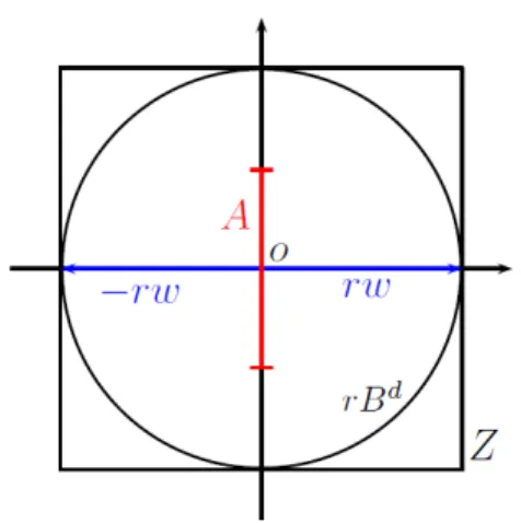
Example 2 Fix k_≥2, u1, . . . ,uk _∈Sd−1 _{and weights}

c1, . . . ,ck ≥ 0 for a quadrature rule. Define Z according to Eq. 10. Due to symmetry, the ball rBd touches the boundary of Z in at least two antipodal points rw and ₋rw, w _∈ Sd−1_{. Let A be a ball of}

(d₋1)-volume 1/2 in the hyperplane w⊥. (As A is lower dimensional, the proper interpretation of S(A) is twice the (d₋1)-dimensional Hausdorff measure, so S(A) = 1.) The surface area measure of A is

concentrated on the points w and₋w, and hZcoincides in both of these directions with r, soEq.11 implies

b

S_kd(A) = 1

γd

Z

Sd−1rS(A,du) =

r γd

S(A),

and equality holds on the left hand side ofEq.12.

Fig. 1 illustrates this for d=2, k=2, u1= (1,0)⊤,

u2 = (0,1)⊤ and c1 =c2 =1/2. Obviously A is not

topologically regular, but it can be approximated by a sequence of topologically regular convex bodies (Am) in such a way that limm→∞Sbdk(Am)/S(Am) =

b

S_kd(A)/S(A). This implies that the left hand side of Eq. 12 cannot be improved, even if we restrict considerations to topologically regular sets. To show that the second inequality inEq.12 is sharp, a similar argument can be used, if _±w are directions for which hZ becomes maximal, and thus coincides with R.

Fig. 1.A possible set A for the case where Z is the unit cube; see Example 2.

THE TWO-DIMENSIONAL CASE

In the following, we will restrict to the case d =

2, although some of the concepts can be transferred to higher dimensions. As the aim is to minimize the length of the error interval of Sb2_k(A) in Eq. 6, the difference R₋r should be as small as possible.

This can be achieved by an appropriate choice of the weights c1, . . . ,ck. To obtain an exact value for the

integral inEq.6 in the case where A is a disk, we must assume that the weights sum up to one.It follows from Schneider (1993), that c1+. . .+ck =1 is equivalent to the condition that the zonotope Z given byEq. 10 has perimeter 4. LetZ _{be the family of all zonotopes} that can be written as sum of line-segments parallel to given unit vectors u1, . . . ,uk. LetZ4 be the family of those Z_∈Z _{that have perimeter 4. We are therefore} faced with the problem of finding a zonotope Z∗_∈Z₄ that satisfies

T(Z∗) =min_{T(Z): Z_∈Z_{4}. (13)}

If

Z∗=c∗₁[₋u1,u1]⊕. . .⊕c∗k[−uk,uk],

then c∗₁, . . . ,c∗_k≥0 are the best weights inEq. 3, in the sense that among all weights summing up to one they yield the shortest interval of possible relative errors. A solution Z∗ of the optimization problem in Eq.13 always exists due to a compactness argument based on the Blaschke selection theorem.

For asymptotic results, it is enough to replace the objective function in Eq. 13 by a simpler one. Bonnesen (1929) improved the isoperimetric inequality for an arbitrary planar convex body K, stating that

S2(K)

4π −V(K)≥ π 4T

2_{(K), (14)}

where S(K) and V(K) are perimeter and area of K, respectively. For K=Z_∈Z_{4we have S(Z) =4 and the} left hand side ofEq.14 is minimal for the zonotopeZe_∈ Z_{4 that has the greatest area. According to a classical}

result of Lindel¨of (1869), Z is characterized amonge

all zonotopes in Z_{4 by the fact that it circumscribes} a circle. Due to origin-symmetry, this circle is the incircle ofZ, centered at the origin, and with radiuse _erk.

This allows an explicit construction ofZ. Up to scalinge

with the factor 1/_erk the zonotopeZ coincides with thee

polytope

e

P := k

\

i=1

obtained by intersecting all supporting half-planes of the unit disk with outer normal in_{±u1, . . . ,±uk}. We now assume without loss of generality that the vectors

u1, . . . ,uk all are located on the positive half-sphere

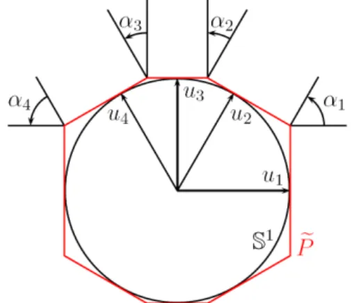
{(cosϕ,sinϕ): 0_≤ϕ<π_}and are ordered according toincreasing angles.We write<) (u,v)_∈[0,π]for the (smaller) angle between the unit vectors u and v. Letαi

be the outer angle of the vertex between the ith and the

(i+1)st edge (i.e.,αi is the angle of the normal cone

at this vertex, in other wordsπ₋αi is the usual inner

angle; see Fig. 2). Explicitly, we have

αi=

(

<) (ui,ui+1), i=1, . . . ,k−1, π−<) (u1,uk), i=k,

(16)

as the normal of the(k+1)st edge is₋u1.

Fig. 2. Construction of the anglesαi and the polytope

e

P given byEq.15 with k=4.

As the length of the ith edge of P is tane (αi/2) +

tan(αi−1/2)and S(Ze) =4, we obtain

e

Z=ec1[−u1,u1]⊕. . .⊕eck[−uk,uk],

with

e

ci=erk

tan(αi/2) +tan(αi−1/2)

2 , (17)

and

e

rk= k

∑

tan(αi/2)

!₋1

, (18)

where we have put α0 =αk. This and V(Ze) = 2erk

was also derived by Knebelman (1941). The weightsc_ei

are based on the application of Bonnesen’s inequality

Eq. 14 and will be called Bonnesen weights in the following. The ith weightceiis the relative length of the ith edge of the polygon with facet normals_±uiwhich circumscribes a circle of radiuserk. The outer radiusRke

of Z is the largest distance of a vertex ofe Z from thee

origin, and this is

e

Rk=erk k

max

i=1 1 cos(αi/2)

. (19)

Summarizing, we have shown the following. If Sb2_k(A) is an estimator of S(A)>0 given byEq. 6 with the Bonnesen weights ci =eci, i=1, . . . ,k, from Eq. 17,

then the relative errors obey

π

2erk≤ b S2_k(A)

S(A) ≤ π

2Rek. (20)

These error bounds are sharp; see Example 2.

It should be noted that Eq. 14 is always a strict inequality unless K is a disk. As Eq. 14 is used for zonotopes here, this approach will not necessarily lead to the optimal choice of the weights. However, the choice may be better than choices for the weights motivated by usual quadrature rules.

Example 3 We consider the integrand in Eq. 6 with k=3 and the directions ui = cos(ϕi),sin(ϕi)

, i=

1,2,3, where

ϕ1=0, ϕ2= π

16, ϕ3= π 8 .

As mentioned before, the rectangular quadrature rule leads to the Voronoi weights cV_i : The ith weight is the normalized length of the Voronoi arc corresponding to ui (arc inS1of all points closer to uithan to any other point in_{±u1,±u2,±u3}). This gives

cV_i = ϕi+1−ϕi−1

2π ,

where we assumed π-periodicity. For the present example, we obtain

cV =

15 32,

1 16,

15 32

,

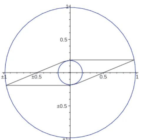
and the corresponding zonotope ZV has inradius rV _≈0.18290 and circumradius RV ≈ 0.98199; see Fig. 3. Thus, the width of the minimal annulus is approximately 0.79909.

Using instead the Bonnesen weights yields approximately

ec= (0.490 57,0.018 85,0.490 57),

leading to the inradiuser_≈0.191 412 and circumradius

e

R_≈0.981 147, respectively. The width of the minimal

annulus is now approximately 0.789 735, which is an

–1 –0.5

0.5 1

–1 –0.5 0.5 1

Fig. 3. The zonoid from Example 3 associated to Voronoi weights together with its minimal annulus.

To formulate an asymptotic result, we have to specify how close the set of the directions u1, . . . ,uk

is to a set of equidistant directions. Following Gardner

et al. (2006), we introduce the symmetrized spread∆∗_k

of u1, . . . ,uk by

∆∗ k=max

u_∈S11min_≤i_≤kmin{ku−uik,ku−(−ui)k}.

Geometrically, ∆∗_k is the maximal distance of a unit vector from the set _{±u1, . . . ,±uk}. In particular,

{±u1, . . . ,±uk} is a ∆∗k-net in S1. For αi defined by Eq.16, we have

2 sinαi 4 ≤∆

∗

k, i=1, . . . ,k. (21)

The following theorem shows that the choice ci=

e

ci leads to a relative error of Sb2k(A) that depends quadratically on∆∗_k. Here we only consider sampling sets _{u1, . . . ,uk} such that every closed sub-arc of S1 _{of length} π_{/2 contains at least one point of}

{±u1, . . . ,±uk}. Equivalently,∆∗k ≤

p

2₋√2.

Theorem 4 Let A ⊂ R2 _{be a polyconvex set with}

positive perimeter. Let k_≥2 and_{v1, . . . ,vk} ⊂R2\

{0_} such that the symmetrized spread of the vectors ui=vi/_kvi_k, i=1, . . . ,k, is∆∗_k≤p2₋√2. IfSb2_k(A)in

Eq.3 is calculated using the Bonnesen weights ci=_eci, i=1, . . . ,k, fromEq.17, then the relative error obeys

b

S2_k(A)₋S(A) S(A)

≤

π2 3 (∆

∗ k)

2_.

(22)

Proof FromEq.20 we get

πerk−2≤2 b

S2_k(A)₋S(A) S(A)

!

≤πRek−2. (23)

We estimate the left hand side ofEq. 23. In view of

Eq.21, we haveαi/2≤2 arcsin ∆∗_k/2

≤π/4 for all

i=1, . . . ,k. Taylor’s theorem implies

tan(αi/2)≤αi/2+c′(αi/2)3, for all i=1, . . . ,k,

where c′ = 8_{/3 is the third derivative of tan(x)/3!} evaluated atπ/4. Relations 18, 21 and arcsin(x)_≤π₂x,

0_≤x_≤1, imply that

πerk≥

π ∑k

i=1

αi

2

1+c′ αi

2

2≥

2

1+c′₄π2 ∆∗_k2,

and this gives

πerk−2≥ −

2π2 3 (∆

∗ k)

2

.

The right hand side ofEq. 23 can be estimated in an even easier way using the fact that the perimeter of the incircle ofZ is bounded by Se (Ze) =4 and hence

erk_≤2/π. Together withEq.19 this gives

πRek−2≤

2

1₋ ∆∗_k2(∆

∗ k)

2

≤ √2

2₋1(∆

∗ k)

2

,

as∆∗_k≤p2₋√2. Putting things together we arrive at

b

S2_k(A)₋S(A) S(A)

≤c(∆

∗ k)

2

with c=maxπ2/3,1/(√2−1) =π2/3.

Using the fact that Voronoi weights deviate only slightly from Bonnesen weights as k increases, it can be shown that the same order of convergence also holds for the relative error ofSb2_k(A)if the estimator is based on Voronoi weights. The example of equidistant sampling shows that quadratic behavior is the best possible.

Example 5 Consider the special case where u1, . . . ,uk

are equidistant on the upper half circle, meaning that ui= (cos(iπ/k),sin(iπ/k)), i=1, . . . ,k. Hence

∆∗ k=2 sin

π 4k ∼

π

2k, k→∞.

By symmetry arguments, the weights leading to the minimal width of the corresponding minimal annulus must all be equal and thus c1 =. . .=ck =1/k and

ci =eci for i=1, . . . ,k. According to Eqs.18 and 19, the inner and outer radii of the associated zonotope are

e

rk=

k tan

_π

2k

₋1

and

e

Rk=erk

cos

_π

2k

−1

=k sin

_π

2k

−1

,

cf.Eq.4. Therefore, the width of the minimal annulus is

e

Rk−erk= π 4k

−2_{+O k}−4_{, k}

→∞.

This shows that Rke ₋erk, and thus the relative worst case error, are of order ∆∗_k2.

Instead of using the above geometric arguments to obtain asymptotics for the worst case error, one might also use methods from optimum quantization (see Gruber, 2004). Among other important applications, this theory yields asymptotic minimum errors of numerical integration for classes of H¨older continuous functions. As the function gu: v7→ |hv,ui|, and hence

the function pv in Eq. 5 are Lipschitz continuous,

optimum quantization gives an upper bound for the worst case error depending linearly on ∆k. This

suboptimal rate is due to the fact that the class of H¨older continuous functions with H¨older exponent 1 is considerably larger than its subspace spanned by

gu: u∈S1 _.

A SEMI-RANDOMIZED APPROACH

The associated zonotope for quadrature rules can also be used in the context of a semi-randomized approach, which generalizes systematic random sampling designs. The idea of this design based approach is to evaluate the total projections of the randomly rotated setϑA in k directions. In other

words, given k vectors v1, . . . ,vk _∈Sd−1 _{and weights} c1, . . . ,ck, the estimator for S(A)is defined by

b

Sd_k(ϑA) = 2

γd k

∑

cip_ϑ−1_v

i, (24)

where ϑ is a random rotation whose distribution is the normalized Haar measure on the compact group

SOd of proper rotations. Clearly, Eq. 24 defines a random variable and Crofton’s formula implies that

this variable is an unbiased estimator for S(A). In particular, if d = 2 and the set _{±v1, . . . ,±vk} is equidistant in S1_{, the estimator S}bd

k(ϑA) in Eq. 24 is

the one obtained from systematic random sampling. Moran (1966) considered this special case and gave worst case bounds for the variance of Sbd_k(ϑA). His approach allows a geometric interpretation which is not restricted to the planar setting: Let Z be, again, the

zonotope associated to a fixed quadrature rule. From

Eq.11 and the unbiasedness of the estimator, we get

VarSbd_k(ϑA)=E_ϑSbd

k(ϑA)−S(A) 2

=γ−2 d Eϑ

_Z

Sd−1(hZ(ϑu)−γd)S(A,du)

2 .

Hence

Var

b

Sd_k(ϑA)=

γ−2 d

Z

Sd−1

Z

Sd−1J(u,v)S(A,du)S(A,dv), (25)

where

J(u,v) =E_ϑ((hZ(ϑ_u)−γd_{) (hZ(}ϑ_v)−γd_{)) .}

H¨older’s inequality implies that

J(u,v)_≤E_ϑ(hZ(ϑ_u)−γ_d)21/2

×E_ϑ(hZ(ϑ_v)−γ_d)21/2

=

Z

Sd−1(hZ(u)−γd)

2_µ

(du).

Hence

Var

b

Sd_k(ϑA)_≤S(A)

2

γ2

dϖd δ2

2

Z,γdBd

, (26)

where δ2(·,·) denotes the L2-metric defined earlier. This inequality is sharp, as equality holds here for example whenever A is a set of dimension d ₋ 1. The quadrature rule is exact when A = Bd and thus Sbd_k Bd= dκd, which implies that 2γd is the

mean width b(Z) of Z and γdBd is the Steiner ball of Z; see Schneider (1993, p. 353). Hence,

the coefficient of variation

r

Var

b

Sd_k(ϑA)/S(A)

is bounded from above by a multiple of the L2-distance of Z to its Steiner ball. Again, a geometric inequality (Groemer, 1990) would allow to give an upper bound of the right hand side of Ineq. 26. However, a more direct evaluation is possible and was carried out by Jan´aˇcek (2001). In particular he found optimal weights c1, . . . ,ck to minimize the variance

in the case of a “totally anisotropic object”, i.e., a set A contained in a hyperplane. The optimal weights are obtained by inverting the covariance matrix of

(p_ϑ−1_u

ERROR BOUNDS FOR DIGITAL

SURFACE AREA ESTIMATORS

In this section we consider digitizations of a

topologically regular polyconvex set A ⊂ Rd _on

rectangular grids and assume that the directionsuiare givenas normalizeddifference vectors of grid points, which usually are neigbours. For example, we consider the common 4- and 8-neighborhoods in the plane. We compute Voronoi- and Bonnesen-weights together with the associated in- and circumradii explicitly and give asymptotic error bounds forSb(A) for increasing resolution of the digitization.

To digitize A we consider the rectangular point grid G ₌ ζ₁Z _×ζ₂Z _{×. . . ×}ζd₋₁Z _×Z_{, where}

ζ1, . . . ,ζd−1>0are thegriddistances in the directions of the axes, and we used the grid distance in the last coordinate direction as unit. A grid cell is any

d-dimensional cuboid z+ [0,ζ1]×. . .×[0,ζd−1]× [0,1],z _∈ G_{. Motivated by design based stereology,}

we consider digitizations of A by a randomly translated grid. With the random variableξ, uniformly distributed in an arbitrarily chosen grid cell, the random grid ξ+G_{is a stationary random closed set}

and is called a stationary grid in Kiderlen and Rataj (2006).

In order to increase resolution, we scale the grid by a factor t>0 and denote the digitization of A in the scaled grid t(ξ+G_)by∆_{t(A). Let Q be a non-empty}

compact set, called the sampling element. We assume that each grid point x_∈t(ξ+G_{)is the center of a small}

sampling window x+tQ, which can be thought of as

a pixel or voxel. The pixel digitization consists of all grid points x for which this sampling window x+tQ

hits the set A. Hence ∆t(A) = A⊕t ˇQ

∩t(ξ+G_),

where ˇQ is the reflection of Q at the origin. For Q=_{o_} the pixel digitization reduces to the Gauss

digitization (sometimes called hit-or-miss digitization)

containing all points of the scaled grid in A. All results on error bounds in this section will be stated for the pixel digitization and therefore also hold for the Gauss digitization. In image processing, the term digitization often denotes the union of pixels (grid cells) which are centered at grid points in ∆t(A). As such pixel unions are in one-to-one correspondence with the unions of their centers, one may equivalently consider digitizations as subsets of the grid, and we will do so througout the paper.

We fix a set A and estimate its surface area S(A)

from the information available in its digitization∆t(A)

using a discretized Crofton formula; cf. Ohser and M¨ucklich (2000). We will focus on the asymptotic error of this estimator when the grid spacing gets

finer, i.e., when the digitized set ∆t(A) becomes a

better approximation of the original set A. The function

pv given by Eq. 2 can easily be estimated from

the digitized set ∆t(A) by comparing the values of

neighboring points, if v is a gridpoint. For any vector

v_∈G_{\{o}such an estimator is given by}

b pv(t) =

td−1

kv_k#{x∈t(ξ+G): x∈∆t(A),x+tv∈/∆t(A)} .

This estimator counts the number of points x in the digitized set ∆t(A) such that x+tv does not lie

in the digitization of A. From Kiderlen and Rataj (2006, Theorem 5) it follows that this estimator is asymptotically unbiased, i.e.,

lim

t_ց0

E_{pbv(t) =pv. (27)}

Having chosen k vectors v1, . . . ,vk∈Gand scalars c1, . . . ,ck≥0, one can define

b

Sd_k(A;t) = 2

γd k

∑

cibpvi(t), (28)

and it follows from Eq. 27 that Sbd_k(A;t) is an asymptotically unbiased estimator forSbd_k(A), as t _ց0. Note that the estimator given by Eq. 28 can be calculated from the knowledge of the digitization ∆t(A)of A alone.Sbd_k(A;t)behaves approximately like

a discretized Crofton integral, when t is small. Thus, the methods and resultsof the previous sectioncan be applied to obtain asymptotic error bounds.

To illustrate this approach we discretize the Crofton integral using only directions parallel to the coordinate axes: in Rd _{we choose the 2d grid points}

vi=₋vd+i=ζiei, i=1, . . . ,d−1 and vd=−v2d=ed where eidenotes the ith unit vector. Due to symmetry,

the weights leading to a minimal error interval are all equal, ci =1/(2d),i=1, . . . ,2d, and coincide with

the Voronoi weights. The zonotope Z defined in Eq.

10 is given by Z = [₋1_/d,1_/d]d _{and it has inradius}

r=1/d and circumradius R=1/√d. Lemma 1 and

the asymptotic unbiasedness ofSbd_2d(A;t)imply

1

dγd ≤

lim

t_ց0

E_Sbd

2d(A;t)

S(A) ≤

1

√

dγd .

In the planar case we haveγ2=2/πand

0.785_≈π 4 ≤limt_ց0

E_Sb2

4(A;t)

S(A) ≤

π 4

√

which means the asymptotic relative error is 21.5 % in the worst case. In three dimensions, the asymptotic relative error is at most 33.3 % asγ3=1/2 and

0.667≈2

3 ≤limtց0

E_Sb3 6(A;t)

S(A) ≤

2 3

√

3≈1.155.

Due to Stirling’s formula we have√dγd →

p

2/π as

d_→∞. As√dγd is decreasing in d, we have

0_≤lim

tց0

E_Sbd

2d(A;t)

S(A) ≤ r

π

2 ≈1.253,

for all d, where pπ/2 is the best upper bound that holdsfor arbitrary dimension d. We do not obtain a non-trivial uniform lower bound, as there are d_∈N

and sets A inRd_{with S(A) =1, but such thatS}bd

2d(A)is arbitrarily close to 0. Due to the large worst case error even in low dimensions, the above choice ofgrid points

is not recommended for practical applications. Instead, a larger number of gridpointsshould be used. On the other hand, the estimator of S(A)inEq.28 is based on asymptotic considerations and becomes less reliable when the lengths of the vectors viare large. One would

therefore restrict to vectors with bounded length, i.e., vectors contained in a small Euclidean disk around the origin. For computational reasons it is easier to replace the Euclidean disk by a disk with respect to the maximum norm.To be specific, we choose_{v1, . . . ,vk}

in the set

V_n(d)_{:= [−}ζ_1(n−1),ζ_{1(n−1)]×. . .}

×[₋ζd−1(n−1),ζd−1(n−1)]×[−(n−1),n−1]\{o}.

For n = 2, the most common choice in applications, we have

V(d)

2 ={−ζ1,0,ζ1} ×. . .

× {−ζd−1,0,ζd−1} × {−1,0,1} \ {o} , (29)

and k= #V(d)

2 =3d−1. We determine asymptotic worst case errors for n=2 and n=3 in the planar case and for n=2 in dimension d=3.

THE TWO-DIMENSIONAL CASE

In the planar case for n= 2, the k=32₋1 =

8 grid points of the set in Eq. 29 are just the 8-neighbours of the origin, and the corresponding directions are parallel to the edges and diagonals of a grid cell. Both the Voronoi weights and the Bonnesen weights can be computed analytically. It turns out that the Voronoi weights and the Bonnesen weights do not coincide, and the corresponding

in-and circumradii are different. In the following letβ =

arccos(ζ1/√ζ₁2+1). For the Voronoi case, the inradius rVor(ζ1)and the circumradiusRVor(ζ1)are given by

rVor(ζ1) =  

 1

πβ+₂√ζ_ζ12 1+1

, ifζ1≤1,

1 2−

1

πβ+₂√_ζ12 1+1

, otherwise,

and

RVor(ζ1) =

                           1 π "

β2₊

π

2−β+

π

2√ζ2 1+1

2#1/2

,

ifζ1≤1,

1

π

"

β+π_2√ζ1

ζ2 1+1

2

+ π₂₋β2 #1/2

,

otherwise,

respectively. In the Bonnesen case the inradius rBon(ζ1)is given by

rBon(ζ1) =ζ1

2 q

ζ2

1+1(ζ1+1)−2 ζ 2 1+1

−1

and the circumradiusRBon(ζ1)is given by

RBon(ζ1) =

                        

rBon(ζ1)

√

2

1+_ζ12 1

+1

₋1/2−1/2

,

ifζ1≤1

rBon(ζ1)

√

2

1+ ζ2 1+1

₋1/2−1/2

,

otherwise.

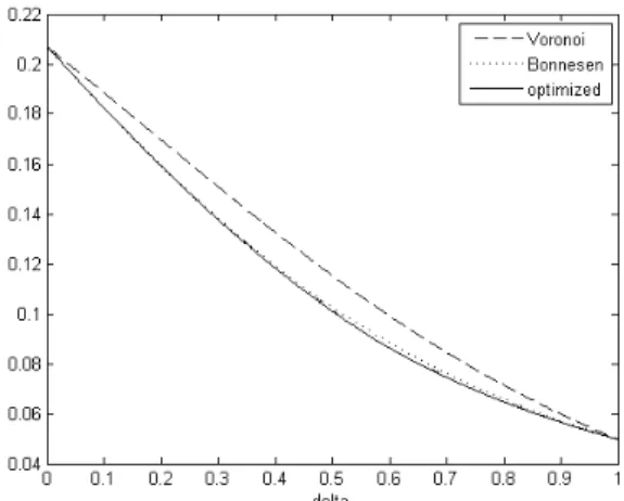
Fig. 4. Thickness of the minimal annulus for eight

directional vectors on a rectangular grid in 2D depending onζ1for Voronoi, Bonnesen, and optimized weights, respectively (see the text for details).

Fig. 5. Thickness of the minimal annulus for 16

directional vectors on a rectangular grid in 2D depending onζ1for Voronoi, Bonnesen, and optimized weights, respectively (see the text for details).

It is easy to see that in the case of a square grid (ζ1 =1) the width R−r of the minimal annulus is minimal if and only if all weights are equal, c1 = . . . = c8 = 1/8, a choice which coincides with the Voronoi and the Bonnesen weights. The corresponding zonotope Z is a regular octagon with side length 1/2 and facets parallel to the vectors v1, . . . ,v8. Z has circumradius R=p4+2√2/4 and inradius r=

1+√2/4. Withγ2=2/π we get

0.948_≈π 8

1+√2

≤lim

t_ց0

E_Sb2 8(A;t)

S(A)

≤π₈

q

4+2√2_≈1.026.

This was also obtained in Kiderlen and Jensen (2003).

We consider also the case n=3 in the plane, i.e., we use all 16 directionsobtained by normalizing the grid points in the cuboid [₋2ζ1,2ζ1]×[−2,2]\ {0}. Now even in the special case when ζ1 = 1 the 16 weights leading to a shortest asymptotic error interval are not equal. We refrain from explicitly stating the formulas for the in- and circumradii because of their complexity. The results are qualitatively similar to the case n=2. The use of the Bonnesen weights yields a smaller thickness of the minimal annulus than the use of the Voronoi weights. The minimal thickness achieved with optimized weights is only slightly better than for Bonnesen weights (Fig. 5).

THE THREE-DIMENSIONAL CASE

In three dimensions, we restrict considerations to the cubic grid (ζ1=ζ2=1) and n=2.The directions associated to the k=33₋1= 26 grid points vi of

the set in Eq. 29 consist of the 6 directions along the edges (i =1, . . . ,6), 12 diagonals of the faces (i=7, . . . ,18) and 8 spatial diagonals (i=19, . . . ,26) of the unit cube [0,1]3. Hence, the surface area estimator in Eq. 28is based on comparison of pixels with neighbors in the so-called 26-neighborhood. The Voronoi weights can be calculated as the relative sizes of the Voronoi cells on the unit sphere generated by _{v1/kv1k, . . . ,vk/kvkk} . They can be derived by computing the area of the Voronoi cells on the unit sphere analytically with the help of spherical trigonometry, and are given by

ci=                                 

1 2−

2

πarccos

_√

2+√3

√

2√3₋√3sin

π

8

≈0.045 777 9, if i=1, . . . ,6,

1 2−

1

πarccos

_√

6−2 2√3₋√6sin

π

8

≈0.036 980 6, if i=7, . . . ,18,

1 2−

3 2πarccos

(2−√3)(2−√6)+2 4√3₋√3√3₋√6

≈0.035 195 6, if i=19, . . .,26. The zonotope Z is the convex hull of all points of the form∑26_i=1εivi/kvik, where(ε1, . . . ,ε26)runs through all vectors in _{−1,0,1_}26. The quickhull-algorithm (Barber et al., 1996) was used to find this convex hull. Z has 96 vertices, inradius rVor ≈ 0.463 312, circumradius RVor _≈ 0.511 386, and thickness of minimal annulus TVor_≈0.048 074 8. As γ3=1/2 we obtainthe bounds

0.927_≤lim

tց0

E_Sb3 26(A;t)

S(A) ≤1.023.

be generalized to higher dimensions. We will do so for comparison with the established Voronoi weights. Recall the construction for the Bonnesen weights in the plane for givenvectors v1, . . . ,vk ∈R2\ {o}. We

defined ui = vi/kvik, i = 1, . . . ,k, and constructed

the polygon P ine Eq. 15 with outer unit vectors

±u1, . . . ,±uk circumscribing the unit ball. We then

chosec_eiproportional to the length of the edge ofP withe

outer unit normal ui. In higher dimensions, for given v1, . . . ,vk∈Rd\ {o}, we set ui=vi/kvik, i=1, . . . ,k,

and

e

P := k

\

i=1

n

x_∈Rd_{:|hui,xi| ≤1}o _,

in complete analogy toEq.15. HenceP is the polytopee

circumscribing the unit ball with facet normals in

{±u1, . . . ,±uk}. We then choose eci proportional to the (d₋1)-dimensional volume of the facet of Pe

which has outer unit normal ui. In the present

three-dimensional example (with ζ1=ζ2 =1 and allgrid points inV(3)

2 ) the Bonnesen weights were computed with quickhull and are given by

e

ci_≈

  

 

0.046 589 4, if i=1, . . . ,6,

0.036 743 9, if i=7, . . . ,18,

0.034 942 1, if i=19, . . .26.

The associated inradius is rBon ≈ 0.462 424, the circumradius is RBon ≈0.511 243, and thickness of minimal annulus is TBon ≈0.048 818 7. This shows that Bonnesen weights are not better than Voronoi weights for the 3d₋1 directions in dimension d=3. But this is not surprising because they are based on Bonnesen’s inequalityEq. 14 which is valid only for two-dimensional convex bodies. In the last section

we discuss how the approachdeveloped in this paper

could be extended to higher dimensions.

Finally, we show how the asymptotic relative error bounds in the case of a quadratic (ζ1=1) planar grid depend on the choice of n. To do so, the symmetrized spread of the normalized vectors of V_n(2) _{must be} determined.

Lemma 6 For n _≥ 2 the symmetrized spread of

n

x/_kx_k: x_∈V_n(2)o_{is equal to}

dn=

v u u u u

t2−

v u u u

t2



1+q n−1

1+ (n₋1)2 

_≤ 1

2(n₋1).

(30)

Proof Let∆ be the symmetrized spread of D := n

x/_kx_k: x_∈V_n(2)o _{and set m :=n−1. Clearly, the}

arc C _⊂ S1 _{in the first quadrant with endpoints} (1,0)⊤, m2+1−1/2(m,1)⊤_∈D does not contain any

other points in D and thus the spread∆is at least the distance of the midpoint of C to one of its endpoints. Hence

∆≥

r

2

1₋cosϕ 2

=

v u u

t_{2 1−}

r

1+cosϕ 2

! =dn,

where ϕ =arccos

m/√1+m2 _{is the length of C.} This interpretation of dn also shows the inequality in Eq. 30, as dn cannot be larger then half the distance

of (1,0)⊤ from (1,1/m)⊤. To show that ∆ _≤ dn, let v,v′ _{∈D two points such that the sub-arc of} S1

connecting them does not contain any other points of D. Using reflections and translations leaving Z2

invariant, we may assume that v =x/_kx_k and v′ = x′/_kx′_k where x,x′ _∈V_n(2) _{and the angles they form} with the x-axis are at mostπ/4. We refer to Fig. 6 for a sketch of the situation. The cone between the rays spanned by x and x′ cannot contain any other points of V_n(2) _{in its interior. Let y (y}′_{) denote the point in} V_n(2)_{∩ {(m,t): t≥0} with largest (smallest) second} coordinate below (above) this cone. Then the length of the arc in S1_{with endpoints v and v}′ _{is at most the}

length of the arc C′ _⊂S1 _{with endpoints y/kyk and} y′/_ky′_k. The segment[y,y′]does not contain any points of V_n(2)_{, so y and y}′ _{are distance one apart, and the} length of C′ is bounded from above by the length of

C. Here we use the fact that among all unit intervals in_n (m,t)⊤: t_≥0

o

, the interval

h

(m,0)⊤,(m,1)⊤i has the largest gnomonic projection. This gives∆≤dn, as

v and v′where arbitrary in D.

In view of Theorem 4, Lemma 6 yields an estimate for the asymptotic relative error using the Bonnesen-weights ci=eciwhenever n≥2.

Theorem 7 Let A _⊂ R2 _{be a topologically regular}

polyconvex set with positive perimeter, n _≥ 2, and ζ1 = 1. Let Sb2k(A;t) be defined by Eq. 28, where

{v1, . . . ,vk}=Vn(2) and ci =eci, i=1, . . . ,k, are the Bonnesen weights. Then the asymptotic relative mean error obeys

lim

tց0

E_Sb2

k(A;t)−S(A) S(A)

≤

π2

12(n−1)

Fig. 6. Construction to determine the symmetrized

spread in Lemma 6: the points x and x′ in V_n(2) are contained in the cube [0,n₋1]2 and their normalizations v,v′inS1_.

EXTENSION TO HIGHER

DIMENSIONS

Large parts of the present worst case analysis for quadrature rules, including the use of an associated zonotope Z, are not restricted to the two-dimensional setting. In order to find an easily accessible upper bound for the width of the minimal annulus, a joint extension of Bonnesen’s refined isoperimetric inequalities Eq. 14 and the geometric inequality of Groemer (1990) to higher dimensions (which is known) is not suitable, as it involves the surface area of Z. Instead, a strengthened version of Uhrysohn’s inequality is appropriate. It reads

b(Z) b(Bd₎

d

− Vd(Z)

Vd(Bd₎ ≥cd(Z)δ

2 2

Z,γdBd

. (31)

Here cd is an explicitly known constant, depending

on d, the mean width b(Z) of Z, and the second intrinsic volume of Z. This inequality is a special case of a whole family of geometric inequalities derived by Groemer and Schneider (1991), who also showed that it implies the Bonnesen type inequality

b(Z) b(Bd₎

d

− Vd(Z)

Vd(Bd₎≥c′d(Z) (R−r)

(d+3)/2_{. (32)}

The constant c′_d, again, depends on d, b(Z) and the second intrinsic volume of Z. For d = 2 Ineq. 32 is of the same form as Ineq. 14, but with a weaker exponent. This apparently suboptimal exponent, and the problem to determine the zonotope with given mean width which minimizes the left hand side of Eq. 32 for d>2, limits the usefulness of these inequalities for applications.

ACKNOWLEDGMENTS

We want to thank Luis Cruz-Orive, Maria Hernandez Cifre, Ilya Molchanov, and the two anonymous refereesfor their helpful comments on an earlier version of this paper. The first author’s work was partially supported by the Carlsberg foundation and the Danish Council for Strategic Research. The second author’s work was partially supported by a Marie Curie Fellowship of the European Community Programme.

REFERENCES

Barber C, Dobkin D, Huhdanpaa H (1996). The Quickhull algorithm for convex hulls. ACM Trans Math Soft 22:469–83.

Bonnesen T (1929). Probl`emes des Isop´erim`etres et des Is´epiphanes. Paris: Gauthier-Villars.

Gardner R, Kiderlen M, Milanfar P (2006). Convergence of algorithms for reconstructing convex bodies and directional measures. Ann Stat 34:1331–74.

Goodey P, Weil W (1993). Zonoids and generalizations. In: Gruber P, Wills J, eds., Handbook of Convex Geometry, vol. B. Amsterdam: Elsevier, 1297–326.

Groemer H (1990). Stability properties of geometric inequalities. Am Math Mon 97:382–94.

Groemer H, Schneider R (1991). Stability estimates for some geometric inequalities. Bull Lond Math Soc 23:67–74.

Gruber P (2004). Optimum quantization and its applications. Adv Math 186:456–97.

Jan´aˇcek J (2001). Estimating length and surface area by systematic projections. Image Anal Stereol 20 (Suppl. 1):89–94.

Kiderlen M, Jensen E (2003). Estimation of the directional measure of planar random sets by digitization. Adv Appl Probab 35:583–602.

Kiderlen M, Rataj J (2006). On infinitesimal increase of volumes of morphological transforms. Mathematika 53:103–27.

Knebelman M (1941). Two isoperimetric problems. Am Math Mon 48:623–7.

Lindel¨of L (1869). Propri´et´es g´en´erales des poly`edres qui, sous une ´etendue superficielle donn´ee, renferment le plus grand volume. Bull Acad Sci St Petersburg 14:258– 69. Math Ann (1870) 2:150-159.

Ohser J, M¨ucklich F (2000). Statistical Analysis of Microstructures in Material Science. Chichester: John Wiley & Sons.

Rataj J (2002). Determination of spherical area measure by means of dilation volumes. Math Nachr 235:143–62. Rother W, Z¨ahle M (1990). A short proof of a principal

kinematic formula and extensions. Trans Amer Math Soc 321:547–58.

Schneider R (1993). Convex Bodies: The Brunn-Minkowski Theory, vol. 44 of Encyclopedia of Mathematics and its Applications. Cambridge: Cambridge University Press. Schneider R, Weil W (1992). Integralgeometrie. Stuttgart:

Teubner.