IDENTIFYING MODULARITY STRUCTURE OF A GENETIC
NETWORK IN GENE EXPRESSION PROFILE DATA
Luigi Augugliaro
Department of Statistical and Mathematical Sciences “S. Vianelli”, University of Palermo Angelo M. Mineo
Department of Statistical and Mathematical Sciences “S. Vianelli”, University of Palermo
1. INTRODUCTION
In many medical studies, Imatinib, the first member of a new class of agents that act by specifically inhibiting a certain enzyme that is characteristic of a particular cancer cell, rather than non-specifically inhibiting and killing all rapidly dividing cells, is supposed to have a significant clinic effect on chronic myeloid leukemia (CML) in chronic phase as well as in blast crisis. However, many patients in blast crisis who are being treated with Imatinib relapse at a relatively early time, suggesting that leukemia cells tend to acquire resistance to Imatinib. So far, such innate mechanism of resistance is poorly understood, but some evidences suggest that activation of alternative oncogenic pathway may confer to CML cells a BCR-ABL protein independent survival. To understand the complex-ity of the regulation of gene expression, genetic networks have been used (Schlitt and Brazma, 2007,for more details). Genetic networks are usually constructed using proba-bilistic models such as Gaussian Graphical Models (GGMs) (Dempster, 1972; Edwards, 2000). Briefly, if we consider an undirected graph withGvertices, a Gaussian graphical model is the family of multivariate normal distributionsNG(µ,Σ), where the meanµ
2. THE DATA SET
To obtain the data, the Real-time RT-PCR amplifications were run on an ABI Prism® 7900Ht Sequence Detection System (Applied Biosystems, Foster City, CA, USA). The resulting cards were quantified separately using the SDS 2.1 software package. In the preprocessing step, genes not observed in∼75% of patients were removed by our study.
Then, using the results given in Troyanskayaet al.(2001), we used the method based on thek-nearest neighbors to estimate the missing values. For each gene with missing values, the algorithm finds theknearest neighbors using the Euclidean metric, confined to the columns for which that gene is not missing. Each candidate neighbor might be missing some of the coordinates used to calculate the distance. In this case the algorithm averages the distance from the non-missing coordinates. Having found the k-nearest neighbors for a gene, the method imputes the missing elements by averaging those (non-missing) elements of its neighbors.
Log-scale was used to stabilize the variance of the cycle threshold (Ct) values. Fi-nally, in order to remove differences due to sampling, that is differences in total RNA quantity and quality, glyceraldehyde 3-phosphate dehydrogenase (GAPD) was used as internal control gene (Livak and Schmittgen, 2001). The logCt, relativized to the en-dogenous control (∆logCt), was used for our analysis. All calculations were performed using the statistical environment R (R Development Core Team, 2009) and Biocon-ductor software (Gentlemanet al., 2004), while graphs were visualized using Graphviz software (Gansner and North, 2000).
3. CENTRAL MODULES IN AGAUSSIANGRAPHICALMODEL
In recent years, the analysis of genetic regulatory networks has received a major impetus from the huge amount of data made available by high-throughput technologies such as DNA microarrays. To better understand how genes are related to each other, graphical models are usually used. For example, Friedman (2004) proposes to use a Bayesian network and Costaet al.(2008) use Gaussian graphical model to identify pathways using gene expression data. However, these methods do not consider the modularity structure of a genetic network. To overcome this problem we propose a method based on the following two steps:
i. we use the method proposed in Schäfer and Strimmer (2005a) to estimate a GGM on a sample of patients with negative molecular response to Imatinib. To gain more insight about the estimated GGM, some of the most important centrality measures are used (Freeman, 1978);
4. GGMS IN PATIENTS WITH NEGATIVE MOLECULAR RESPONSE
4.1. Fitting a GGM
Gaussian graphical models are undirected probabilistic graphical models based on the assumption that the observed data matrixXis drawn from a multivariate normal dis-tributionNG(µ;Σ), whereGis the number of genes. To obtain a GGM, usually the following procedure is employed. From the given data, the empirical covariance matrix is computed and inverted; then the empirical partial correlationsρˆi jare computed. The distribution of|ρˆi j|is inspected, and edges(i,k)corresponding to significantly small
values of|ρˆ
i j|are removed from the graph. However, when we work with a microarray data set the number of genes (variables) exceeds the sample size: for this reason the sam-ple covariance matrix is not positive definite and cannot be inverted. To overcome this problem, we use the method proposed by Schäfer and Strimmer (2005a), namely, in the first step the estimated partial correlation coefficients are obtained using the shrinkage approach proposed by Schäfer and Strimmer (2005b). Denoted byΠthe partial correla-tion matrix, the authors propose a shrinkage estimator based on the following weighted average
˜
S=λT+ (1−λ)S, (1)
whereS is the empirical covariance matrix andT is a diagonal matrix, with elements representing the variances, supposed unequal, of the variablesXi withi =1, 2, . . . ,G. Other possible models can be used in the expression (1) (see Schäfer and Strimmer (2005b) for more details). To obtain the shrinkage estimator of Π, it is sufficient to parameterize the matrixS˜in terms of partial correlation coefficients, namely
˜si j= ˜ri j
ps i isj j
.
To estimate the shrinkage parameterλ, the authors propose an analytic result based on the Ledoit-Wolf theorem (Ledoit and Wolf, 2003).
In the second step a mixture distribution is used to address the statistical testing problem of non-zero partial correlations. Formally, we assume that the partial correla-tion coefficientsρˆi j across all edges in the network follow a mixture distribution
f( ˆρi j) =π0f0( ˆρi j,κ) + (1−π
0)f1( ˆρi j) (2)
whereπ0is the prior for the null distribution
f0( ˆρi j,κ) = (1−ρˆ2i j)
(κ−3)/2 Γ(κ/2)
π1/2Γ((κ−1)/2) (3)
(a)
(b)
The (3) is the density function of the distribution of the sample of normal correla-tion coefficients underH0 :ρi j=0. In a standard setting, the resulting degrees of free-dom areκ=N−G+1, then the sample sizeNcannot be smaller thanG. To overcome
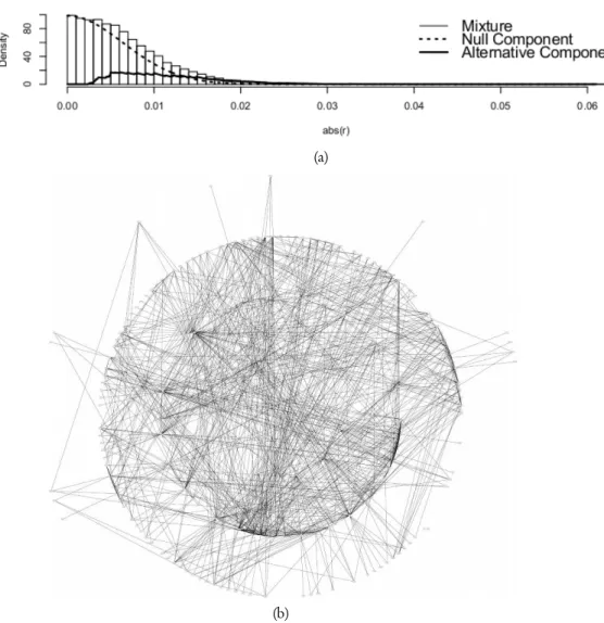
this problem, Schäfer and Strimmer (2005a) propose to estimate the degrees of freedom and the parameterπ0 fitting the mixture distribution (2) to the observed data. Using an empirical Bayesian approach, non-zero partial correlations are identified using the value 0.9 as threshold for the empirical posterior probability of an edge being present. Using a sample of 9 patients with negative molecular response to Imatinib a Gaussian graphical model consisting of 197 genes and 895 edges is obtained. In figure 1, panel (a) shows the null component and the alternative component of the mixture distribution (2), while panel (b) shows the estimated GGM in patients with negative molecular re-sponse to Imatinib. We can see that the estimated network is characterized by a high level of structural complexity. To gain more insight about the estimated relationships among the considered genes, in the following paragraph we study the estimated GGM using some of the most important centrality measures present in literature.
4.2. Central genes in a GGM
In order to gain more insight about the underlying biological processes, we evaluated the vertices (genes) of the estimated GGM using some of the most important central-ity measures (Freeman, 1978). The central genes are of particular interest because they might play the role of organizational hubs. Each centrality measure is related to a par-ticular structural attribute of the graph. The simplest centrality measure that we can compute on a given graph is thedegreeof a gene (vertex), namely, the number of genes that are adjacent to it. The second centrality measure that we have used to rank the observed genes is thebetweennessof a gene. Betweenness is useful as index of the poten-tiality of a point to control the communication within a network. Another important centrality measure that we have used in this study is theclosenessmeasure of a gene, which is related with the notion of geodesic distance on a graph, namely, the number of genes in the geodesic path joining the considered gene with another gene. Closeness of a gene is defined by the inverse of the average length of the shortest path to reach the other genes in the graph. According to the considered centrality measures, the first 10 genes (∼10% of all the genes) have been selected (table 1). Table 1 shows a key role of the
TABLE 1
Top first 10 genes obtained using the centrality measuresdegree,betweennessandcloseness. This table shows a central role of the two transcription factors EGR1 and IRF7.
Degree Betweenness Closeness
1 EGR1 EGR1 EGR1
2 IRF7 IRF7 IRF7
3 TUBA1 TUBA1 STK6
4 MGC27165 MGC27165 TUBA1
5 ADFP ADFP MGC27165
6 STK6 STK6 EPB49
7 NP CDW52 NP
8 EPB49 BCL2 TRAF5
9 BCL2 NP KLF4
10 ORC2L EPB49 ABCC4
partial correlation coefficient.
5. CENTRAL MODULES IN THE ESTIMATEDGGM
Since the estimated Gaussian graphical model is characterized by a high level of struc-tural complexity, we use the statistical approach proposed in Horvath and Dong (2008) in order to increase the comprehension of the obtained network. In the first step, we simplify the identified global network using the method proposed by Newman and Girvan (2004). Then, we use a sample of 8 patients with positive molecular response to Imatinib to identify a set of differentially expressed genes.
5.1. Finding modules
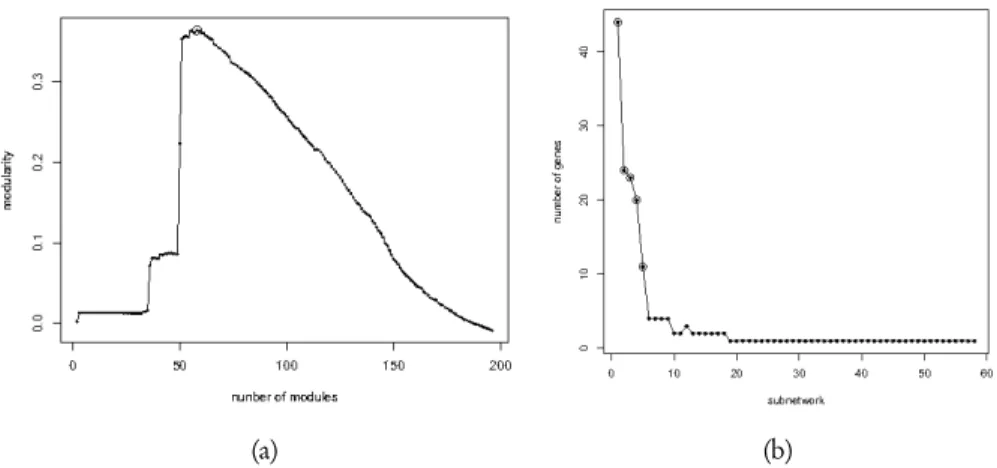
(a) (b)
Figure 2 –Panel (a) shows the modularity index as function of the number of modules identified in the estimated gene association network. The circled point corresponds to the optimal number of modules. Panel (b) shows the number of genes as function of the module ordering.
considered differentially expressed.
5.2. Central modules
In order to identify modules related with the negative molecular response to Imatinib, a sample of 8 patients with positive molecular response to Imatinib is used to iden-tify a set of differentially expressed genes. A first list of differentially expressed genes is defined combining the results obtained using the significant analysis of microarrays (SAM) proposed by Tusheret al.(2001) and the empirical Bayes analysis of microarrays (EBAM) proposed by Efronet al.(2001). In order to make this paper self-container, in this section we briefly review these methods.
SAM method is a permutation method for identifying differentially expressed genes based on a modifiedt-test statistic calledrelative distance, namely,
d(i) = ¯xn
−¯xp
si+s0 , (4)
As it is known, the false discovery rate (FDR) control is a statistical method used in multiple hypothesis testing to correct for multiple comparisons. In a list of rejected hy-potheses, FDR controls the expected proportion of incorrectly rejected null hypotheses (type I errors). In practical terms, the FDR is the expected false positive rate.
The EBAM method can be considered as a Bayesian version of the SAM method. Let π the probability that a gene is differentially expressed. We denote withEi the event that thei-th gene is differentially expressed. Let f0(d)and f1(d)be probability density functions of the test statisticd under the assumption that a gene is normal and differentially expressed, respectively. Using the mixture density
f(d) = (1−π)f0(d) +πf1(d)
and applying the Bayes’s rule, the probability that the i-th gene is differentially ex-pressed given the valuedi is computed by the following expression
P(Ei|di) =1−
(1−π)f
0(di)
f(di) . (5)
The logistic regression model is used to estimate the ratio f0(d)/f(d). To identify the differentially expressed genes, the false discovery rate can be related to the expression (5) (see Efronet al.(2001) for more details).
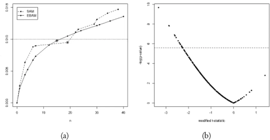
In order to make comparable the results given by the two methods, we chose 0.01 as optimal false discovery rate. Figure 3(a) shows the estimated false discovery rate as function of the number of differentially expressed genes for our data set. The highestn corresponding to an estimated false discovery rate lower than 0.01 is chosen as number of differentially expressed genes. Using this criterion, SAM leads to the identification of 19 differentially expressed genes, while EBAM leads to the identification of 16 genes, with thirteen of these that are found with the SAM. Figure 3(b) shows the results for the SAM method. The positive part of the modifiedt-statistics axis corresponds to under-expressed genes, while negative values oft-statistics indicate over-expressed genes when compared to positive molecular response. In order to obtain a good representation to discriminate between responders and non-responders, we prefer to use the−log scale
(a) (b)
Figure 3 –Panel (a) shows the plot of the estimated false discovery rate as function of the num-bernof differentially expressed genes. Dashed red line corresponds to the chosen optimal false discovery rate, while circled points correspond to the number of differentially expressed genes. Panel (b) shows the−log(p-value)as function of the modifiedt-statistics used in SAM analysis. The dashed line represents the chosen level of false discovery rate.
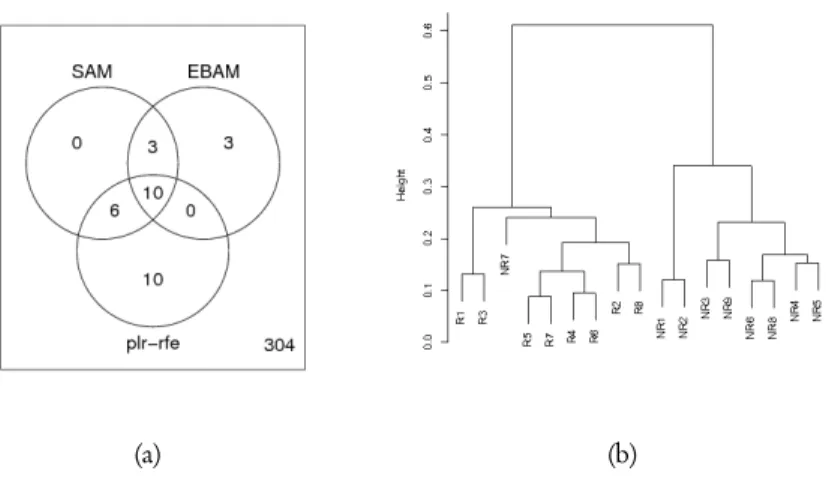
support vector machine. This iterative method is based on the univariate ranking of the genes obtained using the score function. Starting with aL2-penalized logistic regression model that includes all the considered genes, at each step the model is fitted to the data and then the gene with the smallest score function is removed from the model. This procedure is repeated until the model with the only intercept term is obtained. The final model is chosen using a cross-validation criterion. Using this method, the most accurate classifier to discriminate between responder and non-responder patients is ob-tained using a set of 26 genes, with ten of these that are included in the list previously defined. Results from SAM, EBAM and plr-rfe methods are shown by a Venn diagram in figure 4(a). If we do not consider the misclassified non-responder patients, hierarchi-cal cluster analysis shows that the other samples have good separation between the two classes, as we can see in figure 4(b). The used hierarchical clustering algorithm has been performed using the euclidean distance and the complete algorithm. The annotated gene list is shown in table 2.
(a) (b)
Figure 4 –Panel (a) shows the number of resulting genes obtained from the considered statistical methods. Panel (b) shows the results obtained using a hierarchical cluster analysis of patients with different molecular response to Imatinib. Hierarchical clustering has been performed using Euclidean distance and complete algorithm.
TABLE 2
Features of 10 genes identified as associated with negative molecular response to Imatinib.
Label Assay ID modifiedtstatistic p-value
CD34 Hs00156373_m1 −3.3351 0.0001
LYL1 Hs00245789_m1 −2.8746 0.0004
RFC2 Hs00267983_m1 −2.8669 0.0004
FVT1 Hs00179997_m1 −2.6265 0.0010
GATA2 Hs00231119_m1 −2.6248 0.0010
PEA15 Hs00269428_m1 −2.5994 0.0011
BAD Hs00188930_m1 −2.5532 0.0013
CORO1A Hs00200039_m1 −2.4640 0.0018
IRF7 Hs00242190_g1 −2.3607 0.0027
(a) (b)
(c) (d)
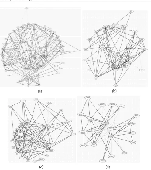
Figure 5 –Identified central modules. Continuous lines correspond to positive partial correlation coefficients, while dotted lines correspond to negative partial correlation coefficients.
of EGR1 expression (Cabodiet al., 2009). Moreover, the transcription factor EGR1, central in the module reported in figure 5(d), has been described in a recent paper as a potent tumor suppressor gene whose deregulation is involved in hematological malig-nancies (Gibbset al., 2008).
6. CONCLUSIONS
estimated model. Our method is motivated by the necessity to gain more insight about the genetic network of patients with negative response to Imatinib. The proposed framework is based on two steps: in the first step of our analysis we use a sample of patients with negative response to Imatinib to fit a Gaussian graphical model using the method proposed by Schäfer and Strimmer (2005a). Using some of the most important centrality measures (Freeman, 1978), we observe that two important transcription fac-tors play a central role within the estimated network, namely EGR1 and IRF7. In the second step of the proposed framework, we use the method proposed by Newman and Girvan (2004) to study the modularity structure of the estimated Gaussian graphical model. To identify modules that are central in our model we use a sample of patients with positive molecular response to Imatinib. A module containing a differential ex-pressed gene is defined central in the estimated model. Several identified central mod-ules are confirmed in the medical literature. Some of these interactions, like EGR1– FOXO1A are also confirmed in a recent functional study indicating that FOXO1A behaves as a negative regulator of EGR1 expression (Cabodi et al., 2009). Moreover, the transcription factor EGR1 has been described in a recent paper as a potent tumor suppressor gene whose deregulation is involved in hematological malignancies (Gibbs et al., 2008).
ACKNOWLEDGEMENTS
We want to thank Dr. Alessandra Santoro and Dr. Giuseppe Cammarata of the Hos-pital “Cervello” in Palermo for giving us the data and for their valuable explanation of the medical implications of our statistical analysis.
REFERENCES
A. L. BARABASI, Z. N. OLTVAIR(2004). Network biology: understanding the cell’s functional organization. Nature Reviews Genetics, 5, no. 2, pp. 101–113.
S. CABODI, V. MORELLO, A. MASI, R. CICCHI, C. BROGGIO, P. DISTEFANO, E. BRUNELLI, L. SILENGO, F. PAVONE, A. ARCANGELI, E. TURCO, G. TARONE, L. MORO, P. DEFILIPPI (2009). Convergence of integrins and EGF receptor signaling via PI3K/Akt/FoxO pathway in early gene Egr-1 expression. Journal of Cellular Physiology, 218, no. 2, pp. 294–303.
I. COSTA, S. ROEPCKE, C. HAFEMEISTER, A. SCHLIEP(2008).Inferring differentiation pathways from gene expression. Bioinformatics, 24, no. 13, pp. i156–i164.
A. DEMPSTER(1972).Covariance selection. Biometrics, 28, pp. 157–175.
D. EDWARDS(2000).Introduction to Graphical Modelling. Springer Verlag, New York.
B. EFRON, R. TIBSHIRANI, J. STOREY, V. TUSHER(2001).Empirical Bayes Analysis of a Microar-ray Experiment. Journal of the American Statistical Association, 96, no. 456, pp. 1151–1160. V. FERRETTI, C. POITRAS, D. BERGERON, B. COULOMBE, F. ROBERT, M. BLANCHETTE
L. FREEMAN(1978). Centrality in social networks: Conceptual clarification. Social Networks, 1, pp. 215–239.
N. FRIEDMAN(2004). Inferring cellular networks using probabilistic graphical models. Science, 303, pp. 799–805.
E. R. GANSNER, S. C. NORTH(2000).An open graph visualization system and its applications to software engineering. Software: Practice and Experience, 30, no. 11, pp. 1203–1233.
R. C. GENTLEMAN, V. J. CAREY, D. M. BATES, B. BOLSTAD, M. DETTLING, S. DUDOIT, B. ELLIS, L. GAUTIER, Y. GE, J. GENTRY, K. HORNIK, T. HOTHORN, W. HUBER, S. IACUS, R. IRIZARRY, F. LEISCH, C. LI, M. MAECHLER, A. J. ROSSINI, G. SAWITZKI, C. SMITH, G. SMYTH, L. TIERNEY, J. Y. YANG, J. ZHANG(2004). Bioconductor: open soft-ware development for computational biology and bioinformatics. Genome Biology, 5, p. R80. J. GIBBS, D. LIEBERMANN, B. HOFFMAN(2008). Egr-1 abrogates the E2F-1 block in terminal
myeloid differentiation and suppresses leukemia. Oncogene, 27, no. 1, pp. 98–106.
I. GUYON, J. WESTON, S. BARNHILL, V. VAPNIK(2002). Gene selection for cancer classification using support vector machines. Machine Learning, 46, pp. 389–422.
S. HORVATH, J. DONG(2008).Geometric Interpretation of Gene Coexpression Network Analysis. PLoS Computational Biology, 4, no. 8, p. e1000117.
O. LEDOIT, M. WOLF(2003). Improved estimation of the covariance matrix of stock returns with an application to portfolio selection. Journal of Empirical Finance, 10, pp. 603–621.
K. J. LIVAK, T. D. SCHMITTGEN(2001). Analysis of relative gene expression data using real-time quantitative PCR and the2−∆∆Ct Method
. Methods, 25, no. 4, pp. 402–408.
M. NEWMAN, M. GIRVAN(2004). Finding and evaluating community structure in networks. Physical Review, E 69, p. 026113.
R DEVELOPMENT CORE TEAM (2009). R: A Language and Environment for Statis-tical Computing. R Foundation for Statistical Computing, Vienna, Austria. URL
http://www.R-projet.org. ISBN 3-900051-07-0.
J. SCHÄFER, K. STRIMMER(2005a). An empirical Bayes approach to inferring large-scale gene association networks. Bioinformatics, 21, no. 6, pp. 754–764.
J. SCHÄFER, K. STRIMMER(2005b).A shrinkage approach to large-scale covariance matrix estima-tion and implicaestima-tions for funcestima-tional genomics. Statistical Applications in Genetics and Molecu-lar Biology, 4, no. 1(32).
T. SCHLITT, A. BRAZMA(2007).Current approaches to gene regulatory network modelling. BMC Bioinformatics, 8 (Suppl. 6).
E. SEGAL, M. SHAPIRA, A. REGEV, D. PE’ER, D. BOTSTEIN, D. KOLLER, N. FRIEDMAN (2003). Module networks: identifying regulatory modules and their condition-specific regulators from gene expression data. Nature Genetics, 34, no. 2, pp. 166–176.
V. G. TUSHER, R. TIBSHIRANI, G. CHU(2001).Significance analysis of microarrays applied to the ionizing radiation response. Proceedings of the National Academy of Sciences, 98, no. 9, pp. 5116–5121.
J. ZHU, T. HASTIE(2004). Classification of gene microarrays by penalized logistic regression. Bio-statistics, 5, no. 3, pp. 427–443.
SUMMARY
Identifying modularity structure of a genetic network in gene expression profile data
Aim of this paper is to define a new statistical framework to identify central modules in Gaussian Graphical Models (GGMs) estimated by gene expression data measured on a sample of patients with negative molecular response to Imatinib. Imatinib is a drug used to treat certain types of cancer that in many medical studies has been reported to have a significant clinic effect on chronic myeloid leukemia (CML) in chronic phase as well as in blast crisis. For central module in a GGM we intend a module containing genes that are defined differentially expressed.