Identification of Unknown Landscape Types Using CNN Transfer Learning

First of all, I would like to thank Dr. Edoardo Serra who has continuously bolstered my learning experience since the beginning of my first semester. Through continuous guidance, and uncountable productive meetings in the past two years, he has helped me identify my weaknesses and push my abilities beyond the boundaries. Dr. Serra’s passion and zeal for solving difficult problems are very influencing. Settling down with one solution has never been his choice. His critical thinking process while tackling research problems has enormously helped me understand the essence of the grueling process of scientific research, rather than just solving them. I’m very grateful to Dr. Serra not only for teaching me the application of data science and machine learning in different field of research domains, but also for helping me understand my own capabilities in tackling the problems in a most scientific way possible.

I would also like to extend my gratitude towards a bunch of great professors at Boise State University. This list includes Dr. Tim Andersen, Dr. Francesca Spezzano, Dr. Amit Jain, Dr. Sole Pera and Dr. Gaby Dagher who have influenced my learning experience through their amazing teaching abilities, respectful demeanor and continuous encouragement towards excellence. I would also like to thank my colleagues Mikel Joaristi, Axel Magnuson, Oxana Korzh and Haritha Akella for being a great support throughout my academic journey to a masters degree. All of their continuous encouragement, mentor-ship and positive attitude towards learning have

Next, I would like to thank my parents for believing in me and letting me chase my dreams. I thank them for teaching me the essence of continuous hardship, mutual respect, and courage to be patient during difficult times. I would also like to thank all my friends from Nepal for being amazing emotional support throughout this journey. There are many people who have directly and indirectly helped me learn, grow and become capable of completing my masters degree with this thesis during the past two years in and outside the Boise State University. Finally, I would like to thank everyone of them for being kind and for providing helping hands in need.

Thank you all!

Unknown image type identification is the problem of identifying unknown types of images from the set of already provided images that are considered to be known, where the known and unknown sets represent different content types. Solving this problem has a lot of security applications such as suspicious object detection during baggage scanning at airport customs, border protection via remote sensing, cancer detection, weather and disaster monitoring, etc. In this thesis, we focus on identification of unknown landscape images. This application has a huge relevance to the context of a smart nation where it can be applied to major national security tasks such as monitoring the borders or the detection of unknown and potentially dangerous landscapes in critical locations.

We propose effective semi-supervised novelty detection approaches for the un-known image type identification problem using Convolutional Neural Network (CNN) Transfer Learning. Recently, the CNN Transfer Learning approach has been very successful in various visual recognition tasks especially in cases where large training data is not available. Our main idea is to use pre-trained CNNs (i.e. already trained on large datasets like ImageNet [10]) that are then used to train new models specifically applicable to the landscape image dataset. Features extracted from these domain-specific trained CNN are then used with standard semi-supervised novelty detection algorithms like Gaussian Mixture Model, Isolation Forest, One-class Sup-port Vector Machines (SVM) and Bayesian Gaussian Mixture Models to identify the unknown landscape images.

fine-tuning approach simply uses the the class categories (landscape classes, e.g. airport, stadium, etc.) of the known images dataset. The unsupervised fine tuning approach on the other hand learns the class categories from the known images using the unsupervised clustering-based algorithm. We conducted extensive experiments that prove the effectiveness of our approaches. Our best values of AUROC and average precision scores for the identification problem are 0.96 and 0.94, respectively. In particular, we statistically prove that both fine-tuning methods significantly increase the performance of the identification with respect to the non fine-tuned CNN, and unsupervised and supervised fine tuning approaches are comparable.

ABSTRACT . . . vii

LIST OF TABLES . . . xii

LIST OF FIGURES . . . xiv

LIST OF ABBREVIATIONS . . . xvii

LIST OF SYMBOLS . . . xviii

1 Introduction . . . 1

1.1 Overview . . . 1

1.2 Contributions and Outline . . . 3

2 Background . . . 6

2.1 Supervised Learning . . . 7

2.1.1 Optimization . . . 15

2.1.2 Neural Networks . . . 17

2.1.3 Back Propagation Algorithm . . . 19

2.1.4 Convolutional Neural Networks (CNNs) . . . 21

2.2 Unsupervised Learning . . . 26

2.2.1 Novelty Detection . . . 27

2.3 Performance Metrics . . . 31

2.5 Transfer Learning . . . 34

3 Related Work . . . 37

3.1 Novelty Detection . . . 37

3.2 Convolutional Neural Networks (CNNs) . . . 41

3.3 Transfer Learning . . . 43

4 Methodology . . . 45

4.1 Baseline procedure . . . 46

4.1.1 Feature Extraction from pre-trained CNNs . . . 46

4.1.2 Novelty Detection with CNN features extraction . . . 48

4.1.3 Parameter tuning . . . 51

4.2 Novelty Detection Fine-tuning . . . 52

4.2.1 Supervised Fine-Tuning . . . 52

4.2.2 Unsupervised Fine-Tuning . . . 54

4.2.3 Clustering Ensemble . . . 56

4.2.4 Iterative unsupervised fine tuning with Novelty Detection . . . 57

5 Experiment and Result Analysis . . . 59

5.1 Datasets and Preprocessing . . . 59

5.2 Experimental Setup . . . 62

5.3 Results and Discussion . . . 65

5.3.1 Statistical Analysis . . . 69

5.3.2 Iterative unsupervised fine-tuning. . . 74

5.3.3 Autoencoder . . . 76

REFERENCES . . . 81

5.1 CNN Models with details about Fine-tuning and Feature extraction layers. . . 64 5.2 Best results for each procedure, dataset variant, and metric. . . 69 5.3 ID and description of our statistical hypotheses statements. . . 70 5.4 Table for AUROC scores: Statistical significance test table obtained by

applying statistical t-test against various combinations of experimental results. S1 (left) vs S2 (right) column represent two related sample distributions (array of scores). Third and forth columns contains mean and standard deviation of sample distributions S1 and S2 respectively. Statistical t-test has been applied according to the hypothesis as shown in HID column. Refer Table 5.3 for detailed hypothesis description.

Absolute mean difference column contains the absolute difference of mean values of sample distributions S1 and S2. p-value represents the level of significance of the comparison being done. . . 71

table obtained by applying statistical t-test against various combina-tions of experimental results. S1 (left) vs S2 (right) column represent two related sample distributions (array of scores). Third and forth columns contains mean and standard deviation of sample distributions S1 and S2 respectively. Statistical t-test has been applied according to the hypothesis as shown in HID column. Refer Table 5.3 for detailed hypothesis description. Absolute mean difference column contains the absolute difference of mean values of sample distributions S1 and S2.

p-value represents the level of significance of the comparison being done. 72 5.6 Comprehensive result table of statistical significance test with p-values

for all hypotheses as presented in Table 5.3. ** means that statistical significance level (p-value) is lower or equal to 0.01 and * means that p-value is lower or equal to 0.05. Corresponding values can also be looked up in tables 5.4 and 5.5. . . 73

2.1 Example of underfitting and overfitting when trying to fit the true distribution defined by a polynomial function with degree 4 with linear regression. (left) Underfitting case: Linear regression trained with a linear model with degree 1. (center) Optimal case: Linear regression trained with a linear model with degree 4 (right) Overfitting case: Linear regression trained with a linear model with degree 15. Source: [39] . . . 11 2.2 Overfitting and underfitting in terms of relationship between training

and generalization error. Source: [16] . . . 12 2.3 A diagram depicting a process of a single computational unit in

ar-tificial neural network analogous to the biological neuron. x0, x1, x2

are the values of a single input example,w0, w1, w2 are the parameters

associated to the input layer. P

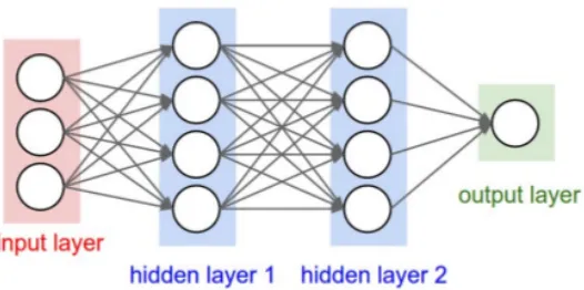
iwi, xi is a linear transformation as seen in linear models which is passed through a activation function to apply non-linear (relu, sigmoid, tanh) transformation, and is finally propagated to the next layer. Source: [23] . . . 17 2.4 A simple 3-layer fully-connected neural network with two intermediate

layers (hidden layers). This network for example can be used to learn the non-linear relationship between the input in three dimensional space that maps to a single-valued output. Source: [23] . . . 19

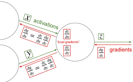
single computational unit. Note how the local gradients computed at computational unit is back propagating to previous layers by using a chain-rule of calculus. Source: [22] . . . 20 2.6 LeNet convolutional neural network architecture Source: [28] . . . 23 2.7 CNN architectures: Convolutional neural network architecture of Alexnet

model with 7 learnable layers (top) and convolutional neural network architecture of VGGNet with 19 layers (including all convolutional and pooling layers) (bottom). Source: [24] . . . 25 2.8 CNN architectures: Deep fully convolutional network architecture of

Googlenet. Source: [56] . . . 26 2.9 Simple architecture of an autoencoder with an input (Layer L1), one

hidden (Layer L2) and an output layer (Layer L3). Layer L2 captures

the embeddings of input layer into lower dimensional space. These embeddings are used by output layer to reconstruct original data. Source: [47] . . . 31 2.10 Traditional learning machine learning approach (left) and machine

learning with transfer learning (right). Source: [37] . . . 35

5.1 Examples from UC Merced Land Use (UCM) Dataset. . . 60 5.2 Examples from High-resolution Satellite Scene (HRS) Dataset. . . 60 5.3 Examples of military settlement (left) and nuclear power plant (right)

images used as unknown data classes. . . 61 5.4 Overall workflow and experimental setting for all pre-trained and

fine-tuned CNNs. . . 65

5.6 UCM with three unknown types. . . 67 5.7 HRS with two unknown types. . . 67 5.8 HRS with three unknown types. . . 68 5.9 Iteratively computed AUROC and Average Precision scores for

unsu-pervised fine tuning algorithm for (top) HRS dataset with two unknown types and (bottom) UCM dataset with two unknown types. CNN model: Googlenet. . . 75 5.10 Iteratively computed AUROC and Average Precision scores for

un-supervised fine tuning algorithm for (top) HRS dataset with three unknown types and (bottom) UCM dataset with three unknown types. CNN model: Googlenet. . . 76

CNN – Convolutional Neural Networks DNN – Deep Neural Networks

ReLU – Rectified Linearu Unit SGD– Stochastic Gradient Descent BIC – Bayesian Information Criterion

i.i.d– independent and identically distributed MSE– Mean Squared Error

GPU – Graphical Processing Units PreT – Pre-trained CNN models

SFT – Supervised Fine Tuning Approach UFT – Unsupervised Fine Tuning Approach GMM – Gaussian Mixture Models

BGMM – Bayesian Gaussian Mixture Models OCS – One-class Support Vector Machines ISOF– Isolation Forests

AUROC – Area under Receiver Operating Characteristics AVG PREC – Average Precision

Learning Rate ∇ Gradient

δ Small change (small difference)

α Level of Significance

λ Regularization parameter

CHAPTER 1

INTRODUCTION

1.1

Overview

Deep Neural Networks (DNNs), esp. Convolutional Neural Networks (CNNs)

have recently gained great success in lots of large-scale visual recognition tasks [25, 52, 56]. This has become possible because of publicly available large-scale image databases such as ImageNet (more than 14 million natural images from 20000+ different categories) [10] and powerful computing infrastructures such as GPUs and multi-node distributed clusters. In the past, ImageNet Large Scale Visual Recognition Competition (ILSVRC) has been challenging researchers around the world to develop effective and efficient visual recognition algorithms which led to the invention of deep CNNs like Alexnet [25], VGGNet [52] and GoogLeNet [56]. These CNNs achieved high and increasingly better accuracy in lots of visual recognition tasks such as image classification [36], object detection[44] and image segmentation [30].

CNNs on new and relatively smaller datasets. This particular way of transferring general feature representations from one domain (or dataset) to another is known as transfer learning. In the transfer learning context, these pre-trained models can be used either as weight initialization or as feature extractors for new datasets. Using pre-trained models as weight initialization to train the CNNs in another domain or with other datasets is generally termed as a fine-tuning approach.

Deep CNNs tend to learn general features (eg. edges and color blobs in images) on the lower level layers and more abstract and dataset specific features on the higher level layers of CNNs [63]. So CNNs can be efficiently trained on new datasets by using pre-trained models as weight initialization, freezing the learning rates of lower level layers and updating weights only for higher level layers (generally the last one or two fully connected layers). This allows the newly trained CNNs to adopt feature representations already learned from a source dataset and apply that knowledge to new datasets. This approach keeps researchers from having to train these complex CNNs from scratch thus saving a lot of computation time. CNN transfer learning approaches applied for many classification tasks have obtained accuracy scores greater than 90% for smaller training dataset and training time [36, 63].

objects in passengers’ baggage at airports are other applications that are the equally crucial security concerns that pertains to building secure and smart cities and nations. We formulate our problem as a novelty detection task to identify unknown land-scape images. We use a CNN transfer learning approach to train CNNs on two publicly available benchmark landscape datasets. We use these trained models to extract features for all known and unknown images. Features extracted from known images are used to train standard novelty detection algorithms which are finally eval-uated with test sets containing both known and unknown images using the AUROC and Average Precision metric scores.

1.2

Contributions and Outline

The main contributions of this thesis are as follows:

1. We propose the new problem of identifying unknown types of landscapes when large training sets are not available in the context of transfer learning.

2. We present an effective and efficient solution to the problem of identifying unknown type of landscape by taking in input images representing several types of known landscape. Our best AUROC and Average Precision are 0.96 and 0.94, respectively.

4. We present a supervised fine-tuning procedure which takes the categories of the known types of landscape images as input and provides outstanding performance in comparison to the baseline procedure.

5. We also present a new unsupervised fine-tuning procedure that works without any knowledge about categories of the known image examples and produces comparable results with respect to the supervised fine-tuning procedure. 6. We compare and present statistical analysis of the difference in performance

of standard novelty detection algorithms trained with features extracted from CNNs pre-trained(non fine tune tuned) and trained in supervised and unsuper-vised fine-tuning setups.

7. We collected two new categories of satellite image dataset: ’Military settlements’ and ’Nuclear power plants’. We use these two image classes as the novel (unknown) examples in our experiments.

In Chapter 2, we provide the relevant background details of machine learning in supervised and unsupervised context, neural networks and discuss commonly used standard novelty detection algorithms.

In Chapter 3, we present the literature review of previous research works re-lated to our thesis. We discuss in detail about the rere-lated works in three different topics: novelty detection, deep convolutional neural networks and transfer learning approaches.

In Chapter 5, we extend our discussion on the experimental setup, variants of experiment instances and finish up the chapter with discussion and statistical relevance about the obtained results.

CHAPTER 2

BACKGROUND

This chapter provides the relevant background on machine learning, neural networks and novelty detection algorithms. For more details on machine learning and neural networks, we recommend readers to a book by Goodfellow et al. [16]. Similarly for novelty detection algorithms, a survey paper by Pimentel et al. [42] is recommended.

2.1

Supervised Learning

Supervised machine learning is a task of searching a function from a hypothesis space given a training data with the corresponding labels. Each training example consists of independent variable(s) defining the input domain of data and dependent variable(s) defining the target. Many supervised learning can be formulated as enabling a computer to learn a function f :X →y, where X represents the space of independent variables (input space), and y the space of dependent variables (output space). To tackle any machine learning algorithms, we can almost always start by making some general design choices beforehand. Note that machine learning algorithms can be as difficult as learning very complex mathematical functions, and most of the time the most scientific way to tackle such problems is through a process: experimentation, evaluation and decision making. Here are the general design choices for building machine learning algorithms:

1. Choose the form of the model i.e. hypothesis space for candidate models

2. Choose loss function.

3. Select optimization procedure.

We introduced a couple of important machine learning terminologies above. We discuss about these design choices in the context of a simple machine learning algo-rithm, Linear Regression.

as possible. We call this process ”making a prediction” over a range of continuous values. Along the same line, classification tasks have a goal to learn a function that can achieve a prediction over a discrete class of objects. For the sake of simplicity, lets consider a case where we want to model the function mapping from two independent variables (bi-variate) to one dependent variable. Considerm observations of training data with X ∈ <2 _{and y ∈ <. We start by choosing the form of our model. The}

simplest model in this case can be a set of linear functions (F) fromX toy. A general linear model to be used as a candidate function can be formulated as:

ˆ

y=wTX+b (2.1)

where, ˆy=f(X) ∈ F is a predicted value for the corresponding input example in X, and w∈ <2 _{(= [w}

1, w2]) and b ∈ < are the parameters that define hypothesis

space. We will use the terms ”parameter” and ”weight” interchangeably in the rest of the chapter.

in linear regression setting is mean squared error (MSE) between the target and the predicted values by the candidate model.

M SEtrain =L(w)train = arg min w,b

[1/m

m

X

i=1

(wTxi+b−yi)2] (2.2)

L(w)train is also called an objective function that defines a goal of a learning algorithm to achieve the lowest possible mean squared error while achieving the best performance. Parameterswandb control the behavior of the algorithm. The weights depict the importance of each independent variable while computing the output. The higher weight value for a corresponding variable means the higher influence of this variable in determining the output. The lower weight value would result in lesser effect on the prediction.

In the real world supervised learning setting, we measure the performance of machine learning algorithms by evaluating the learned function (or model) with previously unseen observations. These observations are commonly called test data and the process of computing output for test data is termed asinference or prediction. The ability of machine learning algorithms to perform well on tasks with the test data is known as algorithm’s generalization power. How can a machine learning algorithm do well with test data when we set to observe only the training data? This is a central idea of how machine learning algorithms work and can be reasoned well with the help of statistical learning. Machine learning algorithms are developed on top of very important statistical assumption that basically says that the observations in training and test data are observed during data generating process as independent and identically distributed (i.i.d.) samples.

that aims to minimize the cost associated with each set of w and b values given the training data. The sub-expression (wTxi+b−yi)2 is the measurement of cost of this model obtained from squared difference between the true outputyi and the predicted valuewT_x

i+b. Before we discuss how to come up with the optimized parameters that minimize the cost of the function, let’s discuss common challenges pertaining to the model selection. Until now, we came to an understanding that we want to reduce the training error (prediction inaccuracy in context of regression and classification task) during the learning process. Perhaps, equally important is the ability of a learning algorithm to obtain minimum error while inferring the output for previously unseen test data. This error is commonly termed as generalization or test error.

Model complexity, Overfitting and Underfitting. In terms of mathe-matical definition, equation 2.1 is a simple model because we can describe it by using only two simple first-order coefficients ([w1, w2]) and a scalar b. Consider a

context where we are trying to find the fitting function using linear regression whose true distribution is a polynomial function with degree 4. In this case the optimal complexity of the model that we would want to use to learn this distribution would ideally be a polynomial function with degree 4.

Figure 2.1: Example of underfitting and overfitting when trying to fit the true distribution defined by a polynomial function with degree 4 with linear regression. (left) Underfitting case: Linear regression trained with a linear model with degree 1. (center) Optimal case: Linear regression trained with a linear model with degree 4 (right) Overfitting case: Linear regression trained with a linear model with degree 15. Source: [39]

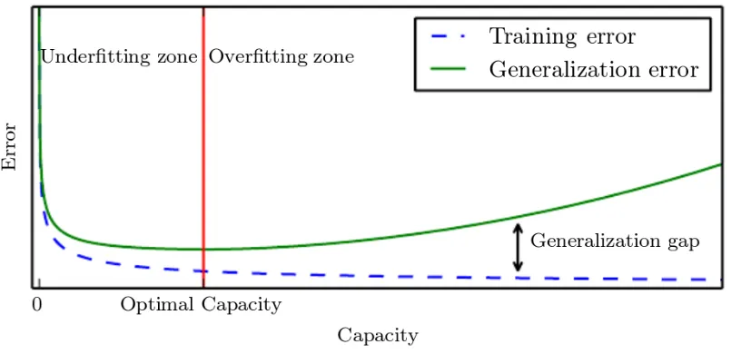
Figure 2.2: Overfitting and underfitting in terms of relationship between training and generalization error. Source: [16]

capacity or complexity to represent the underlying training data. Note: to test this mentally, imagine a point in each of the plots in the figure and compare the difference between the shortest distance of that point from the green and blue functions. Try it for all the three plots. The larger the distance, the greater the error.

In conclusion, a well performing machine learning algorithm learns from the training data with small training error during the learning phase, and also maintains the small difference between training and generalization error during the inference phase. Figure 2.2 intuitively describes all the scenario discussed above based on the choice of the model.

real world scenarios, there are cases where there might be multiple appropriate models that can equally perform well to fit the underlying data, and we should still choose a better among those models. To aid on this, and to help prevent the overfitting of the machine learning algorithms, a commonly used technique called regularization can be employed. Regularization discourages the model to learn parameters with too large values and causing one variable to have more affect on prediction than another. We can define a loss function for a linear regression problem by extending the equation 2.2 by introducing a weight decay factor as:

L(w) = arg min w,b

[1/m

m

X

i=1

(wTxi+b−yi)2] +λ(w21+w 2

2) (2.3)

where λ is a hyperparameter that penalizes the parameters and encourages the smaller values. λ = 0 means no effect of regularization and larger λ enforces smaller parameter values. In simple terms, by imposing the regularization termfw =w12+w22

(commonly used L2 norm regularizer), we are able to modify the learning algorithms not to select a model too far from the true distribution and perform well with both training and test data.

to avoid such a scenario, k-fold cross validation technique is used. Training data is divided into k equal and disjoint samples, and usually k-1 folds are used to train the model and the remaining 1 fold is used to validate. This process is repeated for k times selecting the unique validation set for each case. The final performance measure is then averaged over the k-cases hence bolstering the generalization ability of the trained models. In our work, we use 10-fold cross-validation to validate the generalizability of training of convolutional neural networks (as discussed later in this and subsequent chapters.)

Bayesian Information Criterion (BIC). When fitting models in machine learning, we discussed how we can reduce the training error (or statistically speaking increase the likelihood) by increasing or decreasing the parameters. But doing so without proper attention can also lead to a overfitting problem. Mathematically,BIC can be formulated as:

BIC =ln(m)k−2ln( ˆL) (2.4)

where, ˆ

L = the maximized value of the likelihood function of the selected model, x = training data,

m = sample size,

k = # of free parameters associated to selected model. eg. wandbin linear regression

detection task. Similar to BIC, Akaike Information Criterion (AIC) also tries to balance the trade-off between the representational power (model’s complexity) of the selected model and its ability to produce lower training error with the selected parameters. BIC has preference for simpler models compared toAIC.

2.1.1 Optimization

In the previous sections, we looked into a case where a machine learning algorithm can effectively be represented as an optimization problem. In machine learning, one of the most commonly used optimization algorithms is gradient descent. If we pose the restriction on selection of objective function to be only differentiable functions, then we can compute the gradient of the function (using numerical method or analytical method using calculus). In the neural network context, gradients are computed by using back-propagation algorithms [45] (to be discussed in detail later).

Common gradient descent operation and parameter update:

∇wL(w) = ∇w[1/m m

X

i=1

(wTxi+b−yi)2] +λ(w12+w 2

2) (2.5)

4w:=−∇wL(w) (2.6)

w:=w+4w (2.7)

gradient of L(w), ∇L(w) obtained by computing the partial derivatives w.r.t. each parameter (equations 2.5 to 2.7). The gradient descend constructs the first order approximation of Taylor expansion of L. Such gradients are used as search direction. There are different variants of gradient descend algorithm. Batch gradient descent,

Figure 2.3: A diagram depicting a process of a single computational unit in artificial neural network analogous to the biological neuron. x0, x1, x2 are the values of a

single input example, w0, w1, w2 are the parameters associated to the input layer.

P

iwi, xi is a linear transformation as seen in linear models which is passed through a activation function to apply non-linear (relu, sigmoid, tanh) transformation, and is finally propagated to the next layer. Source: [23]

2.1.2 Neural Networks

in neural networks as well. Neural networks have cascaded layered architecture. Each layer consists of computational units, generally known as neurons (from the fact that neural networks were partially inspired from biological neurons), that takes in input from the preceding layers and outputs a single valued result similar to a linear function. The computed output is then passed through a non-linear transformation (some common non-linearities used are sigmoid range(0,1), tanh range(-1,1), rectified linear unit (relu: x→max(0, x)) which is then used as input to the next layer. The process of propagating the intermediate outputs in each layer of the neural network is known as feed forward. Figure 2.3 shows the operation of one computational unit showing analogy to the operation of biological neuron. In neural networks, in addition to the design choices required to consider like in linear models, it is imperative to decide the architecture of the network we want to train for a problem at hand. The layer where the input is fed is known as input layer, the layer from where the output is fetched is known as output layer and all the other intermediate layers that perform series of linear and non-linear transformations are known as hidden layers. For example, a simple 3-layer fully-connected network is shown in Figure 2.4 which can be easily generalized to wider (more computational units in each layer) and deeper (more layers) networks. The computational units in same layers do not interact with each other and only interact with the layers immediately preceding and succeeding, making the overall computation easier to implement as matrix and vector computations. Almost all the neural network implementations are based off of efficient matrix and vector computations. And, the term deep neural network comes from using a large number of layers while designing the neural network architecture.

Figure 2.4: A simple 3-layer fully-connected neural network with two intermediate layers (hidden layers). This network for example can be used to learn the non-linear relationship between the input in three dimensional space that maps to a single-valued output. Source: [23]

each other. Then, the question is how do we compute the loss function and optimize the model parameters? Turns out, the similar representation of loss functions and same gradient-based algorithms can also be used to obtain the optimized model parameters, however with the help of back propagation algorithm which efficiently computes the gradients of neural networks. Backpropagation algorithm was formu-lated to encourage self-organizing neural networks.

2.1.3 Back Propagation Algorithm

Figure 2.5: Backpropagation of gradients through each layer shown for the case of single computational unit. Note how the local gradients computed at computational unit is back propagating to previous layers by using a chain-rule of calculus. Source: [22]

used to update the network parameters associated to each layer given the direction of the update by the gradients computed using the backpropagation. Figure 2.5 shows the propagation of local gradients through a single computational unit in backward direction of the neural network.

Summary. In general understanding, many of the concepts discussed with linear models like simple linear regression problems are generalizable to the complex machine learning algorithms like SVMs and deep neural networks as well. The design choices will vary depending upon the nature and size of training data that the considered algorithms will experience and the machine learning task to be accomplished. With neural networks, there are further decisions to be made on what type of network architecture to chose. The in-depth discussion on these topics is outside the scope of this thesis.

2.1.4 Convolutional Neural Networks (CNNs)

Figure 2.6: LeNet convolutional neural network architecture Source: [28]

functions are max−pooling, average−pooling, etc. The output of the preceding layers are fed as input to the next layer, and the output is traversed into the output layer of the network. For example in a classification problem, results of the output layer is commonly termed as logits and the operational network layers such as softmax is applied to convert logits into a probability distribution representing each number to be the probability of that input belonging to a particular category.

CNNs started gaining great attention after Krizhevsky et al. [25] won the annual ILSVRC challenge in 2012 with their breakthrough ConvNet model popularly known as AlexNet. Since then, many researchers have come up with significant improvement in the original AlexNet model (by fine-tuning the network’s hyper-parameters) or have invented many other deeper and wider networks that are best suited for various image processing and recognition tasks. In the following subsections, we discuss in detail about some standard ConvNet architecture that we will be using in our implementa-tion for training and feature extracimplementa-tion in both supervised and unsupervised setups in the later chapters.

popularly known as AlexNet. This architecture constitutes an eight layer network(five convolutional and three fully-connected). Each convolutional layer is scanned by various number of kernels (each specifically responsible to find specific features in the image), and the network tends to learn from general to more specific features as it goes into the deeper layers. Inspired from the working procedure of the human visual cortex, the size of the kernels signify the size of the receptive field in the input image to be considered for learning features specific to that particular area. Similar to the standard neural networks, units in the fully-connected layers are connected to all the units in the preceding layer. To add non-linearity to the network, this architecture uses Rectified Linear Units (ReLU)[35] as a activation function after each convolutional and fully-connected layer. This network adopts gradient descent to optimize weights in the network. ReLU adds non-saturating non-linearity in the network which is much faster than the other activation functions like tanh and sigmoid while applying gradient descent. The local response normalization used in several layers implements a form of lateral inhibition that creates competition amongst neuron outputs for important activities. This basically aids generalization on top of the non-saturating ReLUs. The pooling layers provide ways to select outputs of the neighboring neuron groups mapped by the same kernels and use a single value for a group. Alexnet uses overlapping MAX-pooling approach to select much represented value from neighborhood pixels.

Figure 2.7: CNN architectures: Convolutional neural network architecture of Alexnet model with 7 learnable layers (top) and convolutional neural network architecture of VGGNet with 19 layers (including all convolutional and pooling layers) (bottom). Source: [24]

in the forward pass and back-propagation. Meaning that, for each sample, the network randomly selects a weight shared sub-network to boost the contribution of selected subsets of neurons thus preventing overfitting and enhancing the network’s generalization power. Figure 2.7 (top) shows the architecture of 7-layered Alexnet.

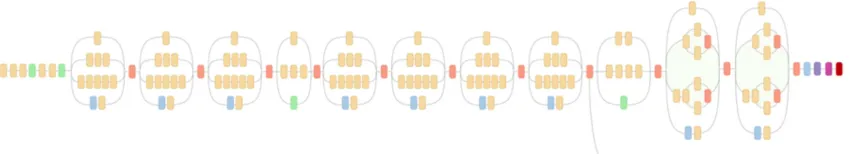
Figure 2.8: CNN architectures: Deep fully convolutional network architecture of Googlenet. Source: [56]

shows the architecture of VGGNet with 19 learnable layers.

GoogLeNet. Commonly known as inception model, Szegedy et. al [56] designed a deep convolutional neural network architecture that achieved state-of-the-art perfor-mance on image classification and detection task in the ImageNet challenge 2014. The key contribution of this architecture is the size of the learnable parameters that has 12 times fewer parameters than Alexnet, allowing the model to train in shorter time with less memory consumption. Another advantage of this model is that transfer learning using the pre-trained GoogLeNet model is much faster than Alexnet and VGGNet allowing the researchers to experiment and evaluate models in shorter amount of time. Figure 2.8 shows the architecture of fully convolutional GoogLeNet CNN.

2.2

Unsupervised Learning

2.2.1 Novelty Detection

Novelty detection is a machine learning task of identifying new or unknown data during the inference or generalization phase (test data) that were not present in the training data during the learning phase. In simple terms, the machine learning algorithm is constructed to learn the characteristics of only the ”normal” or ”known” training data. From now on, we use”normal” and ”known” interchangeably. Novelty detection algorithm expects mixtures of known and novel examples in test data during the generalization phase. By novel or unknown examples, we mean that these novel examples in test data come from different probability distribution or lies far in the feature space than the training data. We will also use the terms ”novel” and ”unknown” interchangeably as well. Novelty detection has important applications in domains involving large datasets generated from critical systems. Other applications include cyber-intrusion detection [43, 13, 62], terrorist activity, system breakdown, fraud detection [41, 59, 4, 12], data leakage prevention [51] and many other specialized applications [15].

Just to build an intuition around novelty detection algorithms, very similar classes of algorithms known asoutlier detection algorithms also have near-to-similar goals of identifying outlier or abnormal data points in the test data. The only difference is that, the unknown or abnormal instances of data points are also considered during the training phase. Outliers in dataset possess highly deviated statistical characteristics which are not in agreement with the majority of observations in the training data.

algorithms. Aiding the security applications via implementation of novelty detection algorithms in image datasets is the primary goal of our thesis. Novelty detection algorithms are commonly categorized into different categories: a) probabilistic (eg. Gaussian Mixtures), b) distance-based (eg. K-means clustering), c) domain-based (eg. one-class support vector machines), d) reconstruction-based (eg. neural networks, autoencoder) and so on. We apply Gaussian mixture models, Bayesian gaussian mixture models, one-class SVM and isolation forest (based on ensemble of trees) algorithms to apply novelty detection algorithm in our methodology. We use these algorithms to identify novel landscape images in the test data that are not present during the training phase. We will discuss in more details about the application of these algorithms specific to our application in Chapter 4. Next, we discuss in detail about how each of these algorithms can be trained to learn the normal characterstics in training phase and how to evaluate each of these models given the previously unseen test data containing both known and novel instances of data.

Gaussian Mixture Models. Gaussian mixture model is a non-bayesian, para-metric probability density based model and assumes that all the data points are gen-erated from a mixture of Gaussian distributions with unknown parameters. Gaussian Mixture model implements EM-algorithm for fitting the training data. Each sample is fitted to a probability specific to each cluster and a sample is assigned to a cluster for which it has higher probability.

Isolation Forest. Isolation forest is a model-based method that isolates unknown data points (in context of novelty detection) or anomalies (in context of anomaly detection) instead of learning profiles of the normal training data. Isolation Forest is an ensemble anomaly detection algorithm that computes anomaly score for each sample. This algorithm works by isolating observations by first randomly selecting a feature and then randomly selecting a split from a range of minimum and maximum value of the selected feature. The average depth of a tree required to isolate a sample over a forest gives the measure of normality or abnormality of that score in a distribution. Fundamentally, according to isolation forest, isolating unknown data points is easier as only few splits (fewer conditions to be checked and hence lower average tree depth) are required to distinguish the unknown data points from the known ones. In our application to identify unknown landscape images, we compute the average anomaly score of examples in test data computed from multiple random trees (base classifiers). The lower is the score for an image, the more is the data point unknown.

instances of clustering algorithm in our case) finally computing the unique consensus label for each object. In our application, we use the clustering ensemble technique to the clustering based novelty detection algorithms being used, Gaussian Mixture Model, to obtain the consensus cluster labels in order to train convolutional neural networks.

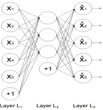
Figure 2.9: Simple architecture of an autoencoder with an input (Layer L1), one

hidden (LayerL2) and an output layer (LayerL3). LayerL2 captures the embeddings

of input layer into lower dimensional space. These embeddings are used by output layer to reconstruct original data. Source: [47]

simple 3-layered feed-forward autoencoder.

2.3

Performance Metrics

is known or novel) in order to compute Area under Receiver Operating Characterstics (AUROC) and Average Precision scores.

AUROC. AUROC score measures the discriminating ability of classifiers or novelty detection algorithms to correctly classify objects in different categories: known category and novel category in novelty detection. AUROC score basically tells how well the novelty detection algorithm is able to distinguish known objects as known and novel objects as novel in the test dataset. The AUROC is a plot with false positive rate of a discriminating model as x-axis and true positive rate in y-axis.

Average Precision. While AUROC score gives us the idea about how well the novelty detection algorithm discriminated the known and novel examples, Average Precision score on the other hand tells us the ability of novelty detection algorithm to discriminate novel objects as novel. In real world scenarios, it is common to have a very small proportion of novel examples compared to the normal examples. Therefore, we want to make sure that our novelty detection algorithms are able to discriminate the relatively small population of novel examples. False negative (eg. an unknown or security-concerned landscape image classified as known when it is unknown) rate is very critical for the discriminating models like novelty detection and we would want to lower the false negative rates as much as possible.

2.4

Statistical Significance Test

statistical empirical studies is via a statistical significance test. T-test in particular is applicable to test two related samples (eg. two different sample groups of a variable) representing some distribution. T-test is a two-sided test for the null hypothesis that two related samples have identical expected values and is commonly used with small sample sizes, testing the statistical difference between the samples. We perform t-test in following steps:

1. State the research hypothesis.

2. State the null hypothesis.

3. Select the level of significance (α)

4. Calculate test statistics value (t-value) and p-value.

5. Interpretation (make statements about the findings)

For a given two sample distributions, with sample mean ¯X and ¯Y and variance

σ2(X) andσ2(Y), respectively, we calculate the t-value as:

t value= _q X¯ −Y¯ σ2_(X)

m−1 + σ2_(Y)

n−1

where,

m =size(X)

n =size(Y)

2.5

Transfer Learning

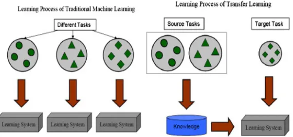
Traditional machine learning techniques have the major assumption that the training and the testing data must have the same feature space and should come from the similar (if not same) probability distribution family [37]. In many field of study, even today, it is very common to learn different new models (supervised, semi-supervised and unsupervised) even for closely related domains and problems. The common approach of building algorithms with a fixed-variated dataset as input after initial-izing a new model with zero knowledge and training those models with the popular optimization techniques do not allow the algorithm developers and practitioners to transfer prior knowledge to the related problems in similar problem domains.

Figure 2.10: Traditional learning machine learning approach (left) and machine learning with transfer learning (right). Source: [37]

Transfer learning is also closely related to the domain-adaptation. For example, if there is a news spam filtering model learned from a specific language, then if one wants to filter out the spams in the data that is the news corpus in different language or may be even with differently structured corpus (blogs, forums, etc.), then this notion of transferring the learned parameters and weights from one model to a different but related domain is called domain adaptation.

In image classification tasks where models are developed using the complex convo-lutional neural networks, in practice, very few practitioners train the whole network from scratch every-time they want to classify new set of images. Transferring weights from the the previously learned models and using those weights to extract features from the new set of images or to re-weight the newly learned model are the commonly adopted techniques that conforms to the transfer learning techniques in the field of deep neural network.

CHAPTER 3

RELATED WORK

CNNs are widely applied in image classification and segmentation tasks. Transfer learning helps to modify already trained models (pre-trained models) on large scale datasets such as ImageNet [10] in a specific application domain. In fact, using pre-trained CNNs models (usually checkpointed binary weight files) as weight initializers for training same architecture in different application domains is common in visual recognition tasks. This process is referred to as transfer learning in the context of neural networks. Recent research shows that using pre-trained models obtained by training general data followed by application-specific fine-tuning yields significant performance improvement in the image classification task [20]. In this chapter, we discuss the related works relevant to our research from all the above-mentioned fields of study.

3.1

Novelty Detection

recognition, they have employed the multi-layer perceptrons and had demonstrated the novelty detection in the context of multi-object recognition and localization of images.

Smagghe et al. in 2015 introduced the concept of local learning for multi-class novelty detection tasks [3]. Even though the results from this paper are evaluated in different benchmark image datasets, the results are very poor (AUROC in the range of 0.6). They apply nearest neighbour algorithm to select the smaller sample size to train a local multi-class novelty detection algorithm which is then used to compute the AUROC score with test data including both the known and novel dataset. Additionally, unlike this work, our work importantly focuses on feature extraction from CNNs and then applying those features with the novelty detection algorithms. The features extracted from CNNs have been proven to provide enriched representational information about the images. The paper [3] actually concludes the investigation of deep CNNs in conjunction with novelty detection algorithm to be a potential field of study.

Giacomo et al. addresses the problem of automatic novelty detection in images by training a model to represent patches belonging to the training set of normal images [5]. Basically, they consider a model based on sparse representations of images and monitor the reconstruction error to improve the detection performance using OMP algorithm. Unlike our approach, their methodology does not make use of convolutional neural networks and the highly represented features extracted from CNNs. They compute the AUROC score using very small test data and the images in their experiments are from different domain than ours.

thesis) is to identify the strict regions where the normal instances (not novel) lie in the feature space. The novelty score is given as a form of distance from these regions or sometimes as a probability that the example is not contained in any of these regions. The clustering based novelty detection techniques obtain their scores by using standard clustering algorithms such as K-Means [54] and Gaussian Mixture Models [1].

In the remaining paragraphs, we will further discuss about the application of novelty detection and outlier detection algorithms in image data that come from different type of sources. J. Theiler et al. developed an approach to identify the most unusual samples in the multispectral images. They used data attributes resampling technique to produce a background class which were then distinguished from the original dataset implementing binary classification [58]. S. Srinivasan et al. presented an approach to detect pornographic images in the internet leveraging techniques like texture analysis and face detection for non-adult content identification. They adopted techniques based on the analysis of object-level and pixel-level image contents [48]. L. Shamir et al. applied computational tools from Sloan Digital Sky Survey (SDSS) for automatic detection of peculiar galaxy pairs from the collection of nearly 400000 galaxy images. They found that the peculiar images detected by their technique involved lots of noise and weren’t actually the peculiar images and thereby concluded the paper by settling up the peculiar images by manual inspection of the detected images.

outlier detection approach which detects anomalies based on user-provided examples and a user-specified part of objects to be detected as outliers. All objects are at first mapped into a multi-granularity deviation factor (MDEF)-based feature space. This mapping is claimed to have captured the outlier-ness of the objects. The limited examples are then augmented preserving the statistical properties of the available examples and were classified using the marginal property of the SVM.

In [15], M. Goldstein et al. presented the thorough survey and evaluation of 19 different unsupervised anomaly detection algorithms on 10 different dataset from different application domains.The algorithmic performance, computational complex-ity, impact of parameter tuning and the behavior of local/global anomaly detection techniques have been studied in different setups. This paper suggests that local anomaly detection algorithms perform poorly on datasets containing global anomalies, however the global anomaly detection algorithms perform average on local problems; which suggests that it is wise to use a global anomaly detection algorithm if there is not enough information about the nature of anomaly we are dealing with on the available dataset. This paper also provides recommendation on case specific algorithmic usages. This paper, however, does not provide the use cases for image dataset and their experimental evaluations do not consider high dimensional feature set as well. V Hodge et al. also presented the extensive overview of outlier detection techniques developed in machine learning and statistics [19]. Many other similar surveys [40] were specifically focused towards particular sub-domain of the existing researches. M. Markou et al. presented the extensive study of neural network based [32] and statistics based [31] novelty detection techniques.

K. Koonsanit et. al presented a method1 _{for automatically estimating the outlier}

regions in unlabeled datasets. Their data mining algorithm implements co-occurence matrix techniques to determine outlier regions in highly pixelated satellite images. The co-occurrence matrix is first used to estimate the number of clusters, which is followed by a step that implements a standard clustering algorithm which dis-criminates outlier regions by automatic thresholding. Finally the outlier regions are depicted as indicated by the values less then some threshold. I. Delibalta et al. in [9] presented an online outlier detection algorithm applied on sequential dataset. The algorithm first constructs a score function and then fits a model to the observed data. This score is then used to evaluate newly seen observations. They constructed score function with adaptive nested decision trees. The original data space is partitioned with the nested soft decision trees in a hierarchical manner and an adaptive approach is used to mitigate overfitting issues.

There has been a large increment in the volume of satellite images (the Earth Science data) over the recent years [2]. Analysis of such large and dynamic images is very challenging because of distributed storage across the geographical locations. K. Bhaduri et al. presented the outlier identifying algorithm that is operated in almost fully distributed manner - only less than 5% of the images were needed to be analyzed in a centralized manner. Vertical data partition and specialized pruning rule resulted in higher accuracy, maintaining a low communication cost while processing a terabytes of data.

3.2

Convolutional Neural Networks (CNNs)

The main procedure was based on extracting vectors of features from an already pre-trained convolutional neural network (AlexNet without its fully connected layers) and use these vectors as input for a Gaussian classifier. In this work the authors state that the features extracted directly from the pre-trained neural network are in general representative enough and there is no need to fine-tune the pre-trained network to improve them. In this thesis we, however, show that fine-tuning the convolutional neural networks (in supervervised and unsupervised setups) improves the performance over the use of only pre-trained models (without fine-tuning).

3.3

Transfer Learning

In this section, we discuss some pioneering literature on state-of-the-art approaches on transfer learning that have been successful specifically in the field of deep neural networks and computer vision.

In many deep neural networks, selection of filters (aka kernels) and generated feature descriptors over each layer of the network in many competition winning CNN models exhibit exciting characteristics. In first few layers, CNNs tend to learn features like Gabor filters, edges and color blobs which are general properties that most of the natural images possess. In the later layers, these CNNs tend to learn more specific features associated with the particular data that the network is being trained on. J. Yosinki et al. investigated transferability of features learned from a source task to target task and they found that feature transfer has almost always a boosting effect in target domain even when the source and target tasks are distant in terms of their applicability [63]. However, practitioners should always be cautious about the drawback of negative transfer learning.

A. Razavian et al. presented a series of experiments based on several recog-nition tasks using the CNN model, OverFeat [49], investigated transfer of generic descriptors from the CNNs in range of dataset, and concluded that the the features extracted from these CNNs are indeed the most representative descriptors of the images and suggested that these features be used in most visual recognition tasks [50]. J. Donahue et al. released an open source project, DeCAF, that implements the deep convolutional activation features that have sufficient representational power and generalization ability due to transfer learning [11].

neural network to other neural networks, which eventually accelerates the training task of the significantly larger neural networks. While working with the large scale data in a neural network, researchers spend time training and experimenting with a lot of networks, of which many are a waste. The authors presented two Net2Net methodologies that are based on the function-preserving transformations: in both wider (more units in hidden layers) and deeper (more hidden layers) target neural networks. The smaller networks were trained and the knowledge stored in such networks were acquired for the initialization of the larger networks.

Z. Tang et al. used transfer learning to train Recurrent Neural Network (RNN) using the knowledge already trained from the DNNs [57]. The investigation showed that transfer learning boosts the training performance of target domain even when the source domain has the lower representational power even with the limited training dataset. DNNs are assumed to be weaker than RNNs

CHAPTER 4

METHODOLOGY

In this chapter, we discuss in detail the algorithmic implementation of convolutional neural networks and novelty detection algorithms in supervised and unsupervised learning context. Just to recap the goal of our thesis, following is the methodological outline

Problem Definition. We define the problem of identifying unknown landscape image as novelty detection task. Given the multiple types of landscape images as training experiences to the novelty detection algorithms, we want to investigate how well our novelty detection algorithms perform in detecting unknown landscape images given the combination of known and unknown landscape images (test data) not seen during the training session. Thus we say that our applied machine learning algorithms experience landscape images in both training and test session and evaluate the performance in terms of novelty score with test data. We use ”test phase” and ”scoring phase” interchangeably in this chapter.

supervised and unsupervised learning contexts.

4.1

Baseline procedure

A baseline procedure that can be used for unknown landscape type identification with transfer learning is to extract feature representations from pre-trained convolutional neural network models (already trained with large dataset like ImageNet [10]) and use these features (vector of real values) to train and evaluate standard novelty detection algorithm.

4.1.1 Feature Extraction from pre-trained CNNs

the CNNs) publicly available for other researchers to use in other relevant tasks. For example, the deep learning library Caffe [21] has it’s model zoo from where we can obtain these pre-trained models and apply these quickly as feature extractors in just a couple of minutes. In this thesis, we use three pre-trained CNN models

Alexnet [25], VGG19 [52] andGoogLeNet [56] obtained from the Caffe library. Like every other neural network, convolutional neural networks also have hierarchical and layered-based network architecture. The raw input images are fed from the lowest input layer and the network successively learns from general (eg. edges, color blobs) to more abstract (eg. football stadium, river, airport etc) concepts in images through a hierarchical representational learning process. The pre-trained models that we are using in our implementation were all trained originally on millions of natural images over more than twenty thousand categories for multi-class classification tasks and these models have learned very general features (applicable to nearly any type of existing images) in the lower layers. Since our landscape dataset is very small in comparison to ImageNet, we were able to extract rich features for our landscape images even from the higher-level layers (fully connected layers on the output end). Usually, once these CNNs are used to convert the original images(raw landscape images in our case) into a set of meaningful features, these features can be then used to train a new classifiers such as linear SVM applied to a new task which the original CNN models were not trained for. This is one of the commonly employed and simplest forms of transfer learning in context of convolutional neural networks in visual recognition.

algorithms. We describe the details of novelty detection algorithm with CNN feature extraction in next section.

4.1.2 Novelty Detection with CNN features extraction

Novelty detection as described in [42] is the task of detecting data that differs in some respect from the data that is available during training. By definition, novelties (or unknown observations) are not present in the training set and appear only on the test set. In order to identify unknown types of landscape, we define a novel example in our application domain, i.e. a type of landscape that is novel from those present in the training set (see [33]). In this thesis, we consider four commonly used effective novelty detection algorithms: (i) Gaussian Mixture Models, (ii) Bayesian Gaussian Mixture Models, (iii) One-class Support Vector Machines and (iv) Isolation Forests. Please refer to Chapter 2.2, [18] and [33] for a detailed description of each one of these methods. Implementation of novelty detection involves taking the extracted feature representation from CNN models as input, train each of these novelty detection algorithms using known landscape image samples (datasets detail and data preparation is explained Chapter 5) as training data and finally compute the novelty score for the landscape images in test data. These novelty detection algorithms return as output a score specifying the degree of novelty for each of the landscape images in the test data 1_{. We describe our novelty detection procedure in}

algorithm 1.

Algorithm 1 takes in input a pre-trained CNN modelN s.t. its last layer is exactly the one that we decide to extract the features from. In addition, we also input two set 1_{if the score is the belonging degree to the training set, the novelty score can be easily obtained}

Algorithm 1 Novelty Detection with CCN feature extraction.

1: procedure ND(N, IM Gs, T estIM Gs)

Input:N is the pre-trained (or fine-tuned) model for feature extraction,IM Gsis a set of known images that will be used as a training set to train novelty detection algorithms, andT estIM Gsis the set of images (both known and unknown types) where our procedure will search for type of unknown landscape w.r.t. IM Gs. Output: score is the novelty score for each image in test set (T estIM Gs). Trainig session

2: F eats← getFeatures(N, IM Gs)

3: for (i= 1 to k)do

4: mi ← trainNovelDetectModel(F eats)

5: end for

Scoring session

6: testF eats← getFeatures(N, T estIM Gs)

7: for (i= 1 to k)do

8: scorei ← getScore(m, testF eats)

9: end for

10: score=

Pk i=1scorei

k

11: return score

of images: IM Gs is the set of known types of landscape images used as training and

T estIM Gsis the set of images where we want to find the unknown type of landscape. The output of this procedure is a score for each image inT estIM Gs. This score tells us how much the landscape type in this image is unknown. The procedure is divided in two parts: Training session and Scoring session. The Training session consists of two main tasks: first it extracts the training features, these training features are obtained by running the training images inIM Gs through the CNNN, and second uses these extracted features to train the novelty modelsm. We train all four novelty detection algorithms using these extracted features. After the novelty detection models m are trained we proceed with the Scoring session. The Scoring session is responsible for extracting the test features from the the images in T estIM Gs, these features are again extracted using the CNN N, and scoring them with the trained novelty model

m. Usually, all the standard novelty detection procedures are subjected to random choice. This make models unstable, meaning that different runs of the procedure can obtain different models (line 4), and scores. To overcome this issue and try to get a more stable result, we decided to execute the training procedure of the novelty detection model m k times (line 3). Once the m1, . . . , mk models are obtained, we score each training image in T estIM Gs with each one of the trained models and average the produced scores (line 10) to obtain a unique ensemble score.

4.1.3 Parameter tuning

4.2

Novelty Detection Fine-tuning

One more sophisticated way to perform transfer learning in context of CNNs is by fine-tuning these CNNs. This procedure consists of refining the network (training it again) with the new specific dataset by continuing with the training checkpoint models that were initially used to train large scale natural dataset (in our case ImageNet). The fine-tuning is usually related to classification tasks. In this section we show how to fine-tune a network in the context of novelty detection. Once the network is fine-tuned, the baseline procedure can be applied. In the following sections we discuss two fine-tuning procedures, one more restrictive called supervised fine-tuning and the more general unsupervised fine-tuning procedure.

4.2.1 Supervised Fine-Tuning

Usually fine-tuning is performed in standard classification tasks where it is possible to provide examples of the new classes (at least two different classes) that the CNN is going to classify. In the novelty detection problem, only the known type of classes are available in the training, i.e. in our case only the known type of landscape. In order to perform the standard fine-tuning, we assume that our images belong to a set of disjointed categories that are all the different types of known landscape. Algorithm 2 describes our supervised fine-tuning procedure. This procedure takes in input a CNN

N to fine-tune, a set of known images to be used as training set during fine-tuning, and a set of classesC pertaining to all the images inIM Gsrepresenting specific type of known landscape. Note that the last layer of the input CNNN is exactly the layer chosen for the feature extraction.

set C (line 2). Second a new fully connected layer is added to the last layer of the CNN N. The number of neurons of this new layer is equal to n (number of distinct classes). In the third step the T rain method is applied to fine-tune the CNN on the new dataset (i.e. landscape image dataset) (line 4). The learning rate for the

T rain(gradient descend) method in the fine-tuning procedure usually decreases with the layer number that we are re-tuning. Usually the last layers have a learning rate coefficient bigger than the ones earlier in network layer. This is similar to freezing the earlier weight layers and training only the last layer. The motivation is that we want to operate a transfer learning procedure that moderately changes the weights by keeping most of the previously learned weights unaltered. In particular, the initial layers (near to input end) should have lower change because they mostly represent general features related to all natural images by itself (e.g. edges, color blobs etc.) while the higher level layers (near to output end) - the last fully connected layer in our case - should be learned more in order to allow the training process to learn features specific of the new application context (e.g. landscape images in our case). Finally, the added layer is removed and the procedure returns the new fine-tuned network that is further applied for feature extraction and novelty detection using the baseline procedure.

Algorithm 2 Supervised Fine-Tuning procedure.

1: procedure fineTune(N,IM Gs,C )

Input: N is the CNN model to be used as weight initializer, IM Gs the set of known images to be used as training data, and C is a vector the classes (labels) for each image inIM Gs to be used for supervised fine-tuning.

Output: N F fine-tuned network (i.e. after transfer learning).

2: n ←getNumberOfClasses(C)

3: N F ← addFullyConnectedLayer(N, n)

4: N F ← _Train(N F, IM Gs, C)

5: N F ← removeLastLayer(N F)

6: return N F

7: end procedure

to recognize unknown landscapes, e.g. landscapes that are somehow a combination of the known ones will tend more to be considered unknown. In the experiments, in Section 5.3 we observe this phenomena.

Since the fine-tuning approach requires us to have the information of these classes, we call this procedure supervised fine-tuning. Unfortunately, providing the type of landscape of each known image can represent a big limitation. In the next section, we will provide completely new unsupervised fine-tuning procedure that does not need the class type information in input.

4.2.2 Unsupervised Fine-Tuning

In real world scenarios, it is usually difficult to obtain the categorization (classes) information of the known images. In this section, we provide an unsupervised proce-dure that groups similar images in base to the structure of the features extracted from the CNN. We use a clusterization procedure performed by a Gaussian Mixture Model

2 _{that as a result associates each image to a cluster. Then, we use each cluster as a}

2_{Gaussian Mixture Model is a distance-based, probabilistic and parametric clustering approach}