Breaking the Curse of Kernelization: Budgeted Stochastic Gradient
Descent for Large-Scale SVM Training
Zhuang Wang∗ [email protected]
Corporate Technology Siemens Corporation 755 College Road East Princeton, NJ 08540, USA
Koby Crammer [email protected]
Department of Electrical Engineering The Technion
Mayer Bldg Haifa, 32000, Israel
Slobodan Vucetic [email protected]
Department of Computer and Information Sciences Temple University
1805 N Broad Street Philadelphia, PA 19122, USA
Editor: Tong Zhang
Abstract
Online algorithms that process one example at a time are advantageous when dealing with very large data or with data streams. Stochastic Gradient Descent (SGD) is such an algorithm and it is an attractive choice for online Support Vector Machine (SVM) training due to its simplicity and effectiveness. When equipped with kernel functions, similarly to other SVM learning algorithms, SGD is susceptible to the curse of kernel-ization that causes unbounded linear growth in model size and update time with data size. This may render SGD inapplicable to large data sets. We address this issue by presenting a class of Budgeted SGD (BSGD) algorithms for large-scale kernel SVM training which have constant space and constant time complexity per update. Specifically, BSGD keeps the number of support vectors bounded during training through several budget maintenance strategies. We treat the budget maintenance as a source of the gradient error, and show that the gap between the BSGD and the optimal SVM solutions depends on the model degradation due to budget maintenance. To minimize the gap, we study greedy budget maintenance methods based on removal, projection, and merging of support vectors. We propose budgeted versions of several popular online SVM algorithms that belong to the SGD family. We further derive BSGD algorithms for multi-class SVM training. Comprehensive empirical results show that BSGD achieves higher accuracy than the state-of-the-art budgeted online algorithms and comparable to non-budget algorithms, while achieving impressive computational effi-ciency both in time and space during training and prediction.
Keywords: SVM, large-scale learning, online learning, stochastic gradient descent, kernel methods
1. Introduction
Computational complexity of machine learning algorithms becomes a limiting factor when one is faced with very large amounts of data. In an environment where new large scale problems are emerging in various disciplines and pervasive computing applications are becoming common, there is a real need for machine learning algorithms that are able to process increasing amounts of data efficiently. Recent advances in
scale learning resulted in many algorithms for training SVMs (Cortes and Vapnik, 1995) using large data (Vishwanathan et al., 2003; Zhang, 2004; Bordes et al., 2005; Tsang et al., 2005; Joachims, 2006; Hsieh et al., 2008; Bordes et al., 2009; Zhu et al., 2009; Teo et al., 2010; Chang et al., 2010b; Sonnenburg and Franc, 2010; Yu et al., 2010; Shalev-Shwartz et al., 2011). However, while most of these algorithms focus on linear classification problems, the area of large-scale kernel SVM training remains less explored. SimpleSVM (Vishwanathan et al., 2003), LASVM (Bordes et al., 2005), CVM (Tsang et al., 2005) and parallel SVMs (Zhu et al., 2009) are among the few successful attempts to train kernel SVM from large data. However, these algorithms do not bound the model size and, as a result, they typically have quadratic training time in the number of training examples. This limits their practical use on large-scale data sets.
A promising avenue to SVM training from large data sets and from data streams is to use online algo-rithms. Online algorithms operate by repetitively receiving a labeled example, adjusting the model parame-ters, and discarding the example. This is opposed to offline algorithms where the whole collection of training examples is at hand and training is accomplished by batch learning. SGD is a recently popularized approach (Shalev-Shwartz et al., 2011) that can be used for online training of SVM, where the objective is cast as an unconstrained optimization problem. Such algorithms proceed by iteratively receiving a labeled example and updating the model weights through gradient decent over the corresponding instantaneous objective func-tion. It was shown that SGD converges toward the optimal SVM solution as the number of examples grows (Shalev-Shwartz et al., 2011). In its original non-kernelized form SGD has constant update time and constant space.
To solve nonlinear classification problems, SGD and related algorithms, including the original perceptron (Rosenblatt, 1958), can be easily kernelized combined with Mercer kernels, resulting in prediction models that require storage of a subset of observed examples, called the Support Vectors (SVs).1While kernelization allows solving highly nonlinear problems, it also introduces heavy computational burden. The main reason is that on noisy data the number of SVs tends to grow with the number of training examples. In addition to the danger of exceeding the physical memory, this also implies a linear growth in both model update and prediction time with data size. We refer to this property of kernel online algorithms as the curse of kernelization. To solve the problem, budgeted online SVM algorithms (Crammer et al., 2004) that limit the number of SVs were proposed to bound the number of SVs. In practice, the assigned budget depends on the specific application requirements, such as memory limitations, processing speed, or data throughput.
In this paper we study a class of BSGD algorithms for online training of kernel SVM. The main con-tributions of this paper are as follows. First, we propose a budgeted version of the kernelized SGD for SVM that has constant update time and constant space. This is achieved by controlling the number of SVs through one of the several budget maintenance strategies. We study the impact of budget maintenance on SGD optimization and show that, in the limit, the gap between the loss of BSGD and the loss of the optimal solution is upper-bounded by the average model degradation induced by budget maintenance. Second, we develop a multi-class version of BSGD based on the multi-class SVM formulation by Crammer and Singer (2001). The resulting multi-class BSGD has similar algorithmic structure as its binary relative and inherits its theoretical properties. Having shown that the quality of BSGD directly depends on the quality of budget maintenance, our final contribution is exploring computationally efficient methods to maintain an accurate low-budget classifier. In this work we consider three major budget maintenance strategies: removal, projec-tion, and merging. In case of removal, we show that it is optimal to remove the smallest SV. Then, we show that optimal projection of one SV to the remaining ones is achieved by minimizing the accumulated loss of multiple sub-problems for each class, which extends the results by Csat´o and Opper (2001), Engel et al. (2002) and Orabona et al. (2009) to the multi-class setting. In case of merging, when Gaussian kernel is used, we show that the new SV is always on the line connecting two merged SVs, which generalizes the result by Nguyen and Ho (2005) to the multi-class setting. Both space and update time of BSGD scale quadratically with the budget size when projection is used and linearly when merging or removal are used. We show
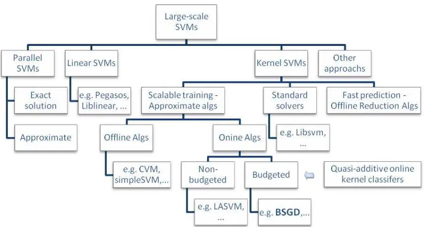
Figure 1: A hierarchy of large-scale SVMs
imentally that BSGD with merging is the most attractive because it is computationally efficient and results in highly accurate classifiers.
The structure of the paper is as follows: related work is given in Section 2; a framework for the proposed algorithms is presented in Section 3; the impact of budget maintenance on SGD optimization is studied in Section 4, which motivates the budget maintenance strategies that are presented in Section 6; the extension to the multi-class setting is described in Section 5; in Section 7, the proposed algorithms are comprehensively evaluated; and, finally, the paper is concluded in Section 8.
2. Related Work
In this section we summarize related work to ours. Figure 1 provides a view at the hierarchy of large-scale SVM training algorithms discussed below.
2.1 Algorithms for Large-Scale SVM Training
Recent research in large-scale linear SVM resulted in many successful algorithms (Zhang, 2004; Joachims, 2006; Shalev-Shwartz et al., 2011; Hsieh et al., 2008; Bordes et al., 2009; Teo et al., 2010) with an impressive scalability and able to train with millions of examples in a matter of minutes on standard PCs. Recently, linear SVM algorithms have been employed for nonlinear classification by explicitly expressing the feature space as a set of attributes and training a linear SVM on the transformed data set (Rahimi and Rahimi, 2007; Sonnen-burg and Franc, 2010; Yu et al., 2010). However, this type of approaches is only applicable with special types of kernels (e.g., the low degree polynomial kernels, string kernels or shift invariant kernels) or on very sparse or low dimensional data sets. More recently, Zhang et al. (2012) proposed a low-rank linearization approach that is general to any PSD kernel. The proposed algorithm LLSVM transforms a non-linear SVM to a linear one via an approximate empirical kernel map computed from low-rank approximation of kernel matrices. Taking an advantage of the fast training of linear classifiers, Wang et al. (2011) proposed to use multiple linear classifiers to capture non-linear concepts. A common property of the above linear-classifier-based al-gorithms is that they usually have low space footprint and are initially designed for offline learning but can also be easily converted to online algorithms by accepting a slight decrease in accuracy. Recent research in training large-scale SVM with the popular Gaussian kernel focuses on parallelizing training on multiple cores or machines. Either optimal (e.g., Graf et al., 2005) or approximate (e.g., Zhu et al., 2009) solutions can be obtained by this type of methods. Other attempts to large-scale kernel SVM learning include a method that modifies the SVM loss function (Collobert et al., 2006), preprocessing methods such as pre-clustering and training on the high-quality summarized data (Li et al., 2007), and a method (Chang et al., 2010a) that decomposes data space and trains multiple SVMs on the decomposed regions.
2.2 Algorithms for SVM Model Reduction
SVM classifier can be thought of as composed of a subset of training examples known as SVs, whose number typically grows linearly with the number of training examples on noisy data (Steinwart, 2003). Bounding the space complexity of SVM classifiers has been an active research since the early days of SVM. SVM reduced set methods (Burges, 1996; Sch¨olkopf et al., 1999) start by training a standard SVM on the complete data and then find a sparse approximation by minimizing Euclidean distance between the original and the approximated SVM. A limitation of reduced set methods is that they require training a full-scale SVM, which can be computationally infeasible on large data. Another line of work (Lee and Mangasarian, 2001; Wu et al., 2005; Dekel and Singer, 2006) is to directly train a reduced classifier from scratch by reformulating the optimization problem. The basic idea is to train SVM with minimal risk on the complete data under a constraint that the model weights are spanned by a small number of examples. A similar method to build reduced SVM classifier based on forward selection was proposed by Keerthi et al. (2006). This method proceeds in an iterative fashion that greedily selects an example to be added to the model so that the risk on the complete data is decreased the most. Although SVM reduction methods can generate a classifier with a fixed size, they require multiple passes over training data. As such, they can be infeasible for online learning.
2.3 Online Algorithms for SVM
Online SVM algorithms were proposed to incrementally update the model weights upon receiving a single example. IDSVM (Cauwenberghs and Poggio, 2000) maintains the optimal SVM solution on all previously seen examples throughout the whole training process by using matrix manipulation to incrementally update the KKT conditions. The high computational cost due to the desire to guarantee an optimum makes it less practical for large-scale learning. As an alternative, LASVM (Bordes et al., 2005) was proposed to trade the optimality with scalability by using an SMO like procedure to incrementally update the model. However, LASVM still does not bound the number of SVs and a potential unlimited growth in their number limits its use for truly large learning tasks. Both IDSVM and LASVM solve SVM optimization by casting it as a QP problem and working on the KKT conditions.
problem and model weights are updated through gradient decent over an instantaneous objective function. Pegasos (Shalev-Shwartz et al., 2011) is an improved stochastic gradient method, by employing a more aggressively decreasing learning rate and projection. Iterative nature of stochastic gradient makes it suitable for online SVM training. In practice, it is often run in epochs, by scanning the data several times to achieve a convergence to the optimal solution. Recently, Bordes et al. (2009) explored the use of 2nd order information to calculate the gradient in the SGD algorithms. Although the SGD-based methods show impressive training speed for linear SVMs, when equipped with kernel functions, they suffer from the curse of kernelization.
TVM (Wang and Vucetic, 2010b) is a recently proposed budgeted online SVM algorithm which has constant update time and constant space. The basic idea of TVM is to upper bound the number of SVs during the whole learning process. Examples kept in memory (called prototypes) are used both as SVs and as summaries of local data distribution. This has been achieved by positioning the prototypes near the decision boundary, which is the most informative region of the input space. An optimal SVM solution is guaranteed over the set of prototypes at any time. Upon removal or addition of a prototype, IDSVM is employed to update its model.
2.4 Budgeted Quasi-additive Online Algorithms
The Perceptron (Rosenblatt, 1958) is a well-known online algorithm which is updated by simply adding misclassified examples to the model weights. Perceptron belongs to a wider class of quasi-additive online algorithms that updates a model in a greedy manner by using only the last observed example. Popular recent members of this family of algorithms include ALMA (Gentile, 2001), ROMMA (Li and Long, 2002), MIRA (Crammer and Singer, 2003), PA (Crammer et al., 2006), ILK (Cheng et al., 2007), the SGD based algorithms (Kivinen et al., 2002; Zhang, 2004; Shalev-Shwartz et al., 2011), and the Greedy Projection algorithm (Zinke-vich, 2003). These algorithms are straightforwardly kernelized. To prevent the curse of kernelization, several budget maintenance strategies for the kernel perceptron have been proposed in recent work. The common property of the methods summarized below is that the number of SVs (the budget) is fixed to a pre-specified value.
Stoptron is a truncated version of kernel perceptron that terminates when number of SVs reaches budget B. This simple algorithm is useful for benchmarking (Orabona et al., 2009).
Budget Perceptron (Crammer et al., 2004) removes the SV that would be predicted correctly and with the largest confidence after its removal. While this algorithm performs well on relatively noise-free data it is less successful on noisy data. This is because in the noisy case this algorithm tends to remove well-classified points and accumulate noisy examples, resulting in a gradual degradation of accuracy.
Random Perceptron employs a simple removal procedure that removes a random SV. Despite its simplic-ity, this algorithm often has satisfactory performance and its convergence has been proven under some mild assumptions (Cesa-Bianchi and Gentile, 2006).
Forgetron removes the oldest SV. The intuition is that the oldest SV was created when the quality of perceptron was the lowest and that its removal would be the least hurtful. Under some mild assumptions, convergence of the algorithm has also been proven (Dekel et al., 2008). It is worth mentioning that a unified analysis of the convergence of Random Perceptron and Forgetron under the framework of online convex programming was studied by Sutskever (2009) after slightly modifying the two original algorithms.
Tighter Perceptron. The budget maintenance strategy proposed by Weston et al. (2005) is to evaluate accuracy on validation data when deciding which SV to remove. Specifically, the SV whose removal would have the least validation error is selected for removal. From the perspective of accuracy estimation, it is ideal that the validation set consists of all observed examples. Since it can be too costly, a subset of examples can be used for validation. In the extreme, only SVs from the model might be used, but the drawback is that the SVs are not representative of the underlying distribution that could lead to misleading accuracy estimation.
Algorithms Budget maintenance Update time Space
BPANN projection O(B) O(B)
BSGD+removal removal O(B) O(B)
BSGD+pro ject projection O(B2) O(B2)
BSGD+merge merging O(B) O(B)
Budget removal O(B) O(B)
Forgetron removal O(B) O(B)
Pro jectron+ + projection O(B2) O(B2)
Random removal O(B) O(B)
SILK removal O(B) O(B)
Stoptron stop O(1) O(B)
Tighter removal O(B2) O(B)
Tightest removal O(B2) O(B)
TV M merging O(B2) O(B2)
Table 1: Comparison of different budgeted online algorithms (B is a pre-specified budget equal to the number of SVs; Update time includes both model update time and budget maintenance time; Space corre-sponds to space needed to store the model and perform model update and budget maintenance.)
Projectron maintains a sparse representation by occasionally projecting an SV onto remaining SVs (Orabona et al., 2009). The projection is designed to minimize the model weight degradation caused by removal of an SV, which requires updating the weights of the remaining SVs. Instead of enforcing a fixed budget, the original algorithm adaptively increases it according to a pre-defined sparsity parameter. It can be easily converted to the budgeted version by projecting when the budget is exceeded.
SILK discards the example with the lowest absolute coefficient value once the budget is exceeded (Cheng et al., 2007).
BPA. Unlike the previously described algorithms that perform budget maintenance only after the model is updated, Wang and Vucetic (2010a) proposed a Budgeted online Passive-Aggressive (BPA) algorithm that does budget maintenance and model updating jointly by introducing an additional constraint into the original Passive-Aggressive (PA) (Crammer et al., 2006) optimization problem. The constraint enforces that the removed SV is projected onto the space spanned by the remaining SVs. The optimization leads to a closed-form solution.
The properties of budgeted online algorithms described in this subsection as well as and the BSGD algo-rithms presented in following sections are summarized in Table 1. It is worth noting that although (budgeted) online algorithms are typically trained by a single pass through training data, they are also able to perform multiple passes that can lead to improved accuracy.
3. Budgeted Stochastic Gradient Descent (BSGD) for SVMs
In this section, we describe an algorithmic framework of BSGD for SVM training.
3.1 Stochastic Gradient Descent (SGD) for SVMs
Consider a binary classification problem with a sequence of labeled examples S={(xi,yi),i=1, ...,N}, where instance xi∈Rd is a d-dimensional input vector and yi∈ {+1,−1} is the label. Training an SVM classifier2 f(x) =wTx using S, where w is a vector of weights associated with each input, is formulated as
Algorithms λ ηt Pegasos >0 1/(λt)
Norma >0 η/√t Margin Perceptron 0 η
Table 2: A summary of three SGD algorithms (ηis a constant.)
solving the following optimization problem
min P(w) =λ
2||w|| 2+1
N
∑
N
t=1l(w;(xt,yt)), (1) where l(w;(xt,yt)) =max(0,1−ytwTxt)is the hinge loss function andλ≥0 is a regularization parameter used to control model complexity.
SGD works iteratively. It starts with an initial guess of the model weight w1, and at t-th round it updates the current weight wtas
wt+1←wt−ηt∇t, (2)
where∇t=∇wtPt(wt)is the (sub)gradient of the instantaneous loss function Pt(w)defined only on the latest
example,
Pt(w) =
λ
2||w||
2+l(w;(x
t,yt)), (3)
at wt, andηt>0 is a learning rate. Thus, (2) can be rewritten as
wt+1←(1−ληt)wt+βtxt, (4)
where
βt←
η
tyt, if ytwtTxt<1 0, otherwise.
Several learning algorithms are based on (or can be viewed as) SGD for SVM. In Table 2, Pegasos3 (Shalev-Shwartz et al., 2011), Norma (Kivinen et al., 2002), and Margin Perceptron4(Duda and Hart, 1973) are viewed as the SGD algorithms. They share the same update rule (4), but have different scheduling of learning rate. In addition, Margin Perceptron differs because it does not contain the regularization term in (3).
3.2 Kernelization
SGD for SVM can be used to solve non-linear problems when combined with Mercer kernels. After intro-ducing a nonlinear functionΦthat maps x from the input to the feature space and replacing x withΦ(x), wt can be described as
wt=
∑
tj=1αjΦ(xj), whereαj=βj t
∏
k=j+1(1−ηkλ). (5)
3. In this paper we study the Pegasos algorithm without the optional projecting step (Shalev-Shwartz et al., 2011). It is worth to note that we can both cases (with or without the optional projecting step) allow similar analysis. We focus on this version since it has closer connection to the other two algorithms we study.
4. Margin Perceptron is a robust variant of the classical perceptron (Rosenblatt, 1958), by changing the update criterion from ywTx<0
Algorithm 1 BSGD
1: Input: data S, kernel k, regularization parameterλ, budget B; 2: Initialize: b=0,w1=0;
3: for i=t,2, ...do 4: receive(xt,yt); 5: wt+1←(1−ηtλ)wt 6: if l(wt;(xt,yt))>0 then
7: wt+1←wt+1+Φ(xt)βt; // add an SV 8: b←b+1;
9: if b>B then
10: wt+1←wt+1−∆t; // budget maintenance 11: b←b−1;
12: end if 13: end if 14: end for
15: Output: ft+1(x)
From (5), it can be seen that an example(xt,yt)whose hinge loss was zero at time t has zero value ofαand can therefore be ignored. Examples with nonzero valuesαare called the Support Vectors (SVs). We can now represent ft(x)as the kernel expansion
ft(x) =wTt Φ(x) =
∑
j∈Itαjk(xj,x),
where k is the Mercer kernel induced byΦand Itis the set of indexes of all SVs in wt. Rather than explicitly calculating w by usingΦ(x), that might be infinite-dimensional, it is more efficient to save SVs to implicitly represent w and to use kernel function k when calculating prediction wTΦ(x). This is known as the kernel trick. Therefore, an SVM classifier is completely described by either a weight vector w or by an SV set {(αi,xi),i∈It}. From now on, depending on the convenience of presentation, we will use either the w notation or theαnotation interchangeably.
3.3 Budgeted SGD (BSGD)
To maintain a fixed number of SVs, BSGD executes a budget maintenance step whenever the number of SVs exceeds a pre-defined budget B (i.e.,|It+1|>B ). It reduces the size of It+1by one, such that wt+1is only spanned by B SVs. This results in degradation of the SVM classifier. We present a generic BSGD algorithm for SVM in Algorithm 1. Here, we denote by∆tthe weight degradation caused by budget maintenance at t-th round, which is defined5as the difference between model weights before and after budget maintenance (Line 10 of Algorithm 1). We note that all budget maintenance strategies mentioned in Section 2.4, except BPA, can be represented as Line 10 of Algorithm 1.
Budget maintenance is a critical design issue. We describe several budget maintenance strategies for BSGD in Section 6. In the next section, we motivate different strategies by studying in the next section how budget maintenance influences the performance of SGD.
4. Impact of Budget Maintenance on SGD
This section provides an insight into the impact of budget maintenance on SGD. In the following, we quantify the optimization error introduced by budget maintenance on three known SGD algorithms. Without loss of generality, we assume||Φ(x)|| ≤1.
First, we analyze Budgeted Pegasos (BPegasos), a BSGD algorithm using the Pegasos style learning rate from Table 2.
Theorem 1 Let us consider BPegasos (Algorithm 1 using the Pegasos learning rate, see Table 2) running on a sequence of examples S. Let w∗be the optimal solution of Problem (1). Define the gradient error Et=∆t/ηt and assume||Et|| ≤1. Define the average gradient error as ¯E=∑Nt=1||Et||/N. Let
U=
2/λ, i f λ≤4
1/√λ, otherwise. (6)
Then, the following inequality holds,
1 N
N
∑
t=1Pt(wt)− 1 N
N
∑
t=1Pt(w∗)≤
(λU+2)2(ln(N) +1)
2λN +2U ¯E. (7)
The proof is in Appendix A. Remarks on Theorem 1:
• In Theorem 1 we quantify how budget maintenance impacts the quality of SGD optimization. Observe that as N grows, the first term in the right side of inequalities (7) converges to zero. Therefore, the averaged instantaneous loss of BSGD converges toward the averaged instantaneous loss of optimal solution w∗, and the gap between these two is upper bounded by the averaged gradient error ¯E. The results suggest that an optimal budget maintenance should attempt to minimize ¯E. To minimize ¯E in the setting of online learning, we propose a greedy procedure that minimizes||Et||at each round.
• The assumption ||Et|| ≤1 is not restrictive. Let us assume the removal-based budget maintenance method, where, at round t, SV with index t is removed. Then, the weight degradation is∆t=αt′Φ(xt′), where t′is the index of any SV in the budget. By using (5) it can be seen that||Et||is not larger than 1,
||Et|| ≤
αt′
ηt
=λt
( ηt′
t
∏
j=t′+1
(1−ηjλ) )
=λtnηt′·t′t+′1·t ′+1 t′+2·...·
t−2 t−1·
t−1 t
o
=1.
Since our proposed budget maintenance strategy is to minimize||Et||at each round,||Et|| ≤1 holds.
Next, we show a similar theorem for Budgeted Norma (BNorma), a BSGD algorithm using the Norma style update rule from Table 1.
Theorem 2 Let us consider BNorma (Algorithm 1 using the Norma learning rate from Table 2) running on a sequence of examples S. Let w∗be the optimal solution of Problem (1). Assume||Et|| ≤1. Let U be defined as in (6). Then, the following inequality holds,
1 N
N
∑
t=1Pt(wt)− 1 N
N
∑
t=1Pt(w∗)≤
(2U2/η+η(λU+2)2)√N
N +2U ¯E. (8)
The proof is in Appendix B. The remarks on Theorem 1 also hold6for Theorem 2.
Next, we show the result for Budgeted Margin Perceptron (BMP). The update rule of Margin Perceptron (MP) summarized in Table 2 does not bound growth of the weight vector. We add a projection step to MP after the SGD update to guarantee an upper bound on the norm of the weight vector.7 More specifically, the new update rule is wt+1←∏C(wt−∇t)≡φt(wt−∇t)where C is the closed convex set with radius U and∏C(u) 6. The assumption ||Et|| ≤ 1 holds when budget maintenance is achieved by removing the smallest SV, that is, t′ =
arg minj∈It′+1||αjΦ(xj)||.
defines the closest point to u in C. We can replace the projection operator withφt=min{1,U/||wt−∇t||}. It is worth to note that, although the MP with the projection step solves an un-regularized SVM problem (i.e.,
λ=0 in (1)), the projection to a ball with radius U does introduce the regularization by enforcing the weight with bounded norm U . The vector U should be treated as a hyper-parameter and smaller U values enforce simpler models.
After this modification, the resulting BMP algorithm can be described with Algorithm 1, where an ad-ditional projection step wt+1←∏C(wt+1)is added at the end of each iteration (after Line 12 of Algorithm 1).
Theorem 3 Let C be a closed convex set with a pre-specified radius U . Let BMP (Algorithm 1 using the PMP learning rate from Table 2 and the projection step) run on a sequence of examples S. Let||w∗||be the optimal solution to Problem (1) withλ=0 and subject to the constraint||w∗|| ≤U . Assume||Et|| ≤1 Then, the following inequality holds,
1 N
N
∑
t=1Pt(wt)− 1 N
N
∑
t=1Pt(w∗)≤ 2U2
Nη +2η+2U ¯E. (9)
The proof is in Appendix C. The remarks on Theorem 1 also hold for Theorem 3.
5. BSGD for Multi-Class SVM
Algorithm 1 can be extended to the multi-class setting. In this section we show that the resulting multi-class BSGD inherits the same algorithmic structure and theoretical properties of its binary counterpart.
Consider a sequence of examples S={(xi,yi),i=1, ...,N}, where instance xi∈Rd is a d-dimensional input vector and the multi-class label yibelongs to the set Y={1, ...,c}. We consider the multi-class SVM formulation by Crammer and Singer (2001). Let us define the multi-class model fM(x)as
fM(x) =arg max i∈Y {
f(i)(x)}=arg max i∈Y {
(w(i))Tx},
where f(i)is the i-th class-specific predictor and w(i)is its corresponding weight vector. By adding all class-specific weight vectors, we construct W= [w(1)...w(c)]as the d×c weight matrix of fM(x). The predicted label of x is the class of the weight vector that achieves the maximal value(w(i))Tx . Given this setup, training a multi-class SVM on S consists of solving the optimization problem
min
W P
M(W) =λ 2||W||
2+1
N
∑
N t=1l
M(W;(x
t,yt)), (10)
where the binary hinge loss is replaced with the multi-class hinge loss defined as
lM(W;(xt,yt)) =max(0,1+f(rt)(xt)−f(yt)(xt)), (11) where rt=arg maxi∈Y,i6=yt f
(i)(x
t),and the norm of the weight matrix W is
||W||2=
∑i
∈Y||w(i)||2.The subgradient matrix∇tof the multi-class instantaneous loss function,
PtM(W) =λ
2||W||
2+lM(W;(x t,yt)),
at Wtis defined as∇t= [∇(t1)...∇
(c)
t ],where∇
(i)
t =∇w(i)P
M
t (W)is a column vector. If loss (11) is equal to zero then∇t(i)=λw(ti).If loss (11) is above zero, then
∇(i)
t =
λw(ti)−xt, if i=yt
λw(ti)+xt, if i=rt
Thus, the update rule for the multi-class SVM becomes
Wt+1←Wt−ηt∇t= (1−ηtλ)Wt+xtβt, whereβtis a row vector,βt= [β(t1)...β
(c)
t ].If loss (11) is equal to zero, thenβt=0; otherwise,
β(i)
t =
ηt, if i=yt −ηt, if i=rt 0, otherwise.
When used in conjunction with kernel, w(ti)can be described as
wt(i)=
∑
tj=1α(ji)Φ(xj), whereα(i)
j =β
(i)
j t
∏
k=j+1(1−ηkλ).
The budget maintenance step can be achieved as
Wt+1←Wt+1−∆t⇒wt(+i)1←wt(+i)1−∆t(i), where∆t = [∆(t1)... ∆
(c)
t ]and the column vectors∆
(i)
t are the coefficients for the i-th class-specific weight, such that w(ti+)1is spanned only by B SVs.
Algorithm 1 can be applied to the multi-class version after replacing scalarβt with vectorβt, vector wt with matrix Wtand vector∆twith matrix∆t.
The analysis of the gap between BSGD and SGD optimization for the multi-class version is similar to that provided for its binary version, presented in Section 4. If we assume||Φ(x)||2≤0.5 , then the resulting multi-class counterparts of Theorems 1, 2, and 3 become identical to their binary variants by simply replacing the text Problem (1) with Problem (10).
6. Budget Maintenance Strategies
The analysis in Sections 4 and 5 indicates that budget maintenance should attempt to minimize the averaged gradient error ¯E. To minimize ¯E in the setting of online learning, we propose a greedy procedure that minimizes the gradient error||Et||at each round. From the definition of||Et||in Theorem 1, minimizing ||Et||is equivalent to minimizing the weight degradation||∆t||,
min||∆t||2. (12)
In the following, we address Problem (12) through three budget maintenance strategies: removing, pro-jecting and merging of SV(s). We discuss our solutions under the multi-class setting, and consider the binary setting as a special case. Three styles of budget maintenance update rules are summarized in Algorithm 2 and discussed in more detail in the following three subsections.
6.1 Budget Maintenance through Removal If budget maintenance removes the p-th SV, then
∆t=Φ(xp)αp, where the row vectorαp= [α(
1)
p ...α(pc)] contains the c class-specific coefficients of j-th SV. The optimal solution of (12) is removal of SV with the smallest norm,
p=arg min j∈It+1||
Algorithm 2 Budget maintenance Removal:
1. select some p; 2.∆t=Φ(xp)αp; Projection:
1. select some p; 2.∆t=Φ(xp)αp− ∑
j∈It+1−p
Φ(xj)∆αj; Merging
1. select some m and n;
2.∆t=Φ(xm)αm+Φ(xn)αn−Φ(z)αz;
Let us consider the class of translation invariant kernels where k(x,x′) =˜k(x−x′), which encompasses the Gaussian kernel. Let us assume, without loss of generality, that k(x,x) =1. In this case, the best SV to remove is the one with the smallest||αp||. Note:
• In BPegasos with SV removal with Gaussian kernel,||Et||=1. Thus, from the perspective of (12), all removal strategies are equivalent.
• In BNorma, the SV with the smallest norm depends on the specific choice of λandη parameters. Therefore, the decision of which SV to remove should be made during runtime. It is worth noting that removal of the smallest SV was the strategy used by Kivinen et al. (2002) and Cheng et al. (2007) to truncate model weight for Norma.
• In BMP,||αp||2k(xp,xp) = (η∏it=p+1φi)2k(xp,xp), because of the projection operation. Knowing that
φi≤1 the optimal removal will select the oldest SV. We note that removal of the oldest SV is the strategy used in Forgetron (Dekel et al., 2008).
Let us now briefly discuss other kernels, where k(x,x)in general depends on x. In this case, the SV with the smallest norm needs to be found at runtime. How much of computational overhead this would produce depends on the particular algorithm. In case of BPegasos, this would entail finding SV with the smallest k(xp,xp), while in case of Norma and BMP, it would be SV with the smallest||αp||2k(xp,xp)value. 6.2 Budget Maintenance through Projection
Let us consider budget maintenance through projection. In this case, before the p-th SV is removed from the model, it is projected to the remaining SVs to minimize the weight degradation. By considering the multi-class case, projection can be defined as the solution of the following optimization problem,
min
∆α i
∑
∈Y
α(i)
p Φ(xp)−
∑
j∈It+1−p∆α(i)
j Φ(xj) 2
, (13)
where∆α(ji)are coefficients of the projected SV to each of the remaining SVs. After setting the gradient of
(13) with respect to the class-specific column vector of coefficients∆α(i)to zero, one can obtain the optimal solution as
The remaining issue is finding the best among B+1 candidate SVs for projection. After plugging (14) into (13) we can observe that the minimal weight degradation of projecting equals
min||∆t||2= min p∈It+1||
αp||2 kpp−kTp(K−p1kp)
. (15)
Considering there are B+1 SVs, evaluation of (15) requires O(B3)time for each budget maintenance step. As an efficient approximation, we propose a simplified solution that always projects the smallest SV, p=
arg minj∈It+1||αj||
2k(x
j,xj).Then, the computation is reduced to O(B2). We should also note that the space requirement of projection is O(B2), which is needed to store the kernel matrix and its inverse. Unlike the recently proposed projection method for multi-class perceptron (Orabona et al., 2009), that projects an SV only onto the SVs assigned to the same class, our method solves a more general case by projecting an SV onto all the remaining SVs, thus resulting in smaller weight degradation.
It should be observed that, by selecting the smallest SV to project, it can be guaranteed that weight degradation of projection is upper bounded by weight degradation of removal for any t, for all three BSGD variants from Table 1. Therefore, Theorems 1, 2, and 3 remain valid for projection. Since weight degradation for projection is expected to be, on average, smaller than that for removal, it is expected that the average error
¯
E would be smaller too, thus resulting in smaller gap in the average instantaneous loss .
6.3 Budget Maintenance through Merging
Problem (12) can also be solved by merging two SVs to a newly created one. The justification is as follows. For the i-th class weight, ifΦ(xm)andΦ(xn)are replaced by
M(i)=α(mi)Φ(xm) +α(ni)Φ(xn)
/(α(mi)+α(ni)),
(assumingα(mi)+α(ni)6=0) and the coefficient of M(i)is set toα(mi)+α(ni), then the weight remains unchanged. The difficulty is that M(i) cannot be used directly because the pre-image of M(i) may not exist. Moreover, even if the pre-images existed, since every class results in different M(i), it is not clear what M would be the best overall choice. To resolve these issues, we define the merging problem as finding an input space vector z whose imageΦ(z)is at the minimum distance from the class-specific M(i)’s,
min
z
∑i
∈Y||M(i)−Φ(z)||2. (16)
Let us assume a radial kernel,8k(x,x′) =˜k(||x−x′||2), is used. Problem (16) can then be reduced to max
z
∑i
∈Y(M(i))TΦ(z). (17)
Setting the gradient of (17) with respect to z to zero, leads to solution
z=hxm+ (1−h)xn,where h= ∑i∈Y
m(i)˜k′(||xm−z||2)
∑i∈Y m(i)˜k′(||xm−z||2) + (1−m(i))˜k′(||xn−z||2)
, (18)
where m(i)=α(i)
m/(α(mi)+αn(i)),and ˜k′(x)is the first derivative of ˜k. (18) indicates that z lies on the line connecting xmand xn. Plugging (18) into (17), the merging problem is simplified to finding
max h i
∑
∈Y
m(i)k1−h(xm,xn) + (1−m(i))kh(xm,xn)
,
where we denoted kh(x,x′) =k(hx,hx′).We can use any efficient line search method (e.g., the golden search) to find the optimal h, which takes O(log(1/ε))time, whereεis the accuracy of the solution. After that, the optimal z can be calculated using (18).
After obtaining the optimal solution z, the optimal coefficientα(zi)for approximatingα(mi)Φ(xm)+α(ni)Φ(xn) byα(zi)Φ(z)is obtained by minimizing the following objective function
||∆t||2≡min
α(i)
z
∑
i∈Y α(i)
mΦ(xm) +α( i)
n Φ(xn)−α( i)
z Φ(z) 2
. (19)
The optimal solution of (19) is
α(i)
z =α(mi)k(xm,z) +α( i)
n k(xn,z).
The remaining question is what pair of SVs leads to the smallest weight degradation. The optimal solution can be found by evaluating merging of all B(B−1)/2 pairs of SVs, which would require O(B2)time. To reduce the computational cost, we use the same simplification as in projection (Section 6.2), by fixing m as the SV with the smallest value of||αm||2.Thus, the computation is reduced to O(B). We should observe that the space requirement is only O(B)because there is no need to store the kernel matrix.
It should be observed that, by selecting the smallest SV to merge, it can be guaranteed that weight degra-dation of merging is upper bounded by weight degradegra-dation of removal for any t, for all three BSGD variants from Table 1. Therefore, Theorems 1, 2, and 3 remain valid for merging. Using the same argument as for projection, ¯E is expected to be smaller than that of removal.
6.4 Relationship between Budget and Weight Degradation
When budget maintenance is achieved by projection and merging, there is an additional impact of budget size on ¯E. As budget size B grows, the density of SVs is expected to grow. As a result, the weight degradation of projection and merging is expected to decrease, thus leading to decrease in ¯E. The specific amount depends on the specific data set and specific kernel. We evaluate the impact of B on ¯E experimentally in Table 6 .
7. Experiments
In this section, we evaluate BSGD9and compare it to related algorithms on 14 benchmark data sets.
7.1 Experimental Setting
We first describe the data sets and the evaluated algorithms.
7.2 Data Sets
The properties (training size, dimensionality, number of classes) of 14 benchmark data sets10are summarized in the first row of Tables 3, 4 and 5. Gauss data was generated as a mixture of 2 two-dimensional Gaussians: one class is from N((0,0),I)and another is from N((2,0),4I). Checkerboard data was generated as a uni-formly distributed two-dimensional 4×4 checkerboard with alternating class assignments. Attributes in all data sets were scaled to mean 0 and standard deviation 1.
7.3 Algorithms
We evaluated several budget maintenance strategies for BSGD algorithms BPegasos, BNorma, and BMP. Specifically, we explored the following budgeted online algorithms:
• BPegasos+remove: multi-class BPegasos with arbitrary SV removal;11
9. Our implementation of BSDG algorithms is available atwww.dabi.temple.edu/˜vucetic/BSGD.html.
10. Adult, Covertype, DNA, IJCNN, Letter, Satimage, Shuttle and USPS are available at www.csie.ntu.edu.tw/˜cjlin/
libsvmtools/datasets/, Banana is available atida.first.fhg.de/projects/bench/benchmarks.htm, and Waveform data
• BPegasos+project: multi-class BPegasos with projection of the smallest SV;
• BPegasos+merge: multi-class BPegasos with merging of the smallest SV; • BNorma+merge: multi-class BNorma with merging of the smallest SV;
• BMP+merge: multi-class BPMP with merging of the smallest SV.
These algorithms were compared to the following offline, online, and budgeted online algorithms: Offline algorithms:
• LIBSVM: state-of-art offline SVM solver (Chang and Lin, 2001); we used the 1 vs rest method as the default setting for the multi-class tasks.
Online algorithms:
• IDSVM: online SVM algorithm which achieves the optimal solution (Cauwenberghs and Poggio, 2000);
• Pegasos: non-budgeted kernelized Pegasos (Shalev-Shwartz et al., 2011);
• Norma: non-budgeted stochastic gradient descent for kernel SVM (Kivinen et al., 2002);
• MP: non-budgeted margin perceptron algorithm (Duda and Hart, 1973) equipped with a kernel func-tion.
Budgeted online algorithms:
• TVM: SVM-based budgeted online algorithm (Wang and Vucetic, 2010b);
• BPA: budgeted Passive-Aggressive algorithm that uses the projection of an SV to its nearest neighbor to maintain the budget (the BPANNversion in Wang and Vucetic, 2010a);
• MP+stop: margin perceptron algorithm that stops training when the budget is exceeded;
• MP+random: margin perceptron algorithm that removes a random SV when the budget is exceeded; • Projectron++: margin perceptron that projects an SV only if the weight degradation is below the
thresh-old; otherwise, budget is increased by one SV (Orabona et al., 2009). In our experiments, we set the Projectron++ threshold such that the number of SVs equals B of the budgeted algorithms at the end of training.
Gaussian kernel was used in all experiments. For Norma and BNorma, the learning rate parameterηwas set either to 1 (as used by Kivinen et al., 2002) or to 0.5(2+0.5N−0.5)0.5(as used by Shalev-Shwartz et al., 2011), whichever resulted in higher cross-validation accuracy. The hyper-parameters (kernel widthσ,λfor Pegasos and Norma, U for BMP, C for LIBSVM, IDSVM, TVM) were selected by 10 fold cross-validation for each combination of data, algorithm, and budget. We repeated all the experiments five times, where at each run the training examples were shuffled differently. Mean and standard deviation of the accuracies of each set of experiments are reported. For Adult, DNA, IJCNN, Letter, Pendigit, Satimage, Shuttle and USPS data, we used the common training-test split. For other data sets, we randomly selected a fixed number of examples as the test data in each repetition. We trained all online (budgeted and non-budgeted) algorithms using a single pass over the training data. All experiments were run on a 3G RAM, 3.2 GHz Pentium Dual Core. Our proposed algorithms were implemented in MATLAB.
7.4 Experimental Results
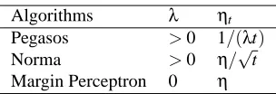
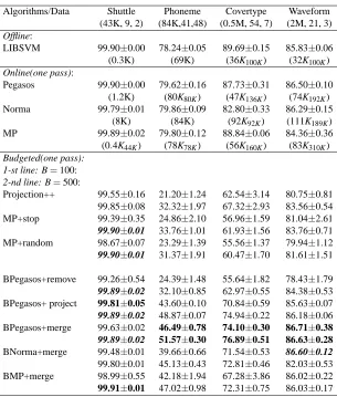
The accuracy of different algorithms on test data is reported in Table 3, 4 and 5.12
Algorithms/Data Banana Gauss Adult IJCNN Checkerb (4.3K, 2, 2) (10K, 2, 2) (21K,123,2) (50K, 21, 2) (10M, 2, 2)
Offline:
LIBSVM Acc: 90.70±0.06 81.62±0.40 84.29±0.0 98.72±0.10 99.87±0.02
(#SVs): (1.1K) (4.0K) (8.5K) (4.9K) (2.6K100K)
Online(one pass):
IDSVM 90.65±0.04 81.67±0.40 83.93±0.03 98.51±0.03 99.40±0.02 (1.1K) (4.0K) (4.0K8.3K) (3.6K33K) (7.5K51K) Pegasos 90.48±0.78 81.54±0.25 84.02±0.14 98.76±0.09 99.35±0.04
(1.7K) (6.4K) (9K) (16K) (41K916K) Norma 90.23±1.04 81.54±0.06 83.65±0.11 93.41±0.15 99.32±0.09
(2.1K) (5.2K) (10K) (33K) (128K730K) MP 89.40±0.57 78.45±2.18 82.61±0.61 98.61±0.10 99.43±0.11
(1K) (3.4K) (8K) (11K) (22K1M)
Budgeted(one pass): 1-st line: B=100:
2-nd line: B=500:
TVM 90.03±0.96 81.56±0.16 82.77±0.00 97.20±0.19 98.90±0.09
91.13±0.68 81.39±0.50 83.82±0.04 98.32±0.14 99.94±0.03
BPA 90.35±0.37 80.75±0.24 83.38±0.56 93.01±0.53 99.01±0.04
91.30±1.18 81.67±0.42 83.58±0.30 96.20±0.35 99.70±0.01 Projection++ 88.36±1.52 76.06±2.25 77.86±3.45 92.36±1.15 96.92±0.45 86.76±1.27 75.17±4.02 79.80±2.11 94.73±1.95 98.24±0.34 MP+stop 88.07±1.38 74.10±3.00 80.00±1.61 91.13±0.18 86.39±1.12 89.77±0.25 79.68±1.19 81.68±0.90 94.60±0.96 95.43±0.43 MP+random 87.54±1.33 75.68±3.68 79.78±0.88 90.22±1.69 84.24±1.39 88.36±0.99 77.26±1.16 80.40±1.03 91.86±1.39 93.12±0.56
BPegasos+remove 85.63±1.25 79.13±1.40 78.84±0.76 90.73±0.31 83.02±2.12 89.92±0.66 80.70±0.61 81.67±0.44 93.30±0.57 91.82±0.22 BPegasos+project 90.21±1.61 81.25±0.34 83.88±0.33 96.48±0.44 97.27±0.72 90.40±0.47 81.33±0.40 83.84±0.07 97.52±0.62 98.08±0.27 BPegasos+merge 90.17±0.61 81.22±0.40 84.55±0.17 97.27±0.72 99.55±0.12
89.46±0.81 81.34±0.38 83.93±0.41 98.08±0.27 99.83±0.08 BNorma+merge 91.53±1.14 81.27±0.37 84.11±0.25 92.69±0.19 99.16±0.23
90.65±1.28 81.37±0.25 83.80±0.21 91.35±0.13 99.72±0.05
BMP+merge 89.37±1.31 79.57±0.90 83.34±0.36 96.67±0.35 98.24±0.13 89.46±0.50 79.38±0.82 82.97±0.26 98.10±0.41 98.79±0.08
Table 3: Comparison of offline, online, and budgeted online algorithms on 5 benchmark binary classification data sets. Online algorithms (IDSVM, Pegasos, Norma and MP) were early stopped after 10,000 seconds and the number of examples being learned at the time of the early stopping was recorded and shown in the subscript within the #SV parenthesis. LIBSVM was trained on a subset of 100K examples on Checkerboard, Covertype and Waveform due to computational issues. Among the budgeted online algorithms, for each combination of data set and budget, the best accuracy is in bold, while the accuracies that were not significantly worse ( with p>0.05 using the one-sided t-test) are in bold and italic.
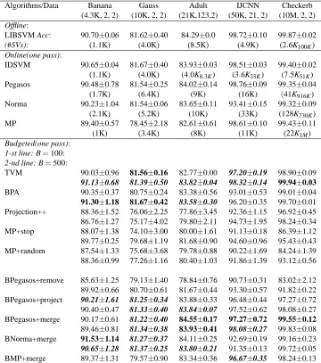
7.5 Comparison of Non-budgeted Algorithms
Algorithms/Data DNA Satimage USPS Pen Letter (4.3K,180, 3) (4.4K, 36, 6) (7.3K,256,10) (7.5K,16, 10) (16K, 16, 26)
Offline:
LIBSVM 95.32±0.00 91.55±0.00 95.27±0.00 98.23±0.00 97.62±0.00
(1.3K) (2.5K) (1.9K) (0.8K) (8.1K)
Online(one pass):
Pegasos 92.87±0.81 91.29±0.15 94.41±0.11 97.86±0.27 96.28±0.15
(0.7K) (2.9K) (4.9K) (1.4K) (8.2K)
Norma 86.15±0.67 90.28±0.35 93.40±0.33 95.86±0.27 95.21±0.09
(2.0K) (4.4K) (6.6K) (7.0K) (15K)
MP 93.36±0.93 91.23±0.54 94.37±0.04 98.02±0.11 96.41±0.24
(0.8K) (1.6K) (2.2K) (1.9K) (8.2K)
Budgeted(one pass): 1-st line: B=100:
2-nd line: B=500:
Projection++ 82.94±3.73 84.47±1.75 81.40±1.26 93.33±0.96 47.23±0.99 90.11±2.11 88.66±0.66 92.02±0.59 95.78±0.75 75.90±0.76 MP+stop 73.56±7.59 82.34±2.43 79.11±2.15 88.27±1.56 41.89±1.16 91.23±0.78 88.68±0.60 90.78±0.58 97.78±0.20 67.32±1.53 MP+random 73.87±4.93 82.51±1.34 78.06±2.01 87.77±2.96 40.93±2.31 87.84±4.84 87.25±1.07 90.10±0.97 97.20±0.68 68.23±1.14
BPegasos+remove 78.63±2.03 81.09±3.21 80.16±1.15 91.84±1.27 41.50±1.49 91.48±1.65 86.77±1.01 89.44±1.05 97.6±0.21 71.97±1.04 BPegasos+ project 86.53±2.03 87.69±0.62 89.67±0.42 96.19±0.85 74.49±1.89 92.26±1.20 88.86±0.2 92.61±0.32 97.58±0.49 87.85±0.49 BPegasos+merge 93.13±1.49 87.53±0.72 91.76±0.24 97.06±0.19 73.63±1.72
92.42±1.24 89.77±0.14 92.91±0.19 97.63±0.14 89.68±0.61
BNorma+merge 75.72±0.25 85.61±0.54 87.44±0.45 90.82±0.42 61.79±1.58 76.25±3.27 86.33±0.40 89.51±0.24 94.60±0.22 75.84±0.35 BMP+merge 93.76±0.31 88.33±0.90 92.31±0.57 97.35±0.16 74.99±1.08 93.84±0.64 90.41±0.22 93.10±0.36 97.86±0.33 88.22±0.36
Table 4: Comparison of offline, online, and budgeted online algorithms on 5 benchmark multi-class data sets
Pegasos, MP, and Norma. Pegasos and MP achieve similar accuracy on most data sets, while Pegasos signif-icantly outperforms MP on the two noisy data sets Gauss and Waveform. Norma is generally less accurate than Pegasos and MP, and the gap is larger on IJCNN, Checkerboard, DNA, and Covertype. Additionally, Norma generates more SVs than its two siblings.
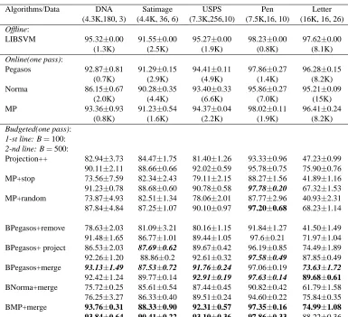
7.6 Comparison of Budgeted Algorithms
Algorithms/Data Shuttle Phoneme Covertype Waveform (43K, 9, 2) (84K,41,48) (0.5M, 54, 7) (2M, 21, 3)
Offline:
LIBSVM 99.90±0.00 78.24±0.05 89.69±0.15 85.83±0.06 (0.3K) (69K) (36K100K) (32K100K)
Online(one pass):
Pegasos 99.90±0.00 79.62±0.16 87.73±0.31 86.50±0.10 (1.2K) (80K80K) (47K136K) (74K192K) Norma 99.79±0.01 79.86±0.09 82.80±0.33 86.29±0.15
(8K) (84K) (92K92K) (111K189K) MP 99.89±0.02 79.80±0.12 88.84±0.06 84.36±0.36
(0.4K44K) (78K78K) (56K160K) (83K310K)
Budgeted(one pass): 1-st line: B=100:
2-nd line: B=500:
Projection++ 99.55±0.16 21.20±1.24 62.54±3.14 80.75±0.81 99.85±0.08 32.32±1.97 67.32±2.93 83.56±0.54 MP+stop 99.39±0.35 24.86±2.10 56.96±1.59 81.04±2.61
99.90±0.01 33.76±1.01 61.93±1.56 83.76±0.71
MP+random 98.67±0.07 23.29±1.39 55.56±1.37 79.94±1.12
99.90±0.01 31.37±1.91 60.47±1.70 81.61±1.51
BPegasos+remove 99.26±0.54 24.39±1.48 55.64±1.82 78.43±1.79
99.89±0.02 32.10±0.85 62.97±0.55 84.38±0.53
BPegasos+ project 99.81±0.05 43.60±0.10 70.84±0.59 85.63±0.07
99.89±0.02 48.87±0.07 74.94±0.22 86.18±0.06
BPegasos+merge 99.63±0.02 46.49±0.78 74.10±0.30 86.71±0.38
99.89±0.02 51.57±0.30 76.89±0.51 86.63±0.28
BNorma+merge 99.48±0.01 39.66±0.66 71.54±0.53 86.60±0.12
99.80±0.01 45.13±0.43 72.81±0.46 82.03±0.53 BMP+merge 98.99±0.55 42.18±1.94 67.28±3.86 86.02±0.22
99.91±0.01 47.02±0.98 72.31±0.75 86.03±0.17
Table 5: Comparison of offline, online, and budgeted online algorithms on 4 benchmark multi-class data sets
7.7 Best Budgeted Algorithm vs Non-budgeted Algorithms
102 103 0.5
0.55 0.6 0.65 0.7 0.75 0.8 0.85 0.9 0.95 1
Budget
accuracy
BPegasos+merge Pegasos
(a)
101 102 103 104
0.7 0.72 0.74 0.76 0.78 0.8 0.82 0.84 0.86 0.88
Budget
accuracy
BPegasos+merge Pegasos
(b) Figure 2: The accuracy of BPegasos as a function of the budget size
−0.5 0 0.5 1 1.5 2 2.5
accuracy improvement
BananaGaussAdultIJCNN
Checkerb DNA
Satimage
USPS PenLetterShuttle
PhonemeCovertypeWaveform
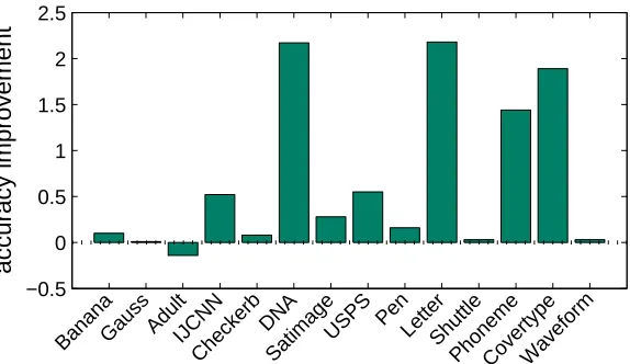
Figure 3: BPegasos+merge (B=500): difference in accuracy between a model trained with 5-passes and a model trained with a single-pass of the data.
7.8 Multi-epoch vs Single-pass Training
For the most accurate budgeted online algorithm BPegasos+merge, we also report its accuracy after allowing it to make 5 passes through training data. In this scenario, BPegasos should be treated as an offline algorithm. The accuracy improvement as compared to the single-pass version is reported in Figure 3. We can observe that multi-epoch training improves the accuracy of BPegasos on most data sets. This result suggests that, if the training time is not of major concern, multiple accesses to the training data should be used.
7.9 Accuracy Evolution Curves
103 104 105 106 107 0.86
0.88 0.9 0.92 0.94 0.96 0.98 1
length of data stream
accuracy
LIBSVM, #SVs=2.6K IDSVM, #SVs=7.5K Pegasos, #SV=41K TVM, B=100, finished in 29Ks BPA, B=100, finished in 4Ks
BPegasos+merge, B=100, finished in 2.5Ks
(a) Checkerboard
102 103 104 105 106
0.74 0.76 0.78 0.8 0.82 0.84 0.86 0.88
length of data stream
accuracy
LIBSVM, #SVs=32K Pegasos, #SVs=90K
BPegasos+merge, B=100, finished in 1.1Ks
(b) Waveform
102 103 104 105
0.5 0.6 0.7 0.8 0.9
length of data stream
accuracy
LIBSVM, #SVs=36K Pegasos, #SVs=90K
BPegasos+merge, B=100, finished in 0.2Ks
(c) Covertype
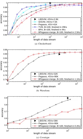
Figure 4: Comparison of accuracy evolution curves
102 103 104 105 106 107 0.8
0.85 0.9 0.95 1
length of data stream
accuracy
BPegasos+merge, B=100, finished in 2.5Ks BPegasos+project, B=100, finished in 1.7Ks BPegasos+remove, B=100, finished in 0.8Ks
(a) Checkerboard
102 103 104 105 106
0.75 0.8 0.85
length of data stream
accuracy
BPegasos+merge, B=100, finished in 1.1Ks BPegasos+project, B=100, finished in 2.4Ks BPegasos+remove, B=100, finished in 0.4Ks
(b) Waveform
102 103 104 105 106
0.5 0.55 0.6 0.65 0.7 0.75
length of data stream
accuracy
BPegasos+merge, B=100, finished in 0.2Ks BPegasos+project, B=100, finished in 0.4Ks BPegasos+remove, B=100, finished in 0.4Ks
(c) Covertype
Figure 5: Accuracy evolution curves of BPegasos for different budget maintenance strategies
104 105 106 107 100
101 102 103 104
length of data stream
training time (seconds)
Pegasos
BPegasos+project, B=100 BPegasos+project, B=500 BPegasos+merge, B=100 BPegasos+merge, B=500
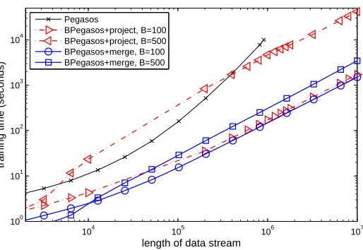
Figure 6: Training time curves on Checkerboard data
Legends in both Figures 4 and 5 list total training time of budgeted algorithms at the end of the data stream (non-budgeted algorithms were early stopped after 10K seconds). Considering that our implementation of all algorithms except LIBSVM was in Matlab and on a 3GB RAM, 3.2GHz Pentium Dual Core 2 PC, Figure 4 indicates a rather impressive speed of the budgeted algorithms. From Figure 5, it can be seen that merging and projection are very fast and are comparable to removal.
7.10 Training Time Scalability
Figure 6 presents log-log plot of the training time versus the data stream length on Checkerboard data set with 10 million examples. Excluding the initial stage, Pegasos had the fastest increase in training time, confirming the expected O(N2)runtime. On the budgeted side, the runtime time of BPegasos with merging and projecting increases linearly with data size. However, it is evident that BPegasos with projecting grow much faster with the budget size than costs of BPegasos with merging. This confirms the expected O(B)
scaling of the merging and O(B2)scaling of the projection version.
7.11 Weight Degradation
Theorems 1, 2, and 3 indicate that lower ¯E leads to lower gap between the optimal solution and the budgeted solution. We also argued that ¯E decreases with budget size through three mechanisms. In Table 6, we show how the value of ¯E on Checkerboard data is being influenced by the budget B and, in turn, how the change in ¯E influences accuracy. From the comparison of three strategies for two B values (100 and 500), we see as B gets larger, ¯E is getting smaller. The results also show that projection and merging achieve significantly lower value than removal and that lower ¯E indeed results in higher accuracy.
7.12 Merged vs Projected SVs
B=100 B=500 ¯
E Acc E¯ Acc
BPegasos+remove 1.402±0.000 79.19±3.05 1.401±0.000 90.32±0.40 BPegasos+project 0.052±0.007 99.25±0.06 0.007±0.001 99.66±0.10 BPegasos+merge 0.037±0.006 99.55±0.14 0.002±0.001 99.74±0.08
Table 6: Comparison of accuracy and averaged weight degradation for three versions of BPegasos as a func-tion of budget size B on 10M Checkerboard examples, using same parameters (λ=10−4, kernel widthσ=0.0625).
(a) BPegasos+project(run 1)
(b) BPegasos+project(run 2)
(c) BPegasos+project(run 3)
(d) BPegasos+merge(run 1)
(e) BPegasos+merge(run 2)
(f) BPegasos+merge(run 3)
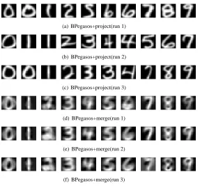
Figure 7: The plot of SVs on USPS data. (Each row corresponds to a different run. 3 different runs using BPegasos+project (B=10) with average accuracy 74%; 3 different runs using BPegasos+merge (B=10) with average accuracy 86%.)
each SV in Figure 7.d-e is blurred and is a result of many mergings of the original labeled examples. This example is a useful illustration of the main difference between projection and merging, and it can be helpful in selecting the appropriate budget maintenance strategy for a particular learning task.
8. Conclusion
number of offline and online, as well as non-budgeted, and budgeted alternatives. The results indicate that highly accurate and compact kernel SVM classifiers can be trained on high-throughput data streams. Partic-ularly, the results show that merging is a highly attractive budget maintenance strategy for BSGD algorithms as it results in relative accurate classifiers while achieving linear training time scaling with support vector budget and data size.
Acknowledgments
This work was supported by the U.S. National Science Foundation Grant IIS-0546155. Koby Crammer is a Horev Fellow, supported by the Taub Foundations.
Appendix A. Proof of Theorem 1
We start by showing the following technical lemma. Lemma 1
• Let Ptbe as defined in (3).
• Let C be a closed convex set with radius U .
• Let w1, ...,wN be a sequence of vectors such that w1∈C and for any t>1 wt+1←∏C(wt−ηt∇t−
∆t),∇t is the (sub)gradient of Pt at wt, ηt is a learning rate function,∆t is a vector, and∏C(w) = arg minw′∈C||w′−w||,is a projection operation that projects w to C.
• Assume||Et|| ≤1.
• Define Dt=||wt−u||2− ||wt+1−u||2as the relative progress toward u at t-th round. Then, the following inequality holds for any u∈C
1 N
N
∑
t=1Pt(wt)− 1 N
N
∑
t=1Pt(u)≤ 1 N
N
∑
t=1Dt 2ηt −
N
∑
t=1λ
2||wt−u||
2+(λU+2)2 2
N
∑
t=1ηt !
+2U ¯E. (20)
Proof of Lemma 1. First, we rewrite wt+1←∏C(wt−ηt∇t−∆t)by treating∆t as the source of error in the gradient wt+1←∏C(wt−ηt∂t),where we defined∂t=∇t+Et.Then, we lower bound Dt as
Dt=||wt−u||2− ||∏C(wt−ηt∂t)−u||2 ≥1||wt−u||2− ||wt−ηt∂t−u||2
=−η2
t||∂t||2+2ηt∇Tt(wt−u) +2ηtEtT(wt−u) ≥2−η2t(λU+1+1)2+2ηt
Pt(wt)−Pt(u) +λ2||wt−u||2
−4ηt||Et||U.
(21)
In≥1, we use the fact that since C is convex,||∏C(a)−b|| ≤ ||a−b||for all b∈C and a. In≥2,||∂t||is bounded as
||∂t|| ≤ ||λwt+ytΦ(xt)||+||Et|| ≤λU+1+1, and, by applying the property of strong convexity, it follows
∇T
t(wt−u)≥Pt(wt)−Pt(u) +λ||wt−u||2/2,