Multiple Kernel Learning Algorithms
Mehmet G¨onen [email protected]
Ethem Alpaydın [email protected]
Department of Computer Engineering Bo˘gazic¸i University
TR-34342 Bebek, ˙Istanbul, Turkey
Editor: Francis Bach
Abstract
In recent years, several methods have been proposed to combine multiple kernels instead of using a single one. These different kernels may correspond to using different notions of similarity or may be using information coming from multiple sources (different representations or different feature subsets). In trying to organize and highlight the similarities and differences between them, we give a taxonomy of and review several multiple kernel learning algorithms. We perform experiments on real data sets for better illustration and comparison of existing algorithms. We see that though there may not be large differences in terms of accuracy, there is difference between them in complexity as given by the number of stored support vectors, the sparsity of the solution as given by the number of used kernels, and training time complexity. We see that overall, using multiple kernels instead of a single one is useful and believe that combining kernels in a nonlinear or data-dependent way seems more promising than linear combination in fusing information provided by simple linear kernels, whereas linear methods are more reasonable when combining complex Gaussian kernels.
Keywords: support vector machines, kernel machines, multiple kernel learning
1. Introduction
The support vector machine (SVM) is a discriminative classifier proposed for binary classifica-tion problems and is based on the theory of structural risk minimizaclassifica-tion (Vapnik, 1998). Given a sample of N independent and identically distributed training instances{(xi,yi)}Ni=1 where xi is the D-dimensional input vector and yi ∈ {−1,+1} is its class label, SVM basically finds the lin-ear discriminant with the maximum margin in the feature space induced by the mapping function
Φ:RD→RS. The resulting discriminant function is
f(x) =hw,Φ(x)i+b.
The classifier can be trained by solving the following quadratic optimization problem:
minimize 1 2kwk
2 2+C
N
∑
i=1 ξi
with respect to w∈RS, ξ∈RN
+, b∈R
subject to yi(hw,Φ(xi)i+b)≥1−ξi ∀i
of the separating hyperplane. Instead of solving this optimization problem directly, the Lagrangian dual function enables us to obtain the following dual formulation:
maximize N
∑
i=1 αi−
1 2
N
∑
i=1
N
∑
j=1
αiαjyiyjhΦ(xi),Φ(xj)i
| {z }
k(xi,xj)
with respect to α∈RN+
subject to N
∑
i=1
αiyi=0
C≥αi≥0 ∀i
where k : RD×RD→Ris named the kernel function and αis the vector of dual variables corre-sponding to each separation constraint. Solving this, we get w=∑Ni=1αiyiΦ(xi)and the discriminant function can be rewritten as
f(x) =
N
∑
i=1
αiyik(xi,x) +b.
There are several kernel functions successfully used in the literature, such as the linear kernel (kLIN), the polynomial kernel (kPOL), and the Gaussian kernel (kGAU):
kLIN(xi,xj) =hxi,xji
kPOL(xi,xj) = (hxi,xji+1)q, q∈N
kGAU(xi,xj) =exp −kxi−xjk22/s2
, s∈R++.
There are also kernel functions proposed for particular applications, such as natural language pro-cessing (Lodhi et al., 2002) and bioinformatics (Sch¨olkopf et al., 2004).
Selecting the kernel function k(·,·)and its parameters (e.g., q or s) is an important issue in train-ing. Generally, a cross-validation procedure is used to choose the best performing kernel function among a set of kernel functions on a separate validation set different from the training set. In recent years, multiple kernel learning (MKL) methods have been proposed, where we use multiple kernels instead of selecting one specific kernel function and its corresponding parameters:
kη(xi,xj) = fη({km(xmi ,xmj)}Pm=1)
where the combination function, fη:RP→R, can be a linear or a nonlinear function. Kernel
func-tions,{km:RDm×RDm →R}Pm=1, take P feature representations (not necessarily different) of data
instances: xi={xmi }Pm=1where xmi ∈RDm, and Dmis the dimensionality of the corresponding feature representation.ηparameterizes the combination function and the more common implementation is
kη(xi,xj) = fη({km(xmi ,xmj)}Pm=1|η)
where the parameters are used to combine a set of predefined kernels (i.e., we know the kernel functions and corresponding kernel parameters before training). It is also possible to view this as
where the parameters integrated into the kernel functions are optimized during training. Most of the existing MKL algorithms fall into the first category and try to combine predefined kernels in an optimal way. We will discuss the algorithms in terms of the first formulation but give the details of the algorithms that use the second formulation where appropriate.
The reasoning is similar to combining different classifiers: Instead of choosing a single kernel function and putting all our eggs in the same basket, it is better to have a set and let an algorithm do the picking or combination. There can be two uses of MKL: (a) Different kernels correspond to different notions of similarity and instead of trying to find which works best, a learning method does the picking for us, or may use a combination of them. Using a specific kernel may be a source of bias, and in allowing a learner to choose among a set of kernels, a better solution can be found. (b) Different kernels may be using inputs coming from different representations possibly from different sources or modalities. Since these are different representations, they have different measures of similarity corresponding to different kernels. In such a case, combining kernels is one possible way to combine multiple information sources. Noble (2004) calls this method of combining kernels
intermediate combination and contrasts this with early combination (where features from different
sources are concatenated and fed to a single learner) and late combination (where different features are fed to different classifiers whose decisions are then combined by a fixed or trained combiner).
There is significant amount of work in the literature for combining multiple kernels. Section 2 identifies the key properties of the existing MKL algorithms in order to construct a taxonomy, highlighting similarities and differences between them. Section 3 categorizes and discusses the existing MKL algorithms with respect to this taxonomy. We give experimental results in Section 4 and conclude in Section 5. The lists of acronyms and notation used in this paper are given in Appendices A and B, respectively.
2. Key Properties of Multiple Kernel Learning
We identify and explain six key properties of the existing MKL algorithms in order to obtain a meaningful categorization. We can think of these six dimensions (though not necessarily orthogo-nal) defining a space in which we can situate the existing MKL algorithms and search for structure (i.e., groups) to better see the similarities and differences between them. These properties are the learning method, the functional form, the target function, the training method, the base learner, and the computational complexity.
2.1 The Learning Method
The existing MKL algorithms use different learning methods for determining the kernel combina-tion funccombina-tion. We basically divide them into five major categories:
1. Fixed rules are functions without any parameters (e.g., summation or multiplication of the kernels) and do not need any training.
3. Optimization approaches also use a parametrized combination function and learn the parame-ters by solving an optimization problem. This optimization can be integrated to a kernel-based learner or formulated as a different mathematical model for obtaining only the combination parameters.
4. Bayesian approaches interpret the kernel combination parameters as random variables, put priors on these parameters, and perform inference for learning them and the base learner parameters.
5. Boosting approaches, inspired from ensemble and boosting methods, iteratively add a new kernel until the performance stops improving.
2.2 The Functional Form
There are different ways in which the combination can be done and each has its own combination parameter characteristics. We group functional forms of the existing MKL algorithms into three basic categories:
1. Linear combination methods are the most popular and have two basic categories: unweighted sum (i.e., using sum or mean of the kernels as the combined kernel) and weighted sum. In the weighted sum case, we can linearly parameterize the combination function:
kη(xi,xj) =fη({km(xmi ,xmj)}Pm=1|η) =
P
∑
m=1
ηmkm(xmi ,xmj)
where ηdenotes the kernel weights. Different versions of this approach differ in the way they put restrictions on η: the linear sum (i.e., η∈RP), the conic sum (i.e., η∈RP+), or
the convex sum (i.e.,η∈RP
+ and∑Pm=1ηm=1). As can be seen, the conic sum is a special case of the linear sum and the convex sum is a special case of the conic sum. The conic and convex sums have two advantages over the linear sum in terms of interpretability. First, when we have positive kernel weights, we can extract the relative importance of the combined kernels by looking at them. Second, when we restrict the kernel weights to be nonnegative, this corresponds to scaling the feature spaces and using the concatenation of them as the combined feature representation:
Φη(x) =
√η
1Φ1(x1) √η
2Φ2(x2)
.. .
√η
PΦP(xP)
and the dot product in the combined feature space gives the combined kernel:
hΦη(xi),Φη(xj)i=
√η
1Φ1(x1i)
√η
2Φ2(x2i) .. .
√η
PΦP(xPi)
⊤
√η
1Φ1(x1j)
√η
2Φ2(x2j) .. .
√η
PΦP(xPj)
= P
∑
m=1
The combination parameters can also be restricted using extra constraints, such as the ℓp -norm on the kernel weights or trace restriction on the combined kernel matrix, in addition to their domain definitions. For example, theℓ1-norm promotes sparsity on the kernel level,
which can be interpreted as feature selection when the kernels use different feature subsets.
2. Nonlinear combination methods use nonlinear functions of kernels, namely, multiplication, power, and exponentiation.
3. Data-dependent combination methods assign specific kernel weights for each data instance. By doing this, they can identify local distributions in the data and learn proper kernel combi-nation rules for each region.
2.3 The Target Function
We can optimize different target functions when selecting the combination function parameters. We group the existing target functions into three basic categories:
1. Similarity-based functions calculate a similarity metric between the combined kernel matrix and an optimum kernel matrix calculated from the training data and select the combination function parameters that maximize the similarity. The similarity between two kernel ma-trices can be calculated using kernel alignment, Euclidean distance, Kullback-Leibler (KL) divergence, or any other similarity measure.
2. Structural risk functions follow the structural risk minimization framework and try to mini-mize the sum of a regularization term that corresponds to the model complexity and an error term that corresponds to the system performance. The restrictions on kernel weights can be integrated into the regularization term. For example, structural risk function can use theℓ1
-norm, theℓ2-norm, or a mixed-norm on the kernel weights or feature spaces to pick the model
parameters.
3. Bayesian functions measure the quality of the resulting kernel function constructed from can-didate kernels using a Bayesian formulation. We generally use the likelihood or the posterior as the target function and find the maximum likelihood estimate or the maximum a posteriori estimate to select the model parameters.
2.4 The Training Method
We can divide the existing MKL algorithms into two main groups in terms of their training method-ology:
1. One-step methods calculate both the combination function parameters and the parameters of the combined base learner in a single pass. One can use a sequential approach or a si-multaneous approach. In the sequential approach, the combination function parameters are determined first, and then a kernel-based learner is trained using the combined kernel. In the simultaneous approach, both set of parameters are learned together.
2.5 The Base Learner
There are many kernel-based learning algorithms proposed in the literature and all of them can be transformed into an MKL algorithm, in one way or another.
The most commonly used base learners are SVM and support vector regression (SVR), due to their empirical success, their ease of applicability as a building block in two-step methods, and their ease of transformation to other optimization problems as a one-step training method using the simultaneous approach. Kernel Fisher discriminant analysis (KFDA), regularized kernel discrimi-nant analysis (RKDA), and kernel ridge regression (KRR) are three other popular methods used in MKL.
Multinomial probit and Gaussian process (GP) are generally used in Bayesian approaches. New inference algorithms are developed for modified probabilistic models in order to learn both the combination function parameters and the base learner parameters.
2.6 The Computational Complexity
The computational complexity of an MKL algorithm mainly depends on its training method (i.e., whether it is one-step or two-step) and the computational complexity of its base learner.
One-step methods using fixed rules and heuristics generally do not spend much time to find the combination function parameters, and the overall complexity is determined by the complexity of the base learner to a large extent. One-step methods that use optimization approaches to learn combina-tion parameters have high computacombina-tional complexity, due to the fact that they are generally modeled as a semidefinite programming (SDP) problem, a quadratically constrained quadratic programming (QCQP) problem, or a second-order cone programming (SOCP) problem. These problems are much harder to solve than a quadratic programming (QP) problem used in the case of the canonical SVM.
Two-step methods update the combination function parameters and the base learner parameters in an alternating manner. The combination function parameters are generally updated by solving an optimization problem or using a closed-form update rule. Updating the base learner parameters usually requires training a kernel-based learner using the combined kernel. For example, they can be modeled as a semi-infinite linear programming (SILP) problem, which uses a generic linear programming (LP) solver and a canonical SVM solver in the inner loop.
3. Multiple Kernel Learning Algorithms
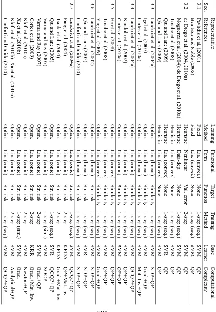
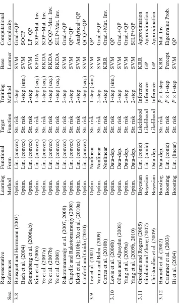
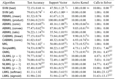
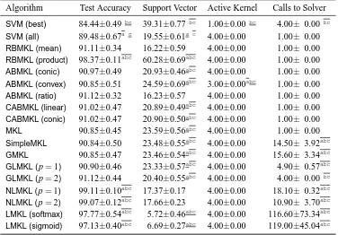
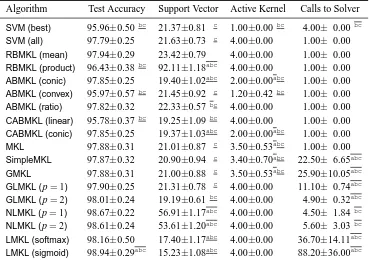
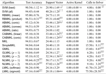
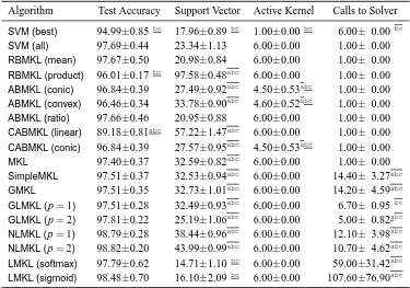
In this section, we categorize the existing MKL algorithms in the literature into 12 groups de-pending on the six key properties discussed in Section 2. We first give a summarizing table (see Tables 1 and 2) containing 49 representative references and then give a more detailed discussion of each group in a separate section reviewing a total of 96 references.
3.1 Fixed Rules
or multiplication of two valid kernels (Cristianini and Shawe-Taylor, 2000):
kη(xi,xj) =k1(x1i,x1j) +k2(x2i,x2j)
kη(xi,xj) =k1(x1i,x1j)k2(x2i,x2j). (1)
We know that a matrix K is positive semidefinite if and only ifυ⊤Kυ≥0, for allυ∈RN. Trivially, we can see that k1(x1i,x1j) +k2(x2i,x2j)gives a positive semidefinite kernel matrix:
υ⊤Kηυ=υ⊤(K1+K2)υ=υ⊤K1υ+υ⊤K2υ≥0
and k1(x1i,x1j)k2(x2i,x2j)also gives a positive semidefinite kernel due to the fact that the element-wise product between two positive semidefinite matrices results in another positive semidefinite matrix:
υ⊤Kηυ=υ⊤(K
1⊙K2)υ≥0.
We can apply the rules in (1) recursively to obtain the rules for more than two kernels. For example, the summation or multiplication of P kernels is also a valid kernel:
kη(xi,xj) =
P
∑
m=1
km(xmi ,xmj)
kη(xi,xj) =
P
∏
m=1
km(xmi ,xmj).
Pavlidis et al. (2001) report that on a gene functional classification task, training an SVM with an unweighted sum of heterogeneous kernels gives better results than the combination of multiple SVMs each trained with one of these kernels.
We need to calculate the similarity between pairs of objects such as genes or proteins especially in bioinformatics applications. Pairwise kernels are proposed to express the similarity between pairs in terms of similarities between individual objects. Two pairs are said to be similar when each object in one pair is similar to one object in the other pair. This approach can be encoded as a pairwise kernel using a kernel function between individual objects, called the genomic kernel (Ben-Hur and Noble, 2005), as follows:
kP({xai,xaj},{xbi,xbj}) =k(xai,xb
i)k(xaj,xbj) +k(xia,xbj)k(xaj,xbi).
Ben-Hur and Noble (2005) combine pairwise kernels in two different ways: (a) using an unweighted sum of different pairwise kernels:
kPη({xai,xa
j},{xbi,xbj}) = P
∑
m=1
kPm({xai,xa
j},{xbi,xbj})
and (b) using an unweighted sum of different genomic kernels in the pairwise kernel:
kηP({xai,xaj},{xbi,xbj})
= P
∑
m=1
km(xai,xbi)
! P
∑
m=1
km(xaj,xbj)
!
+ P
∑
m=1
km(xai,xbj)
! P
∑
m=1
km(xaj,xbi)
!
=kη(xai,xb
i)kη(xaj,xbj) +kη(xia,xbj)kη(xaj,xbi).
3.2 Heuristic Approaches
de Diego et al. (2004, 2010a) define a functional form of combining two kernels:
Kη=1
2(K1+K2) +f(K1−K2)
where the term f(K1−K2)represents the difference of information between what K1and K2
pro-vide for classification. They investigate three different functions:
kη(xi,xj) =
1 2(k1(x
1
i,x1j) +k2(x2i,x2j)) +τyiyj|k1(x1i,x1j)−k2(x2i,x2j)|
kη(xi,xj) =
1 2(k1(x
1
i,x1j) +k2(xi2,x2j)) +τyiyj(k1(x1i,x1j)−k2(x2i,x2j))
Kη=1
2(K1+K2) +τ(K1−K2)(K1−K2)
whereτ∈R+is the parameter that represents the weight assigned to the term f(K1−K2)(selected
through cross-validation) and the first two functions do not ensure having positive semidefinite kernel matrices. It is also possible to combine more than two kernel functions by applying these rules recursively.
Moguerza et al. (2004) and de Diego et al. (2010a) propose a matrix functional form of com-bining kernels:
kη(xi,xj) =
P
∑
m=1
ηm(xi,xj)km(xmi ,xmj)
whereηm(·,·)assigns a weight to km(·,·)according to xi and xj. They propose different heuris-tics to estimate the weighing function values using conditional class probabilities, Pr(yi=yj|xi) and Pr(yj =yi|xj), calculated with a nearest-neighbor approach. However, each kernel function corresponds to a different neighborhood andηm(·,·)is calculated on the neighborhood induced by
km(·,·). For an unlabeled data instance x, they take its class label once as+1 and once as−1, calcu-late the discriminant values f(x|y= +1)and f(x|y=−1), and assign it to the class that has more confidence in its decision (i.e., by selecting the class label with greater y f(x|y)value). de Diego et al. (2010b) use this method to fuse information from several feature representations for face veri-fication. Combining kernels in a data-dependent manner outperforms the classical fusion techniques such as feature-level and score-level methods in their experiments.
We can also use a linear combination instead of a data-dependent combination and formulate the combined kernel function as follows:
kη(xi,xj) =
P
∑
m=1
ηmkm(xmi ,xmj)
where we select the kernel weights by looking at the performance values obtained by each kernel separately. For example, Tanabe et al. (2008) propose the following rule in order to choose the kernel weights for classification problems:
ηm=
πm−δ P
∑
h=1
whereπmis the accuracy obtained using only Km, andδis the threshold that should be less than or equal to the minimum of the accuracies obtained from single-kernel learners. Qiu and Lane (2009) propose two simple heuristics to select the kernel weights for regression problems:
ηm=
Rm
P
∑
h=1
Rh
∀m
ηm= P
∑
h=1
Mh−Mm
(P−1) ∑P h=1
Mh
∀m
where Rm is the Pearson correlation coefficient between the true outputs and the predicted labels generated by the regressor using the kernel matrix Km, and Mmis the mean square error generated by the regressor using the kernel matrix Km. These three heuristics find a convex combination of the input kernels as the combined kernel.
Cristianini et al. (2002) define a notion of similarity between two kernels called kernel
align-ment. The empirical alignment of two kernels is calculated as follows:
A(K1,K2) =p hK1,K2iF
hK1,K1iFhK2,K2iF
wherehK1,K2iF=∑iN=1∑Nj=1k1(x1i,x1j)k2(x2i,x2j). This similarity measure can be seen as the cosine of the angle between K1and K2. yy⊤can be defined as ideal kernel for a binary classification task,
and the alignment between a kernel and the ideal kernel becomes
A(K,yy⊤) = p hK,yy⊤iF
hK,KiFhyy⊤,yy⊤iF
= hK,yy⊤iF
NphK,KiF
.
Kernel alignment has one key property due to concentration (i.e., the probability of deviation from the mean decays exponentially), which enables us to keep high alignment on a test set when we optimize it on a training set.
Qiu and Lane (2009) propose the following simple heuristic for classification problems to select the kernel weights using kernel alignment:
ηm=
A(Km,yy⊤) P
∑
h=1
A(Kh,yy⊤)
∀m (2)
3.3 Similarity Optimizing Linear Approaches with Arbitrary Kernel Weights
Lanckriet et al. (2004a) propose to optimize the kernel alignment as follows:
maximize A(Ktraη,yy⊤) with respect to Kη∈SN
subject to tr Kη=1
Kη0
where the trace of the combined kernel matrix is arbitrarily set to 1. This problem can be converted into the following SDP problem using arbitrary kernel weights in the combination:
maximize *
P
∑
m=1
ηmKtram,yy⊤ +
F with respect to η∈RP, A∈SN
subject to tr(A)≤1
A ∑P
m=1 ηmK⊤m P
∑
m=1
ηmKm I
0
P
∑
m=1
ηmKm0.
Igel et al. (2007) propose maximizing the kernel alignment using gradient-based optimization. They calculate the gradients with respect to the kernel parameters as
∂A(Kη,yy⊤)
∂ηm =
∂Kη
∂ηm
,yy⊤
F
hKη,KηiF− hKη,yy⊤iF ∂Kη
∂ηm
,Kη
F
N
q
hKη,Kηi3F
.
In a transcription initiation site detection task for bacterial genes, they obtain better results by opti-mizing the kernel weights of the combined kernel function that is composed of six sequence kernels, using the gradient above.
Cortes et al. (2010a) give a different kernel alignment definition, which they call centered-kernel
alignment. The empirical centered-alignment of two kernels is calculated as follows:
CA(K1,K2) = h
Kc1,Kc2i F p
hKc
1,Kc1iFhKc2,Kc2iF where Kcis the centered version of K and can be calculated as
Kc=K− 1
N11
⊤K− 1
NK11
⊤+ 1
where 1 is the vector of ones with proper dimension. Cortes et al. (2010a) also propose to optimize the centered-kernel alignment as follows:
maximize CA(Kη,yy⊤)
with respect to η∈
M
(3)where
M
={η:kηk2=1}. This optimization problem (3) has an analytical solution:η= M−
1a kM−1ak
2
(4)
where M={hKcm,KchiF}Pm,h=1and a={hKcm,yy⊤iF}Pm=1.
3.4 Similarity Optimizing Linear Approaches with Nonnegative Kernel Weights
Kandola et al. (2002) propose to maximize the alignment between a nonnegative linear combination of kernels and the ideal kernel. The alignment can be calculated as follows:
A(Kη,yy⊤) =
P
∑
m=1
ηmhKm,yy⊤iF
N
s P
∑
m=1
P
∑
h=1
ηmηhhKm,KhiF
.
We should choose the kernel weights that maximize the alignment and this idea can be cast into the following optimization problem:
maximize A(Kη,yy⊤) with respect to η∈RP
+
and this problem is equivalent to
maximize P
∑
m=1
ηmhKm,yy⊤iF
with respect to η∈RP
+
subject to P
∑
m=1
P
∑
h=1
ηmηhhKm,KhiF =c.
Using the Lagrangian function, we can convert it into the following unconstrained optimization problem:
maximize P
∑
m=1
ηmhKm,yy⊤iF−µ P
∑
m=1
P
∑
h=1
ηmηhhKm,KhiF−c !
Kandola et al. (2002) take µ=1 arbitrarily and add a regularization term to the objective func-tion in order to prevent overfitting. The resulting QP is very similar to the hard margin SVM optimization problem and is expected to give sparse kernel combination weights:
maximize P
∑
m=1
ηmhKm,yy⊤iF− P
∑
m=1
P
∑
h=1
ηmηhhKm,KhiF−λ P
∑
m=1 η2
m
with respect to η∈RP+
where we only learn the kernel combination weights.
Lanckriet et al. (2004a) restrict the kernel weights to be nonnegative and their SDP formulation reduces to the following QCQP problem:
maximize P
∑
m=1
ηmhKtram,yy⊤iF with respect to η∈RP
+
subject to P
∑
m=1
P
∑
h=1
ηmηhhKm,KhiF ≤1. (5)
Cortes et al. (2010a) also restrict the kernel weights to be nonnegative by changing the definition of
M
in (3) to{η:kηk2=1, η∈RP+}and obtain the following QP:
minimize v⊤Mv−2v⊤a
with respect to v∈RP+ (6)
where the kernel weights are given byη=v/kvk2.
3.5 Similarity Optimizing Linear Approaches with Kernel Weights on a Simplex
He et al. (2008) choose to optimize the distance between the combined kernel matrix and the ideal kernel, instead of optimizing the kernel alignment measure, using the following optimization prob-lem:
minimize hKη−yy⊤,Kη−yy⊤i2F
with respect to η∈RP
+
subject to P
∑
m=1
ηm=1.
This problem is equivalent to
minimize P
∑
m=1
P
∑
h=1
ηmηhhKm,KhiF−2 P
∑
m=1
ηmhKm,yy⊤iF
with respect to η∈RP
+
subject to P
∑
m=1
Nguyen and Ho (2008) propose another quality measure called feature space-based kernel ma-trix evaluation measure (FSM) defined as
FSM(K,y) = s++s−
km+−m−k2
where{s+,s−}are the standard deviations of the positive and negative classes, and{m+,m−}are
the class centers in the feature space. Tanabe et al. (2008) optimize the kernel weights for the convex combination of kernels by minimizing this measure:
minimize FSM(Kη,y) with respect to η∈RP
+
subject to P
∑
m=1
ηm=1.
This method gives similar performance results when compared to the SMO-like algorithm of Bach et al. (2004) for a protein-protein interaction prediction problem using much less time and memory. Ying et al. (2009) follow an information-theoretic approach based on the KL divergence be-tween the combined kernel matrix and the optimal kernel matrix:
minimize KL(
N
(0,Kη)kN
(0,yy⊤)) with respect to η∈RP+
subject to P
∑
m=1 ηm=1
where 0 is the vector of zeros with proper dimension. The kernel combinations weights can be optimized using a projected gradient-descent method.
3.6 Structural Risk Optimizing Linear Approaches with Arbitrary Kernel Weights
Lanckriet et al. (2002) follow a direct approach in order to optimize the unrestricted kernel com-bination weights. The implausibility of a kernel matrix,ω(K), is defined as the objective function value obtained after solving a canonical SVM optimization problem (Here we only consider the soft margin formulation, which uses theℓ1-norm on slack variables):
maximize ω(K) = N
∑
i=1 αi−
1 2
N
∑
i=1
N
∑
j=1
αiαjyiyjk(xi,xj)
with respect to α∈RN
+
subject to N
∑
i=1
αiyi=0
C≥αi≥0 ∀i.
The combined kernel matrix is selected from the following set:
K
L= (K : K= P
∑
m=1
where the selected kernel matrix is forced to be positive semidefinite.
The resulting optimization problem that minimizes the implausibility of the combined kernel matrix (the objective function value of the corresponding soft margin SVM optimization problem) is formulated as
minimize ω(Ktraη) with respect to Kη∈
K
Lsubject to tr Kη=c
where Ktraη is the kernel matrix calculated only over the training set and this problem can be cast into the following SDP formulation:
minimize t
with respect to η∈RP, t∈R, λ∈R, ν∈RN
+, δ∈RN+
subject to tr Kη=c
(yy⊤)⊙Ktraη 1+ν−δ+λy
(1+ν−δ+λy)⊤ t−2Cδ⊤1
!
0
Kη0.
This optimization problem is defined for a transductive learning setting and we need to be able to calculate the kernel function values for the test instances as well as the training instances.
Lanckriet et al. (2004a,c) consider predicting function classifications associated with yeast pro-teins. Different kernels calculated on heterogeneous genomic data, namely, amino acid sequences, protein-protein interactions, genetic interactions, protein complex data, and expression data, are combined using an SDP formulation. This gives better results than SVMs trained with each kernel in nine out of 13 experiments. Qiu and Lane (2005) extendsε-tube SVR to a QCQP formulation for regression problems. Conforti and Guido (2010) propose another SDP formulation that removes trace restriction on the combined kernel matrix and introduces constraints over the kernel weights for an inductive setting.
3.7 Structural Risk Optimizing Linear Approaches with Nonnegative Kernel Weights
Lanckriet et al. (2004a) restrict the combination weights to have nonnegative values by selecting the combined kernel matrix from
K
P= (K : K= P
∑
m=1
and reduce the SDP formulation to the following QCQP problem by selecting the combined kernel matrix from
K
Pinstead ofK
L:minimize 1 2ct−
N
∑
i=1 αi
with respect to α∈RN
+, t∈R
subject to tr(Km)t≥α⊤((yy⊤)⊙Ktram)α ∀m N
∑
i=1
αiyi=0
C≥αi≥0 ∀i
where we can jointly find the support vector coefficients and the kernel combination weights. This optimization problem is also developed for a transductive setting, but we can simply take the number of test instances as zero and find the kernel combination weights for an inductive setting. The interior-point methods used to solve this QCQP formulation also return the optimal values of the dual variables that correspond to the optimal kernel weights. Qiu and Lane (2005) give also a QCQP formulation of regression usingε-tube SVR. The QCQP formulation is used for predicting siRNA efficacy by combining kernels over heterogeneous data sources (Qiu and Lane, 2009). Zhao et al. (2009) develop a multiple kernel learning method for clustering problems using the maximum margin clustering idea of Xu et al. (2005) and a nonnegative linear combination of kernels.
Lanckriet et al. (2004a) combine two different kernels obtained from heterogeneous informa-tion sources, namely, bag-of-words and graphical representainforma-tions, on the Reuters-21578 data set. Combining these two kernels with positive weights outperforms the single-kernel results obtained with SVM on four tasks out of five. Lanckriet et al. (2004b) use a QCQP formulation to integrate multiple kernel functions calculated on heterogeneous views of the genome data obtained through different experimental procedures. These views include amino acid sequences, hydropathy profiles, gene expression data and known protein-protein interactions. The prediction task is to recognize the particular classes of proteins, namely, membrane proteins and ribosomal proteins. The QCQP ap-proach gives significantly better results than any single kernel and the unweighted sum of kernels. The assigned kernel weights also enable us to extract the relative importance of the data sources feeding the separate kernels. This approach assigns near zero weights to random kernels added to the candidate set of kernels before training. Dehak et al. (2008) combine three different ker-nels obtained on the same features and get better results than score fusion for speaker verification problem.
A similar result about unweighted and weighted linear kernel combinations is also obtained by Lewis et al. (2006a). They compare the performances of unweighted and weighted sums of kernels on a gene functional classification task. Their results can be summarized with two guidelines: (a) When all kernels or data sources are informative, we should use the unweighted sum rule. (b) When some of the kernels or the data sources are noisy or irrelevant, we should optimize the kernel weights.
task, this method obtains similar results using much less computation time compared to selecting a kernel for standard kernel Fisher discriminant analysis.
Tsuda et al. (2004) learn the kernel combination weights by minimizing an approximation of the cross-validation error for kernel Fisher discriminant analysis. In order to update the kernel com-bination weights, cross-validation error should be approximated with a differentiable error function. They use the sigmoid function for error approximation and derive the update rules of the kernel weights. This procedure requires inverting a N×N matrix and calculating the gradients at each
step. They combine heterogeneous data sources using kernels, which are mixed linearly and non-linearly, for bacteria classification and gene function prediction tasks. Fisher discriminant analysis with the combined kernel matrix that is optimized using the cross-validation error approximation, gives significantly better results than single kernels for both tasks.
In order to consider the capacity of the resulting classifier, Tan and Wang (2004) optimize the nonnegative combination coefficients using the minimal upper bound of the Vapnik-Chervonenkis dimension as the target function.
Varma and Ray (2007) propose a formulation for combining kernels using a linear combination with regularized nonnegative weights. The regularization on the kernel combination weights is achieved by adding a term to the objective function and integrating a set of constraints. The primal optimization problem with these two modifications can be given as
minimize 1 2kwηk
2 2+C
N
∑
i=1 ξi+
P
∑
m=1 σmηm
with respect to wη∈RSη, ξ∈RN
+, b∈R, η∈RP+
subject to yi(hwη,Φη(xi)i+b)≥1−ξi ∀i
Aη≥p
whereΦη(·)corresponds to the feature space that implicitly constructs the combined kernel func-tion kη(xi,xj) =∑Pm=1ηmkm(xmi ,xmj)and wηis the vector of weight coefficients assigned toΦη(·). The parameters A∈RR×P, p∈RR, and σ∈RP encode our prior information about the kernel
weights. For example, assigning higherσivalues to some of the kernels effectively eliminates them by assigning zero weights to them. The corresponding dual formulation is derived as the following SOCP problem:
maximize N
∑
i=1
αi−p⊤δ
with respect to α∈RN+, δ∈RP+
subject to σm−δ⊤A(:,k)≥ 1 2
N
∑
i=1
N
∑
j=1
αiαjyiyjkm(xmi ,xmj) ∀m
N
∑
i=1
αiyi=0 ∀m
C≥αi≥0 ∀i.
problem to find the support vector coefficients at each iteration. The primal optimization problem for givenηis written as
minimize J(η) =1 2kwηk
2 2+C
N
∑
i=1 ξi+
P
∑
m=1 σmηm
with respect to wη∈RSη, ξ∈RN+, b∈R
subject to yi(hwη,Φη(xi)i+b)≥1−ξi ∀i
and the corresponding dual optimization problem is
maximize J(η) = N
∑
i=1 αi−
1 2
N
∑
i=1
N
∑
j=1
αiαjyiyj P
∑
m=1
ηmkm(xmi ,xmj) !
| {z }
kη(xi,xj)
+ P
∑
m=1 σmηm
with respect to α∈RN
+
subject to N
∑
i=1
αiyi=0 ∀m
C≥αi≥0 ∀i.
The gradients with respect to the kernel weights are calculated as
∂J(η)
∂ηm
=σm− 1 2
N
∑
i=1
N
∑
j=1
αiαjyiyj
∂kη(xi,xj)
∂ηm
=σm− 1 2
N
∑
i=1
N
∑
j=1
αiαjyiyjkm(xmi ,xmj) ∀m
and these gradients are used to update the kernel weights while considering nonnegativity and other constraints.
Usually, the kernel weights are constrained by a trace or the ℓ1-norm regularization. Cortes et al. (2009) discuss the suitability of the ℓ2-norm for MKL. They combine kernels with ridge regression using theℓ2-norm regularization over the kernel weights. They conclude that using the ℓ1-norm improves the performance for a small number of kernels, but degrades the performance when combining a large number of kernels. However, theℓ2-norm never decreases the performance and increases it significantly for larger sets of candidate kernels. Yan et al. (2009) compare the
ℓ1-norm and theℓ2-norm for image and video classification tasks, and conclude that theℓ2-norm
should be used when the combined kernels carry complementary information.
constraining them (kηkpp≤1). The resulting optimization problem is
maximize N
∑
i=1 αi−
1 2
P
∑
m=1
N
∑
i=1
N
∑
j=1
αiαjyiyjkm(xmi ,xmj) !p−1
p
p
p−1
with respect to α∈RN
+
subject to N
∑
i=1
αiyi=0
C≥αi≥0 ∀i
and they solve this problem using alternative optimization strategies based on Newton-descent and cutting planes. Xu et al. (2010b) add an entropy regularization term instead of constraining the norm of the kernel weights and derive an efficient and smooth optimization framework based on Nesterov’s method.
Kloft et al. (2010b) and Xu et al. (2010a) propose an efficient optimization method for arbitrary
ℓp-norms with p≥1. Although they approach the problem from different perspectives, they find the same closed-form solution for updating the kernel weights at each iteration. Kloft et al. (2010b) use a block coordinate-descent method and Xu et al. (2010a) use the equivalence between group Lasso and MKL, as shown by Bach (2008) to derive the update equation. Both studies formulate an alternating optimization method that solves an SVM at each iteration and update the kernel weights as follows:
ηm= k
wmk
2 p+1 2
P
∑
h=1k whk
2p p+1 2
1 p
(8)
wherekwmk22=ηm2∑Ni=1∑Nj=1αiαjyiyjkm(xmi ,xmj)from the duality conditions.
When we restrict the kernel weights to be nonnegative, the SDP formulation of Conforti and Guido (2010) reduces to a QCQP problem.
Lin et al. (2009) propose a dimensionality reduction method that uses multiple kernels to embed data instances from different feature spaces to a unified feature space. The method is derived from a graph embedding framework using kernel matrices instead of data matrices. The learning phase is performed using a two-step alternate optimization procedure that updates the dimensionality re-duction coefficients and the kernel weights in turn. McFee and Lanckriet (2009) propose a method for learning a unified space from multiple kernels calculated over heterogeneous data sources. This method uses a partial order over pairwise distances as the input and produces an embedding us-ing graph-theoretic tools. The kernel (data source) combination rule is learned by solvus-ing an SDP problem and all input instances are mapped to the constructed common embedding space.
Another possibility is to allow only binaryηmfor kernel selection. We get rid of kernels whose
The defined kernel function can be expressed as
kη(xi,xj) =
D
∑
m=1
ηmk(xi[m],xj[m])
where[·]indexes the elements of a vector andη∈ {0,1}D. For efficient learning,ηis relaxed into the continuous domain (i.e., 1≥η≥0). Following Lanckriet et al. (2004a), an SDP formulation is derived and this formulation is cast into a QCQP problem to reduce the time complexity.
3.8 Structural Risk Optimizing Linear Approaches with Kernel Weights on a Simplex
We can think of kernel combination as a weighted average of kernels and consider η∈RP + and ∑P
m=1ηm=1. Joachims et al. (2001) show that combining two kernels is beneficial if both of them achieve approximately the same performance and use different data instances as support vectors. This makes sense because in combination, we want kernels to be useful by themselves and com-plementary. In a web page classification experiment, they show that combining the word and the hyperlink representations through the convex combination of two kernels (i.e., η2 =1−η1) can
achieve better classification accuracy than each of the kernels.
Chapelle et al. (2002) calculate the derivative of the margin and the derivative of the radius (of the smallest sphere enclosing the training points) with respect to a kernel parameter,θ:
∂kwk22 ∂θ =−
N
∑
i=1
N
∑
j=1
αiαjyiyj
∂k(xi,xj)
∂θ ∂R2
∂θ =
N
∑
i=1 βi
∂k(xi,xi)
∂θ −
N
∑
i=1
N
∑
j=1 βiβj
∂k(xi,xj)
∂θ
where α is obtained by solving the canonical SVM optimization problem and β is obtained by solving the QP problem defined by Vapnik (1998). These derivatives can be used to optimize the individual parameters (e.g., scaling coefficient) on each feature using an alternating optimization procedure (Weston et al., 2001; Chapelle et al., 2002; Grandvalet and Canu, 2003). This strategy is also a multiple kernel learning approach, because the optimized parameters can be interpreted as the kernel parameters and we combine these kernel values over all features.
Bousquet and Herrmann (2003) rewrite the gradient of the margin by replacing K with Kηand taking the derivative with respect to the kernel weights gives
∂kwηk22 ∂ηm
=− N
∑
i=1
N
∑
j=1
αiαjyiyj
∂kη(xi,xj)
∂ηm
=− N
∑
i=1
N
∑
j=1
αiαjyiyjkm(xmi ,xmj) ∀m
where wηis the weight vector obtained using Kη in training. In an iterative manner, an SVM is trained to obtainα, thenηis updated using the calculated gradient while considering nonnegativity (i.e.,η∈RP
Bach et al. (2004) propose a modified primal formulation that uses the weighted ℓ1-norm on
feature spaces and theℓ2-norm within each feature space. The modified primal formulation is
minimize 1 2
P
∑
m=1
dmkwmk2
!2
+C
N
∑
i=1 ξi
with respect to wm∈RSm, ξ∈RN+, b∈R
subject to yi P
∑
m=1
hwm,Φm(xmi )i+b !
≥1−ξi ∀i
where the feature space constructed using Φm(·) has the dimensionality Sm and the weight dm. When we consider this optimization problem as an SOCP problem, we obtain the following dual formulation:
minimize 1 2γ
2 −
N
∑
i=1 αi
with respect to γ∈R, α∈RN+
subject to γ2dm2 ≥
N
∑
i=1
N
∑
j=1
αiαjyiyjkm(xmi ,xmj) ∀m
N
∑
i=1
αiyi=0
C≥αi≥0 ∀i (9)
where we again get the optimal kernel weights from the optimal dual variables and the weights satisfy∑Pm=1dm2ηm=1. The dual problem is exactly equivalent to the QCQP formulation of Lanck-riet et al. (2004a) when we take dm=
p
tr(Km)/c. The advantage of the SOCP formulation is
that Bach et al. (2004) devise an SMO-like algorithm by adding a Moreau-Yosida regularization term, 1/2∑Pm=1a2mkwmk22, to the primal objective function and deriving the corresponding dual
for-mulation. Using theℓ1-norm on feature spaces, Yamanishi et al. (2007) combine tree kernels for identifying human glycans into four blood components: leukemia cells, erythrocytes, plasma, and serum. Except on plasma task, representing glycans as rooted trees and combining kernels improve performance in terms of the area under the ROC curve. ¨Ozen et al. (2009) use the formulation of Bach et al. (2004) to combine different feature subsets for protein stability prediction problem and extract information about the importance of these subsets by looking at the learned kernel weights.
Sonnenburg et al. (2006a,b) rewrite the QCQP formulation of Bach et al. (2004):
minimize γ
with respect to γ∈R, α∈RN
+
subject to N
∑
i=1
αiyi=0
C≥αi≥0 ∀i
γ≥12
N
∑
i=1
N
∑
j=1
αiαjyiyjkm(xmi ,xmj)− N
∑
i=1 αi
| {z }
Sm(α)
∀m
and convert this problem into the following SILP problem:
maximize θ
with respect to θ∈R, η∈RP
+
subject to P
∑
m=1 ηm=1
P
∑
m=1
ηmSm(α)≥θ ∀α∈ {α:α∈RN, α⊤y=0, C≥α≥0}
where the problem has infinitely many constraints due to the possible values ofα.
The SILP formulation has lower computational complexity compared to the SDP and QCQP formulations. Sonnenburg et al. (2006a,b) use a column generation approach to solve the resulting SILPs using a generic LP solver and a canonical SVM solver in the inner loop. Both the LP solver and the SVM solver can use the previous optimal values for hot-start to obtain the new optimal values faster. These allow us to use the SILP formulation to learn the kernel combination weights for hundreds of kernels on hundreds of thousands of training instances efficiently. For example, they perform training on a real-world splice data set with millions of instances from computational biology with string kernels. They also generalize the idea to regression, one-class classification, and strictly convex and differentiable loss functions.
Kim et al. (2006) show that selecting the optimal kernel from the set of convex combinations over the candidate kernels can be formulated as a convex optimization problem. This formulation is more efficient than the iterative approach of Fung et al. (2004). Ye et al. (2007a) formulate an SDP problem inspired by Kim et al. (2006) for learning an optimal kernel over a convex set of candidate kernels for RKDA. The SDP formulation can be modified so that it can jointly optimize the kernel weights and the regularization parameter. Ye et al. (2007b, 2008) derive QCQP and SILP formulations equivalent to the previous SDP problem in order to reduce the time complexity. These three formulations are directly applicable to multiclass classification because it uses RKDA as the base learner.
each kernel in the set of candidate kernels is used in the combined kernel and we obtain a more regularized solution.
Zien and Ong (2007) develop a QCQP formulation and convert this formulation in two differ-ent SILP problems for multiclass classification. They show that their formulation is the multiclass generalization of the previously developed binary classification methods of Bach et al. (2004) and Sonnenburg et al. (2006b). The proposed multiclass formulation is tested on different bioinfor-matics applications such as bacterial protein location prediction (Zien and Ong, 2007) and protein subcellular location prediction (Zien and Ong, 2007, 2008), and outperforms individual kernels and unweighted sum of kernels. Hu et al. (2009) combine the MKL formulation of Zien and Ong (2007) and the sparse kernel learning method of Wu et al. (2006). This hybrid approach learns the optimal kernel weights and also obtains a sparse solution.
Rakotomamonjy et al. (2007, 2008) propose a different primal problem for MKL and use a projected gradient method to solve this optimization problem. The proposed primal formulation is
minimize 1 2
P
∑
m=1
1
ηmk
wmk22+C
N
∑
i=1 ξi
with respect to wm∈RSm, ξ∈R+N, b∈R, η∈RP+
subject to yi P
∑
m=1
hwm,Φm(xmi )i+b !
≥1−ξi ∀i
P
∑
m=1 ηm=1
and they define the optimal SVM objective function value givenηas J(η):
minimize J(η) =1 2
P
∑
m=1
1
ηmk
wmk22+C
N
∑
i=1 ξi
with respect to wm∈RSm, ξ∈RN+, b∈R
subject to yi P
∑
m=1
hwm,Φm(xmi )i+b !
≥1−ξi ∀i.
Due to strong duality, one can also calculate J(η)using the dual formulation:
maximize J(η) = N
∑
i=1 αi−
1 2
N
∑
i=1
N
∑
j=1
αiαjyiyj P
∑
m=1
ηmkm(xmi ,xmj) !
| {z }
kη(xi,xj)
with respect to α∈RN
+
subject to N
∑
i=1
αiyi=0
The primal formulation can be seen as the following constrained optimization problem:
minimize J(η)
with respect to η∈RP
+
subject to P
∑
m=1
ηm=1. (10)
The overall procedure to solve this problem, called SIMPLEMKL, consists of two main steps: (a) solving a canonical SVM optimization problem with givenηand (b) updatingηusing the following gradient calculated withαfound in the first step:
∂J(η)
∂ηm =−1
2 N
∑
i=1
N
∑
j=1
αiαjyiyj
∂kη(xmi ,xm j)
∂ηm
=−1 2
N
∑
i=1
N
∑
j=1
αiαjyiyjkm(xmi ,xmj) ∀m.
The gradient update procedure must consider the nonnegativity and normalization properties of the kernel weights. The derivative with respect to the kernel weights is exactly equivalent (up to a multiplicative constant) to the gradient of the margin calculated by Bousquet and Herrmann (2003). The overall algorithm is very similar to the algorithm used by Sonnenburg et al. (2006a,b) to solve an SILP formulation. Both algorithms use a canonical SVM solver in order to calculate α at each step. The difference is that they use different updating procedures forη, namely, a projected gradient update and solving an LP. Rakotomamonjy et al. (2007, 2008) show that SIMPLEMKL is more stable than solving the SILP formulation. SIMPLEMKL can be generalized to regression, one-class and multiclass classification (Rakotomamonjy et al., 2008).
Chapelle and Rakotomamonjy (2008) propose a second order method, called HESSIANMKL, extending SIMPLEMKL. HESSIANMKL updates kernel weights at each iteration using a con-strained Newton step found by solving a QP problem. Chapelle and Rakotomamonjy (2008) show that HESSIANMKL converges faster than SIMPLEMKL.
Xu et al. (2009a) propose a hybrid method that combines the SILP formulation of Sonnenburg et al. (2006b) and SIMPLEMKL of Rakotomamonjy et al. (2008). The SILP formulation does not regularize the kernel weights obtained from the cutting plane method and SIMPLEMKL uses the gradient calculated only in the last iteration. The proposed model overcomes both disadvantages and finds the kernel weights for the next iteration by solving a small QP problem; this regularizes the solution and uses the past information.
The alternating optimization method proposed by Kloft et al. (2010b) and Xu et al. (2010a) learns a convex combination of kernels when we use theℓ1-norm for regularizing the kernel weights. When we take p=1, the update equation in (8) becomes
ηm= k
wmk2 P
∑
h=1k whk2
. (11)
The SDP formulation of Conforti and Guido (2010) reduces to a QCQP problem when we use a convex combination of the base kernels.
of sparsity of the combined kernels. The extra regularization term is
λ
∑
Pm=1
ηm− 1
P
2
=λ P
∑
m=1 η2
m−
λ
P =
+λ
∑
Pm=1 η2
m
whereλis regularization parameter that determines the solution sparsity. For example, large values ofλforce the mathematical model to use all the kernels with a uniform weight, whereas small values produce sparse combinations.
Micchelli and Pontil (2005) try to learn the optimal kernel over the convex hull of predefined basic kernels by minimizing a regularization functional. Their analysis shows that any optimizing kernel can be expressed as the convex combination of basic kernels. Argyriou et al. (2005, 2006) build practical algorithms for learning a suboptimal kernel when the basic kernels are continuously parameterized by a compact set. This continuous parameterization allows selecting kernels from basically an infinite set, instead of a finite number of basic kernels.
Instead of selecting kernels from a predefined finite set, we can increase the number of candi-date kernels in an iterative manner. We can basically select kernels from an uncountably infinite set constructed by considering base kernels with different kernel parameters ( ¨Oz¨o˘g¨ur-Aky¨uz and Weber, 2008; Gehler and Nowozin, 2008). Gehler and Nowozin (2008) propose a forward selection algorithm that finds the kernel weights for a fixed size of candidate kernels using one of the methods described above, then adds a new kernel to the set of candidate kernels, until convergence.
Most MKL methods do not consider the group structure between the kernels combined. For example, a group of kernels may be calculated on the same set of features and even if we assign a nonzero weight to only one of them, we have to extract the features in the testing phase. When kernels have such a group structure, it is reasonable to pick all or none of them in the combined kernel. Szafranski et al. (2008, 2010) follow this idea and derive an MKL method by changing the mathematical model used by Rakotomamonjy et al. (2007). Saketha Nath et al. (2010) propose an-other MKL method that considers the group structure between the kernels and this method assumes that every kernel group carries important information. The proposed formulation enforces theℓ∞ -norm at the group level and theℓ1-norm within each group. By doing this, each group is used in the
final learner, but sparsity is promoted among kernels in each group. They formulate the problem as an SCOP problem and give a highly efficient optimization algorithm that uses a mirror-descent approach.
Subrahmanya and Shin (2010) generalize group-feature selection to kernel selection by intro-ducing a log-based concave penalty term for obtaining extra sparsity; this is called sparse multiple kernel learning (SMKL). The reason for adding this concave penalty term is explained as the lack of ability of convex MKL methods to obtain sparse formulations. They show that SMKL obtains more sparse solutions than convex formulations for signal processing applications.
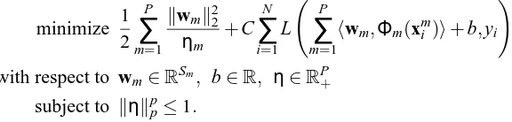
Most of the structural risk optimizing linear approaches can be casted into a general framework (Kloft et al., 2010a,b). The unified optimization problem with the Tikhonov regularization can be written as
minimize 1 2
P
∑
m=1 kwmk22
ηm +C
N
∑
i=1 L
P
∑
m=1
hwm,Φm(xmi )i+b,yi !
+µkηkpp