Hyper-Sparse Optimal Aggregation

(1)

Hyper-Sparse Optimal Aggregation

St´ephane Ga¨ıffas [email protected]

Laboratoire de Statistique Théorique et Appliquée Université Pierre et Marie Curie - Paris 6 75005, Paris, FRANCE

Guillaume Lecu´e [email protected]

CNRS, Laboratoire d’Analyse et Mathématiques appliquées Université Paris-Est - Marne-la-vallée

77454, Marne-la-Valle Cedex 2, FRANCE

Editor: John Shawe-Taylor

Abstract

Given a finite set F of functions and a learning sample, the aim of an aggregation procedure is to have a risk as close as possible to risk of the best function in F. Up to now, optimal aggre-gation procedures are convex combinations of every elements of F. In this paper, we prove that optimal aggregation procedures combining only two functions in F exist. Such algorithms are of particular interest when F contains many irrelevant functions that should not appear in the aggre-gation procedure. Since selectors are suboptimal aggreaggre-gation procedures, this proves that two is the minimal number of elements of F required for the construction of an optimal aggregation pro-cedure in every situations. Then, we perform a numerical study for the problem of selection of the regularization parameters of the Lasso and the Elastic-net estimators. We compare on simulated examples our aggregation algorithms to aggregation with exponential weights, to Mallow’s Cpand to cross-validation selection procedures.

Keywords: aggregation, exact oracle inequality, empirical risk minimization, empirical process

theory, sparsity, Lasso, Lars

1. Introduction

Let(Ω,µ)be a probability space andνbe a probability measure onΩ_×Rsuch that µ is its marginal on Ω. Assume (X,Y) and Dn:= (Xi,Yi)ni=1 to be n+1 independent random variables distributed according toν, and that we are given a finite set F =_{f1, . . . ,fM_}of real-valued functions onΩ, usually called a dictionary, or a set of weak learners. This set of functions is often a set of estimators computed on a training sample, which is independent of the sample Dn(learning sample).

We consider the problem of prediction of Y from X using the functions given in F and the sample Dn. If f :Ω_→R, we measure its error of prediction, or risk, by the expectation of the squared loss

R(f) =E(f(X)₋Y)2. If f depends on Dn, its risk is the conditional expectationb

R(bf) =E[(bf(X)₋Y)2_|_D n].

(2)

satisfies an inequality of the form

R(_f˜₎_≤_min

f∈FR(f) +r(F,n) (1)

with a large probability or in expectation. Inequalities of the form (1) are called exact oracle inequal-ities and r(F,n)is called the residue. A classical result (Juditsky et al., 2008) says that aggregates with values in F cannot satisfy an inequality like (1) with a residue smaller than((log M)/n)1/2_for every F. Nevertheless, it is possible to mimic the oracle (an oracle is a element in F achieving the minimal risk over F) up to the residue(log M)/n (see Juditsky et al., 2008 and Lecu´e and Mendel-son, 2009, among others) using an aggregate ˜f that combines all the elements of F. In this case, we say that ˜f is an optimal aggregation procedure. This notion of optimality is given in Tsybakov (2003) and Lecu´e and Mendelson (2009), and it is the one we will refer to in this paper.

Given the set of functions F, a natural way to predict Y is to compute the empirical risk mini-mization procedure (ERM), the one that minimizes the empirical risk

Rn(f):= 1 n

n

∑

i=1

(Yi−f(Xi))2

over F. This very basic principle is at the core of aggregation procedures (for regression with squared loss). An aggregate is typically represented as a convex combination of the elements of F. Namely,

b

f :=

M

∑

j=1

θj(Dn,F)fj,

where (θj(Dn,F))Mj=1 is a vector of non-negative coordinates suming to 1. Up to now, most of the optimal aggregation procedures are based on exponential weights: aggregation with cumulated exponential weights (ACEW), see Catoni (2001), Yang (2004), Yang (2000), Juditsky et al. (2008), Juditsky et al. (2005), Audibert (2009) and aggregation with exponential weights (AEW), see Leung and Barron (2006) and Dalalyan and Tsybakov (2007), among others. The weights of the ACEW are given by

θ(ACEW)

j := 1 n

n

∑

k=1

exp(₋Rk(fj)/T) ∑M

l=1exp(−Rk(fl)/T) ,

where T is the so-called temperature parameter. The weights of the AEW are given by

θ(AEW)

j :=

exp(₋Rn(fj)/T) ∑M

l=1exp(−Rn(fj)/T) .

The ACEW satisfies (1) for r(F,n)_∼(log M)/n, see references above, so it is optimal in the sense of Tsybakov (2003). The AEW has been proved to be optimal in the regression model with determinis-tic design for large temperatures in Dalalyan and Tsybakov (2007). Altough, for small temperatures, AEW can be suboptimal both in expectation and with large probability (cf. Lecu´e and Mendelson, 2010).

(3)

containing many different types of estimators (kernel estimators, projection estimators, etc.) with many different parameters (smoothing parameters, groups of variables, etc.). Some of the estima-tors are likely to be more adapted than the others, depending on the kind of models that fits well the data, and, there may be only few of them among a large dictionary. An aggregate that combines only the most adapted estimators from the dictionary and that removes the irrelevant ones is suitable in this case. The challenge is then to find such a procedure which is still an optimal aggregate. An improvement going in this direction has been made using a preselection step in Lecu´e and Mendel-son (2009). This preselection step allows to remove all the estimators in F which performs badly on a learning subsample. In this paper, we want to go a step further: we look for an aggregation algorithm that shares the same property of optimality, but with as few non-zero coefficients θj as possible, hence the name hyper-sparse aggregate. This leads to the following question:

Question 1 What is the minimal number of non-zero coefficientsθj such that an aggregation pro-cedure ˜f =∑M

j=1θjfj is optimal?

It turns out that the answer to Question 1 is two. Indeed, if every coefficient is zero, excepted for one, the aggregate coincides with an element of F, and as we mentioned before, such a procedure can only achieve the rate((log M)/n)1/2_{(unless extra properties are satisfied by F and}ν_{). In Definition 1} below (see Section 2) we construct three procedures, where two of them (see (6) and (7)) only have two non-zero coefficientsθj. We prove in Theorem 2 below that these procedures are optimal, since they achieve the rate(log M)/n.

2. Definition of the Aggregates and Results

First, we need to introduce some notations and assumptions. Let us recall that theψ1-norm of a random variable Z is given by _kZ_kψ1 :=inf{c>0 :E[exp(|Z|/c))]≤2}. We say that Z is sub-exponential when_kZ_kψ₁ <+∞. We work under the following assumptions.

Assumption 1 We can write

Y = f0(X) +ε,

where εis such thatE(ε_|X) =0 andE(ε2_|_X₎_≤_σ2

ε a.s. for some constantσε>0. Moreover, we assume that one of the following points holds.

• (Bounded setup) There is a constant b>0 such that:

max_kY_k∞,sup f∈Fk

f(X)_kL∞

≤b. (2)

• (Sub-exponential setup) There is a constant b>0 such that:

max

kεkψ1,sup f∈Fk

f(X)₋f0(X)_kL∞

≤b. (3)

(4)

Definition 1 (Aggregation procedures) Follow the following steps: (0. Initialization) Choose a confidence level x>0. If (2) holds, define

φ=φn,M(x) =b

r

log M+x

n .

If (3) holds, define

φ=φn,M(x) = (σε+b)

r

(log M+x)log n

n .

(1. Splitting) Split the sample D2ninto Dn,1= (Xi,Yi)ni=1and Dn,2= (Xi,Yi)2ni=n+1. (2. Preselection) Use Dn,1to define a random subset of F :

b

F1=nf_∈F : Rn,1(f)≤Rn,1(bfn,1) +c max φkbfn,1−fkn,1,φ2o, (4) where_kf_k2

n,1=n−1∑ni=1f(Xi)2,Rn,1(f) =n−1∑ni=1(f(Xi)−Yi)2, bfn,1∈argminf∈FRn,1(f). (3. Aggregation) Choose

F

b as one of the following sets:

b

F

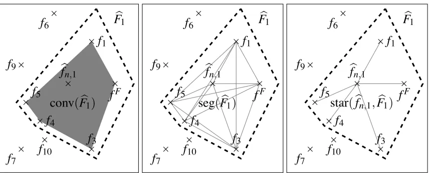
=conv(F1b) = the convex hull ofFb1 (5)

b

F

=seg(Fb1) = the segments between the functions inF1b (6)

b

F

=star(bfn,1,Fb1) = the segments between bfn,1with the elements ofFb1, (7) and return the ERM relative to Dn,2:

˜

f _∈argmin

g∈Fb

Rn,2(g),

where Rn,2(f) =n−1∑2ni=n+1(f(Xi)−Yi)2.

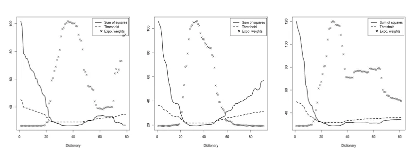
These algorithms are illustrated in Figures 1 and 2. In Figure 1 we summarize the aggregation steps in the three cases. In Figure 2 we give a simulated illustration of the preselection step, and we show the value of the weights of the AEW for a comparison. As mentioned above, the Step 3 of the algorithm returns, when

F

b is given by (6) or (7), an aggregate which is a convex combination of only two functions in F, among the ones remaining after the preselection step. The preselection step was introduced in Lecu´e and Mendelson (2009), with the use of (5) only for the aggregation step.

From the computational point of view, the procedure (7) is the most appealing: an ERM in star(fnb,1,Fb)can be computed in a fast and explicit way, see Algorithm 1 below. The next Theorem proves that each procedure given in Definition 1 are optimal.

Theorem 2 Let x>0 be a confidence level, F be a dictionary with cardinality M and ˜f be one of the aggregation procedure given in Definition 1. If (2) holds, we have, withν2n-probability at least 1₋2e−x:

R(_f˜₎_≤_min

f∈FR(f) +cb

(1+x)log M

(5)

!

F

1

conv

(

F

!

1

)

f

4

f

6

f

1

!

f

n,1

f

3

f

F

f

7

f

5

f

9

f

10

!

F

1

seg

(

F

!

1

)

f

4

f

6

f

1

!

f

n,1

f

3

f

F

f

7

f

5

f

9

f

10

!

F

1

star

(

!

f

n,1

,

F

!

1

)

f

4

f

6

f

1

!

f

n,1

f

3

f

F

f

7

f

5

f

9

f

10

Figure 1: Aggregation algorithms: ERM over conv(F1b),seg(F1b),or star(fnb,1,Fb1).

where cbis a constant depending on b.

If (3) holds, we have, withν2n-probability at least 1₋4e−x: R(f˜)_≤min

f∈FR(f) +cσε,b

(1+x)log M log n

n .

Remark 3 Note that the definition of the setFb1, and thus ˜f , depends on the confidence x through the factorφn,M(x).

Remark 4 To simplify the proofs, we don’t give the explicit values of the constants. However, when (2) holds, one can choose c=4(1+9b)in (4) and c=c1(1+b)when (3) holds (where c1is the absolute constant appearing in Theorem 6). Of course, this is not likely to be the optimal choice.

Now, we give details for the computation of the star-shaped aggregate, namely the aggregate ˜f given by Definition 1 when

F

b is (7). Indeed, ifλ_∈[0,1], we have

Rn,2(λf+ (1−λ)g) =λRn,2(f) + (1−λ)Rn,2(g)−λ(1−λ)kf−gk2n,2, so the minimum ofλ_7→Rn,2(λf+ (1−λ)g)is achieved at

λn,2(f,g) =0∨ 1 2

_R_n_,₂₍_g₎₋_R_n_,₂₍_f₎

kf₋g_k2 n,2

+1_∧1,

where a_∨b=max(a,b), a_∧b=min(a,b). So,

min

λ∈[0,1]Rn,2(λf+ (1−λ)g) =Rn,2(λn,2(f,g)f+ (1−λn,2(f,g))g),

which is equal to

(6)

0 20 40 60 80

40

60

80

100

Dictionary

Sum of squares

Threshold

Expo. weights

0 20 40 60 80

20

40

60

80

100

Dictionary

Sum of squares

Threshold

Expo. weights

0 20 40 60 80

40

60

80

100

120

Dictionary

Sum of squares

Threshold

Expo. weights

Figure 2: Empirical risk Rn,1(f), value of the threshold Rn,1(bfn,1) +2 max(φkbfn,1−fkn,1,φ2)and weights of the AEW (rescaled) for f _∈F, where F is a dictionary obtained using LARS, see Section 3 below. Only the elements of F with an empirical risk smaller than the threshold are kept from the dictionary for the construction of the aggregates of Defi-nition (1). The first and third examples correspond to a case where an aggregate with preselection step improves upon AEW, while in the second example, both procedures behaves similarly.

and to

Rn,2(f) +Rn,2(g)

2 −

(Rn,2(f)−Rn,2(g))2 4_kf₋g_k2_n_,₂ −

kf₋g_k2_n_,₂ 4

if_|Rn,2(f)−Rn,2(g)| ≤ kf−gk2n,2. This leads to the next Algorithm 1 for the computation of ˜f .

3. Simulation Study

(7)

Algorithm 1: Computation of the star-shaped aggregate. Input: dictionary F, data(Xi,Yi)2n

i=1, and a confidence level x>0 Output: star-shaped aggregate ˜f

Split D2ninto two samples Dn,1and Dn,2 foreach j_{∈ {}1, . . . ,M_}do

Compute Rn,1(fj)and Rn,2(fj), and use this loop to find bfn,1∈argminf∈FRn,1(f) end

foreach j∈ {1, . . . ,M}do

Compute_kfj−bfn,1kn,1andkfj−bfn,1kn,2 end

Construct the set of preselected elements

b

F1=

n

f_∈F : Rn,1(f)≤Rn,1(bfn,1) +c max φkbfn,1−fkn,1,φ2

o

,

whereφis given in Definition 1. foreach f _∈Fb1do

compute

Rn,2(λn,2(bfn,1,f)bfn,1+ (1−λn,2(bfn,1,f))f) and keep the element f_b_j_∈Fb1that minimizes this quantity

end return

˜

f=λn,2(bfn,1,f_b_j)bfn,1+ (1−λn,2(bfn,1,f_b_j))f_b_j,

entire sequence of Lasso estimators and a dictionary consisting of entire sequences of the elastic-net estimators (see Zou and Hastie, 2005) corresponding to several ridge penalization parameters, so this dictionary contains the Lasso, the elastic-net, the ridge and the ordinary least-squares estimators.

Remark 5 Note that since an aggregation algorithm is “generic”, in the sense that it can be applied to any dictionary, one could consider larger dictionaries, containing many instances of different type of estimators, for several choices of the tuning parameters, like the Adaptive Lasso (see Zou, 2006) among many other instances of the Lasso. We believe that the conclusion of the numerical study proposed here would be the same as for a much larger dictionary. Indeed, let us recall that here, the focus is on the comparison of selection and aggregation procedures for the choice of tuning parameters, and not on the comparison of the procedures inside the dictionary themselves.

3.1 Examples of Models

We simulate n independent copies of the linear regression model

Y =β⊤X+ε,

(8)

Model 1 (A few effects). We setβ= (3,1.5,0,0,2,0,0,0), so p=8, and we let n to be 20 and 60. The vector X= (X1, . . . ,Xd₎_{is a centered normal vector with covariance matrix Cov}₍_Xi_,Xj_{) =} ρ|i−j|_{, with}_ρ₌_{1/2. The noise}_ε

iis N(0,σ2)withσequal to 1 or 3.

Model 2 (Every effects). This example is the same as Model 1, but withβ= (2,2,2,2,2,2,2,2).

Model 3 (A single effect). This example is the same as Model 1, but withβ= (5,0,0,0,0,0,0,0).

Model 4 (A larger model). We setβ= (010,210_,₀10_,₂10₎_{, where x}y_{stands for the vector of} dimen-sion y with each coordinate equal to x, so p=40. We let n to be 100 and 200. We consider covariates X_ij =Zi,j+Zi where Zi,j and Zi are independent N(0,1)variables. This induces pairwise correlation equal to 0.5 among the covariates. The noiseεiis N(0,σ2)withσequal to 15 or 7.

Model 5 (Sparse vector in high dimension). We set β= (2.55_,1.55_,0.55_,0185₎_{, so p}₌_{200. We} let n to be 50 and 100. The first 15 covariates(X1, . . . ,X15)and the remaining 185 covariates

(X16, . . . ,X200)are independent. Each of these are Gaussian vectors with the same covariance matrix as in Model 1 withρ=0.5. The noise is N(0,σ2₎_with_σ_{equal to 3 and 1.5.}

Model 6 (Sparse vector in high dimension, stronger correlation). This example is the same as Model 5, but withρ=0.95.

3.2 Procedures

We consider a dictionary consisting of the entire sequence of Lasso estimators and a dictionary with several sequences of elastic-net estimators, corresponding to ridge parameters in the set of values {0,0.01,0.1,1,5,10,20,50,100_}(these dictionaries are computed with thelarsandenetroutines fromR).1For each dictionary, we compute the prediction errors_|X(bβ₋β)_|2(where X is the matrix with rows X₁⊤, . . . ,X_n⊤ and _{| · |2} is the ℓn

2-norm of 200 replications (this makes the results stable enough), wherebβis one of the following:

• bβ(Oracle)₌_{the element of the dictionary with smallest prediction error}

• bβ(Cp)₌_{the Lasso estimator selected by Mallows-C}

pheuristic

• bβ(10−Fold)₌_{the element of the dictionary selected by 10-fold cross-validation}

• bβ(Loo)₌_{the element of the dictionary selected by leave-one-out cross-validation}

• bβ(AEW)₌_{The aggregate with exponential weights applied to the dictionary, with temperature}

parameter equal to 4σ2_{, see for instance Dalalyan and Tsybakov (2007)} • bβ(Star)₌_{the star-shaped aggregate applied to the dictionary.}

For the AEW and the star-shaped aggregate, the splits are chosen at random with size[n/2]for training and n₋[n/2]for learning. For both aggregates we use jackknife: we compute the mean of 100 aggregates obtained with several splits chosen at random. This makes the final aggregates less

(9)

dependent on the split. As a matter of fact, we observed in our numerical studies that Star-shaped aggregation with the preselection step and without it (see Definition 1) provides close estimators. So, in order to improve the computational burden, the numerical results of the Star-shaped aggregate reproduced here are the ones obtained without the preselection step.

We need to explain how variable selection is performed based on J star-shaped aggregates com-ing from J random splits (here we take J=100). A Star-shaped aggregate bf(j), corresponding to a split j, can be written as

b

f(j)=bλ(j)_f_b(j)

ERM+ (1−bλ(j))fb

(j)

other,

where bf_ERM(j) is the ERM in F corresponding to the split j and bf_other(j) is the other vertex of the segment where the empirical risk is minimized (recall that the aggregate minimizes the empirical risk over the set of segments star(bf_ERM(j) ,F)). For each split j, we estimate the significance of each covariate using

b

π(j)₌_b_λ(j)₁ b

β(j)

ERM6=0

+ (1₋bλ(j))1_b_β(j)

other6=0 ,

where 1v6=0= (1v16=0, . . . ,1vd6=0). The vectorbπ

(j)_{does a simple average of the contributions of the}

supports of βb(_ERMj) and bβ_other(j) , weighted bybλ(j). To take into consideration each split, we simply compute the mean of the significances of each split:

b

π=1

J J

∑

j=1

b

π(j)_.

The vectorbπcontains the final significances of each covariate. This procedure is close in spirit to the stability selection procedure described in Meinshausen and B¨uhlmann (2010), since each aggregate is related to a subsample. Finally, the selected covariates are the one in

b

S=nk_{∈ {}1, . . . ,p_}:bπk≥bt

o

,

wherebt is a random threshold given by

bt=1

2

1+ bq

2 p2β

,

whereq_b=min(bs,√0.7p),β=p/10 andbs=1_J∑J_j₌₁∑_kp₌₁bπ(kj)is the average sparsity (number of non-zero coefficients) for each splits. This choice of threshold follows the arguments from Meinshausen and B¨uhlmann (2010), together with some empirical tuning.

(10)

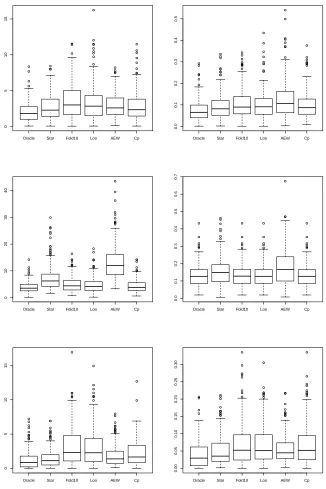
3.3 Conclusion

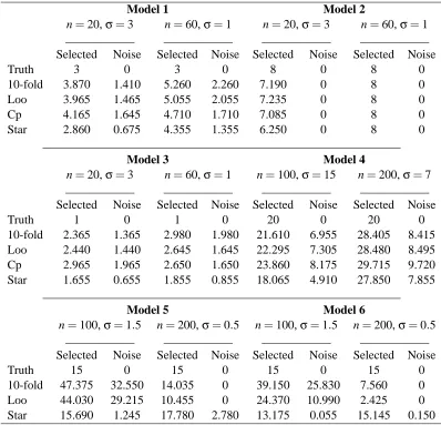
In most cases, the Star-Shaped aggregate improves upon the AEW and the considered selection procedures both in terms of prediction error and variable selection. The proposed variable selection algorithm based on star-shaped aggregation and stability selection tends to select smaller models than the Cp and cross-validation methods (see Table 1, Models 1-4) leading to less noise variables. In particular, in high-dimensional cases (p>n), it is much more stable regarding the sample size and noise level, and provides better results most of the time (see Table 1, Models 5-6). In terms of prediction error, the Star-Shaped always improve the AEW, and is better than the Cp and cross-validations in most cases. We can say that, roughly, the Cp and the cross-validations are better than the Star-Shaped aggregate only for non-sparse vectors (since these selection procedures tend to select larger models), in particular when n is small andσis large. We can conclude by saying that, in the worst cases, the Star-shaped algorithm has prediction and selection performances which are comparable to cross-validations and Cpheuristic, but, on the other hand, it can improve them a lot (in particular for sparse vectors). One can think of the Star-Shaped aggregation algorithm as an alternative to cross-validation and Cp.

Acknowledgments

This work is supported by French Agence Nationale de la Recherce (ANR) ANR Grant “PROG

-NOSTIC” ANR-09-JCJC-0101-01.

Appendix A. Proofs

We will use the following notations. If fF _∈argmin_f_∈_FR(f), we will consider the excess loss

L

_f =

L

_F(f)(X,Y):= (Y₋f(X))2₋₍_Y₋_fF₍_X₎₎2_,

and use the notations

P

L

f :=E

L

f(X,Y), Pn

L

f := 1 n

n

∑

i=1

L

f(Xi,Yi).

A.1 Proof of Theorem 2

Let us prove the result in theψ1case, the other case is similar. Fix x>0 and let

F

b be either (5), (6) or (7). Set d :=diam(Fb1,L2(µ)). Consider the second half of the sample Dn,2= (Xi,Yi)2n_i₌_n₊₁. By Corollary 8 (see Appendix A.2 below), with probability at least 1₋4 exp(₋x)(relative to Dn,2), we have for every f _∈

F

b

1_n

2n

∑

i=1+n

L

_b

F(f)(Xi,Yi)−E

L

Fb(f)(X,Y)|Dn,1

_≤_c₍_σ

ε+b)max(dφ,bφ2),

where

L

_F_b(f)(X,Y):= (f(X)₋Y)2₋₍_fFb₍_X₎

−Y)2_{is the excess loss function relative to}

_F

_b_{, f}Fb

(11)

Oracle Star Fold10 Loo AEW Cp

0

5

10

15

0.0

0.1

0.2

0.3

0.4

0.5

0

10

20

30

40

0.0

0.1

0.2

0.3

0.4

0.5

0.6

0.7

0

5

10

15

0.00

0.05

0.10

0.15

0.20

0.25

0.30

(12)

50

100

150

200

250

300

0

20

40

60

80

Oracle Star Fold10 Loo AEW

5

10

15

0.5

1.0

1.5

2.0

2.5

1

2

3

4

0

1

2

3

4

(13)

Model 1 Model 2

n=20,σ=3 n=60,σ=1 n=20,σ=3 n=60,σ=1

Selected Noise Selected Noise Selected Noise Selected Noise

Truth 3 0 3 0 8 0 8 0

10-fold 3.870 1.410 5.260 2.260 7.190 0 8 0

Loo 3.965 1.465 5.055 2.055 7.235 0 8 0

Cp 4.165 1.645 4.710 1.710 7.085 0 8 0

Star 2.860 0.675 4.355 1.355 6.250 0 8 0

n=20,σ=3 n=60,σ=1 n=100,σ=15 n=200,σ=7

Truth 1 0 1 0 20 0 20 0

10-fold 2.365 1.365 2.980 1.980 21.610 6.955 28.405 8.415

Loo 2.440 1.440 2.645 1.645 22.295 7.305 28.480 8.495

Cp 2.965 1.965 2.650 1.650 23.860 8.175 29.715 9.720

Star 1.655 0.655 1.855 0.855 18.065 4.910 27.850 7.855

n=100,σ=1.5 n=200,σ=0.5 n=100,σ=1.5 n=200,σ=0.5

Truth 15 0 15 0 15 0 15 0

10-fold 47.375 32.550 14.035 0 39.150 25.830 7.560 0

Loo 44.030 29.215 10.455 0 24.370 10.990 2.425 0

Star 15.690 1.245 17.780 2.780 13.175 0.055 15.145 0.150

Table 1: Accuracy of variable prediction in Models 1 to 6 (Lars dictionary)

1 n∑

2n

i=n+1

L

Fb(f˜)(Xi,Yi)≤0, so, on this event (relative to Dn,2)

R(f˜)_≤R(fFb) +E

L

_F_b(f˜)_|Dn,1− 1 n

2n

∑

i=n+1

L

_F_b(f˜)(Xi,Yi)

≤R(fFb) +c(σε+b)max(dφ,bφ2)

=R(fF) +c(σε+b)max(dφ,bφ2)₋ R(fF)₋R(fFb)

=: R(fF) +β,

and it remains to show that

β_≤cb,σε

(1+x)log M log n

n .

(14)

0

2

4

6

8

1

0

1

2

0.0

0.1

0.2

0.3

0.4

0.5

0.6

0.7

0

2

4

6

8

1

0

5

0

1

0

1

5

0

2

0

2

5

0

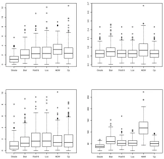
Figure 5: Prediction errors for Models 1 to 4 using the elastic-net dictionary (upper left: Model 1 withσ=3,n=20, upper right: Model 2 withσ=3,n=20, bottom left: Model 3 with σ=3,n=20 and bottom right: Model 4 with n=100,σ=15).

Model 1 Model 2 Model 3 Model 4

n=20,σ=3 n=20,σ=3 n=20,σ=3 n=100,σ=15

Truth 3 0 8 0 1 0 20 0

10-fold 5.040 2.155 7.450 0 3.045 2.045 25.575 9.475

Loo 4.940 2.065 7.460 0 2.980 1.980 25.535 9.660

Cp 4.490 1.660 7.335 0 2.760 1.760 24.345 8.470

Star 4.355 1.475 7.485 0 2.080 1.080 24.090 8.755

(15)

Let us turn out to the situation where

F

b is given by (7). Recall that fnb,1is the ERM onF1b using Dn,1. Consider f1such thatkbfn,1−f1kL2₍_µ₎=max_f

∈Fb1kbfn,1−fkL2(µ), and note that kbfn,1−f1kL2₍_µ₎≤d≤2kbf_n_,₁−f1kL2₍_µ₎.

The mid-point f2:= (bfn,1+ f1)/2 belongs to star(bfn,1,F1b). Using the parallelogram identity, we have for any u,v_∈L2(ν):

Eν

_u₊_v

2

≤Eν(u 2_{) +}_E

ν(v2)

2 −

ku₋v_k2 L2(ν)

4 ,

where for every h∈L2(ν),Eν(h) =Eh(X,Y). In particular, for u(X,Y) = fnb,1−Y and v(X,Y) = f1(X)₋Y , the mid-point is(u(X,Y) +v(X,Y))/2= f2(X)₋Y . Hence,

R(f2) =E(f2(X)₋Y)2=E bfn,1(X) +f1(X)

2 −Y

2

≤1₂E(fbn,1(X)−Y)2+ 1

2E(f1(X)−Y) 2

−1₄kfn,1−f1k2L2(µ) ≤1

2R(bfn,1) + 1

2R(f1)− d2 16,

where the expectations are taken conditioned on Dn,1. By Lemma 10 (see Appendix A.2 below), since bfn,1,f1∈Fb1, we have

1

2R(bfn,1) + 1

2R(f1)≤R(f

F_{) +}_c₍_σ

ε+b)max(φd,bφ2), and thus, since f2∈

F

b

R(fFb)_≤R(f2)_≤R(fF) +c(σε+b)max(φd,bφ2)₋cd2. Therefore,

β=c(σε+b)max(dφ,bφ2)₋ R(fF)₋R(fFb)

≤c(σ_ε+b)max(φd,bφ2₎₋_cd2_.

Finally, if d_≥c_σ_ε,bφthenβ≤0, otherwiseβ≤cσε,bφ2. It concludes the proof of Theorem 2. A.2 Tools from Empirical Process Theory and Technical Results

The following Theorem is a Talagrand’s type concentration inequality (see Talagrand, 1996) for a class of unbounded functions.

Theorem 6 (Theorem 4, Adamczak, 2008) Assume that X,X1, . . . ,Xnare independent random vari-ables and F is a countable set of functions such thatEf(X) =0,_∀f _∈F and_ksup_f_∈_F f(X)_kψ₁ <

+∞. Define

Z :=sup f∈F

1_n

n

∑

(16)

and

σ2₌_sup f_∈FE

f(X)2and b :=_k max

i=1,...,nsup_f_∈_F|f(Xi)|kψ1. Then, for anyη∈(0,1)andδ>0, there is c=c_η,δsuch that for any x>0:

P

h

Z≥(1+η)_EZ+σ r

2(1+δ)x

n+cb

_x

n

i

≤4e−x

PhZ_≤(1₋η)EZ₋σ

r

2(1+δ)x

n−cb

_x

n

i

≤4e−x.

Now we state some technical Lemmas, used in the proof of Theorem 2. Given a sample(Zi)n i=1, we set the random empirical measure Pn:=n−1∑ni=1δZi. For any function f define(P−Pn)(f):=

n−1∑n_i₌₁f(Zi)₋Ef(Z)and for a class of functions F, define_kP₋PnkF :=supf∈F|(P−Pn)(f)|. In all what follows, we denote by c an absolute positive constant, that can vary from place to place. Its dependence on the parameters of the setting is specified in place.

Lemma 7 Define

d(F):=diam(F,L2(µ)), σ2(F) =sup f_∈FE

[f(X)2],

C

=conv(F),

and

L

C(C) ={(Y−f(X))2−(Y−fC(X))2: f ∈

C

}, where fC ∈argmin_g_∈CR(g). If (2) holds, we

have

Ehsup

f∈F 1 n

n

∑

i=1

f2(Xi)i_≤c maxσ2(F),b 2_{log M}

n

,and

EkPn−PkLC(C)≤cb

r log M n max b r log M n ,d(F)

.

If (3) holds, we have

Ehsup

f_∈F 1 n

n

∑

i=1 f2(Xi)

i

≤c maxσ2(F),b 2_{log M}

n

,and

EkPn₋P_kLC(C)≤cb

r

log M log n

n max

b

r

log M log n n ,d(F)

.

Proof First, consider the case (3). Define

r2=sup f∈F 1 n

n

∑

i=1 f(Xi)2,

and note thatEX(r2)≤EXkP−PnkF2+σ(F)2, where F :={f2: f ∈F}. Using the Gin´e-Zinn symmetrization argument, see Gin´e and Zinn (1984), we have

EXkP−PnkF2≤

c nEXEg

h

sup f∈F

n

∑

i=1

(17)

where (gi) are i.i.d. standard normal. The process f 7→Z2,f =∑ni=1gif2(Xi) is Gaussian, with intrinsic distance

Eg|Z2,f−Z2,f′|2= n

∑

i=1

(f(Xi)2₋f′(Xi)2)2_≤dn,∞(f,f′)2×4nr2,

where dn,∞(f,f′) =maxi=1,...,n|f(Xi)−f′(Xi)|. Using (3) we have dn,∞(f,f′)≤2b for any f,f′∈F, so using Dudley’s entropy integral, we have

EgkP₋P_nkF2 ≤

c √ n Z 2b 0 q

log N(F,dn,∞,t)dt≤cr

r

log M n .

So, we get

EXkP−PnkF2 ≤cb

r

log M

n EX[r]≤cb

r

log M n

q

EX[r2], which entails that

EX(r2)≤c max

_b2_{log M}

n +σ(F) 2_.

Let us turn to the part of the Lemma concerningEkP₋PnkLC(C). Recall that

C

=conv(F)and write for short

L

f(X,Y) =

L

C(f)(X,Y) = (Y−f(X))2−(Y−fC(X))2for each f ∈

C

, where we recall

that fC _∈argmin_g_∈CR(g). Using the same argument as before we have

EkP−PnkLC(C)≤

c

nE(X,Y)Eg

h

sup f∈C

n

∑

i=1

gi

L

_f(Xi,Yi)i.

Consider the Gaussian process f _∈

C

_→Zf :=∑ni=1gi

L

f(Xi,Yi)indexed by

C

. For every f,f′∈

C

, the intrinsic distance of(Zf)f∈C satisfies

Eg|Zf−Zf′|2= n

∑

i=1

(Lf(Xi,Yi)−

L

f′(X_i,Y_i))2

≤ max

i=1,...,n|2Yi−f(Xi)−f ′₍_X

i)|2× n

∑

i=1

(f(Xi)−f′(Xi))2

= max

i=1,...,n|2Yi−f(Xi)−f ′₍_X

i)|2×Eg|Z′f−Z′f′|2,

where Z′_f :=∑n_i₌₁gi(f(Xi)₋fC(Xi)). Therefore, by Slepian’s Lemma, we have for every(Xi,Yi)n i=1:

Eg

h

sup f∈C

Zf

i

≤ max

i=1,...,n_fsup_,_f′_∈C|

2Yi−f(Xi)−f′(Xi)| ×Eg

h

sup f∈C

Z′_fi,

and since for every f=∑M_j₌₁αjfj∈

C

, whereαj≥0,∀j=1, . . . ,M and∑αj=1, Z′_f =∑Mj=1αjZfj,

we have

Eg

h

sup f∈C

Z′_f

i

≤Eg

h

sup f∈F

Z′_f

i

.

Moreover, we have, using Dudley’s entropy integral argument,

1 nEg

h

sup f∈F

Z′_f

i

≤√c n

Z _∆_n(F′)

0

p

N(F,_{k · k}n,t)dt_≤c

r

log M n r

(18)

where F′:=_{f−fC : f ∈F}and∆n(F′):=diam(F′,k · kn)and

r′2:=sup f∈F′

1 n

n

∑

i=1 f(Xi)2. Hence, we proved that

EkP₋PnkLC(C)≤c

r

log M n

r

Eh max

i=1,...,n|2Yi−f(Xi)−f

′₍_Xi₎_|2iq_E₍_r′2₎_.

Using Pisier’s inequality forψ1 random variables and the fact thatE(U2)≤4kUkψ1 for any ψ1 -random variable U , together with (3), we obtain that

Eh max

i=1,...,n_f_,sup_f′_∈C|

2Yi−f(Xi)−f′(Xi)|2

i

≤cb2log(n). (8)

So, we finally obtain

EkP₋PnkLC(C)≤c

r

log n log M n

q

E(r′2₎_,

and the conclusion follows from the first part of the Lemma, sinceσ(F′)_≤d(F). The case (2) is easier and follows from the fact that the left hand side of (8) is smaller than 4b.

Lemma 7 combined with Theorem 6 leads to the following corollary.

Corollary 8 Let d(F) =diam(F,L2₍_µ₎₎_,

_C

_:₌_conv₍_F₎_and

_L

f(X,Y) = (Y−f(X))2−(Y−fC(X))2 for any f _∈

C

.

If (3) holds, we have, with probability larger than 1₋4e−x, that for every f _∈

C

:

1_n

n

∑

i=1

L

_f(Xi,Yi)−E

L

f(X,Y)

≤c(σ_ε+b) r

(log M+x)log n

n max

b

r

(log M+x)log n n ,d(F)

.

If (2) holds, we have, with probability larger than 1₋2e−x, that for every f _∈

C

:

1_n

n

∑

i=1

L

f(Xi,Yi)−E

L

f(X,Y)

≤cb

r

log M+x n max

b

r

log M+x n ,d(F)

.

Proof Applying Theorem 6 to

Z :=sup f∈C

1_n

n

∑

i=1

L

_f(Xi,Yi)₋E

L

_f(X,Y),

we obtain that, with a probability larger than 1−4e−x:

Z_≤c

EZ+σ(

C

)

r

x

n+bn(

C

) x n

(19)

where

σ(C)2=sup f∈CE

[Lf(X,Y)2], and bn(C) = max

i=1,...,nsup_f_∈_C|

L

f(Xi,Yi)−E[Lf(X,Y)]|

_ψ

1.

Since

L

f(X,Y) =2ε(fC(X)−f(X)) + (fC(X)−f(X))(2 f0(X)−f(X)−fC(X)), (9)

we have using Assumptions 1 and (3):

E[Lf(X,Y)2]≤(4σ2_ε+2b2)kf−fCk2_L2₍_µ₎, meaning that

σ(C)2_≤(4σ_ε2+2b2)d(F).

SinceE(_|Z_|)_{≤ k}Z_kψ₁, we have bn(C)≤2 log(n+1)ksupf_∈C|

L

f(X,Y)|kψ1. Moreover, using again (9), we obtain that

bn(C)_≤16 log(n+1)b2. Putting all this together, and using Lemma 7, we arrive at

Z_≤c(σε+b) r

(log M+x)log n

n max

b

r

(log M+x)log n n ,d(F)

,

with probability larger than 1₋4e−x for any x>0. In the bounded case (2) the proof is easier, and one can use the original Talagrand’s concentration inequality.

Lemma 9 Let

L

_f(X,Y) = (Y₋f(X))2₋₍_Y₋_fF₍_X₎₎2_{for any f} _∈_F.

If (3) holds, we have with probability larger than 1₋4e−x, that for every f _∈F:

1_n

n

∑

i=1

L

_f(Xi,Yi)−E

L

f(X,Y)

≤c(σε+b) r

(log M+x)log n

n max

b

r

(log M+x)log n n ,kf−f

F k.

Also, with probability at least 1₋4e−x, we have for every f,g_∈F:

_kf₋g_k2_n_{− k}f₋g_k2

≤cb

r

(log M+x)log n

n max

b

r

(log M+x)log n

n ,kf−gk

.

If (2) holds, we have, with probability larger than 1₋2e−x, that for every f _∈F:

1_n

n

∑

i=1

L

_f(Xi,Yi)₋E

L

_f(X,Y)_≤cb

r

log M+x

n max

b

r

log M+x

n ,kf−f F

k,

and with probability at least 1₋2e−x_{, that for every f}_,g_∈_F:

_kf₋g_k2_n_{− k}f₋g_k2_≤cb

r

log M+x

n max

b

r

log M+x

n ,kf−gk

(20)

Proof [Proof of Lemma 9] The proof uses exactly the same arguments as that of Lemma 7 and Corollary 8, and thus is omitted.

Lemma 10 Let Fb1 be given by (4) and recall that fF ∈ argminf∈FR(f) and let d(F1b) = diam(Fb1,L2(µ)).

If (3) holds, we have with probability at least 1₋4 exp(₋x) that fF _∈F1, and any functionb f _∈Fb1satisfies

R(f)_≤R(fF) +c(σε+b) r

(log M+x)log n

n max

b

r

(log M+x)log n n ,d(Fb1)

.

If (2) holds, we have with probability at least 1₋2 exp(₋x) that fF _∈Fb1, and any function f _∈Fb1satisfies

R(f)_≤R(fF) +cb

r

log M+x n max

b

r

log M+x n ,d(F1b)

.

Proof The proof follows the lines of the proof of Lemma 4.4 in Lecu´e and Mendelson (2009), together with Lemma 9, so we don’t reproduce it here.

References

Radosław Adamczak. A tail inequality for suprema of unbounded empirical processes with appli-cations to Markov chains. Electron. J. Probab., 13:no. 34, 1000–1034, 2008. ISSN 1083-6489.

Jean-Yves Audibert. Fast learning rates in statistical inference through aggregation. Ann. Statist.,

37:1591, 2009. URLdoi:10.1214/08-AOS623.

Olivier Catoni. Statistical Learning Theory and Stochastic Optimization. Ecole d’été de Probabilités de Saint-Flour 2001, Lecture Notes in Mathematics. Springer, N.Y., 2001.

Arnak S. Dalalyan and Alexandre B. Tsybakov. Aggregation by exponential weighting and sharp oracle inequalities. In COLT, pages 97–111, 2007.

Bradley Efron, Trevor Hastie, Iain Johnstone, and Robert Tibshirani. Least angle regression. Ann. Statist., 32(2):407–499, 2004. ISSN 0090-5364. With discussion, and a rejoinder by the authors.

Evarist Gin´e and Joel Zinn. Some limit theorems for empirical processes. Ann. Probab., 12(4): 929–998, 1984. ISSN 0091-1798.

Anatoli Juditsky, Alexander V. Nazin, Alexandre B. Tsybakov, and Nicolas Vayatis. Recursive aggregation of estimators by the mirror descent method with averaging. Problemy Peredachi Informatsii, 41(4):78–96, 2005. ISSN 0555-2923.

Anatoli Juditsky, Philippe Rigollet, and Alexandre B. Tsybakov. Learning by mirror averaging. Ann. Statist., 36(5):2183–2206, 2008. ISSN 0090-5364. doi: 10.1214/07-AOS546. URLhttp:

(21)

Guillaume Lecu´e and Shahar Mendelson. Aggregation via empirical risk minimization. Probab. Theory Related Fields, 145(3-4):591–613, 2009. ISSN 0178-8051. doi: 10.1007/

s00440-008-0180-8. URLhttps://dx.doi.org/10.1007/s00440-008-0180-8.

Guillaume Lecu´e and Shahar Mendelson. On the optimality of the aggregate with exponential weights for small temperatures. Submitted, 2010.

Gilbert Leung and Andrew R. Barron. Information theory and mixing least-squares regressions. IEEE Trans. Inform. Theory, 52(8):3396–3410, 2006. ISSN 0018-9448.

Nicolai Meinshausen and Peter B¨uhlmann. Stability selection. Journal of the Royal Statistical Society: Series B (Statistical Methodology), 72(4):417–473, 2010.

Michel Talagrand. New concentration inequalities in product spaces. Invent. Math., 126(3):505– 563, 1996. ISSN 0020-9910.

Robert Tibshirani. Regression shrinkage and selection via the lasso. J. Roy. Statist. Soc. Ser. B, 58 (1):267–288, 1996. ISSN 0035-9246.

Alexandre. B. Tsybakov. Optimal rates of aggregation. Computational Learning Theory and Kernel Machines. B.Sch¨olkopf and M.Warmuth, eds. Lecture Notes in Artificial Intelligence, 2777:303– 313, 2003. Springer, Heidelberg.

Yuhong Yang. Mixing strategies for density estimation. Ann. Statist., 28(1):75–87, 2000.

ISSN 0090-5364. doi: 10.1214/aos/1016120365. URL http://dx.doi.org/10.1214/aos/

1016120365.

Yuhong Yang. Aggregating regression procedures to improve performance. Bernoulli, 10(1):25–47, 2004. ISSN 1350-7265.

Hui Zou. The adaptive lasso and its oracle properties. Journal of the American Statistical Associa-tion, 101(476):1418–1429, 2006.

Hui Zou and Trevor Hastie. Regularization and variable selection via the elastic net. J. R. Stat. Soc. Ser. B Stat. Methodol., 67(2):301–320, 2005. ISSN 1369-7412. doi: 10.1111/j.1467-9868.2005.