Analysis of a Random Forests Model

(1)

Analysis of a Random Forests Model

LSTA & LPMA

Université Pierre et Marie Curie – Paris VI Boˆıte 158, Tour 15-25, 2ème étage

4 place Jussieu, 75252 Paris Cedex 05, France

Editor: Bin Yu

Abstract

Random forests are a scheme proposed by Leo Breiman in the 2000’s for building a predictor ensemble with a set of decision trees that grow in randomly selected subspaces of data. Despite growing interest and practical use, there has been little exploration of the statistical properties of random forests, and little is known about the mathematical forces driving the algorithm. In this paper, we offer an in-depth analysis of a random forests model suggested by Breiman (2004), which is very close to the original algorithm. We show in particular that the procedure is consistent and adapts to sparsity, in the sense that its rate of convergence depends only on the number of strong features and not on how many noise variables are present.

Keywords: random forests, randomization, sparsity, dimension reduction, consistency, rate of convergence

1. Introduction

In a series of papers and technical reports, Breiman (1996, 2000, 2001, 2004) demonstrated that substantial gains in classification and regression accuracy can be achieved by using ensembles of trees, where each tree in the ensemble is grown in accordance with a random parameter. Final predictions are obtained by aggregating over the ensemble. As the base constituents of the ensemble are tree-structured predictors, and since each of these trees is constructed using an injection of randomness, these procedures are called “random forests.”

1.1 Random Forests

Breiman’s ideas were decisively influenced by the early work of Amit and Geman (1997) on geomet-ric feature selection, the random subspace method of Ho (1998) and the random split selection ap-proach of Dietterich (2000). As highlighted by various empirical studies (see for instance Breiman, 2001; Svetnik et al., 2003; Diaz-Uriarte and de Andr´es, 2006; Genuer et al., 2008, 2010), random forests have emerged as serious competitors to state-of-the-art methods such as boosting (Freund and Shapire, 1996) and support vector machines (Shawe-Taylor and Cristianini, 2004). They are fast and easy to implement, produce highly accurate predictions and can handle a very large number of input variables without overfitting. In fact, they are considered to be one of the most accurate general-purpose learning techniques available. The survey by Genuer et al. (2008) may provide the reader with practical guidelines and a good starting point for understanding the method.

(2)

In Breiman’s approach, each tree in the collection is formed by first selecting at random, at each node, a small group of input coordinates (also called features or variables hereafter) to split on and, secondly, by calculating the best split based on these features in the training set. The tree is grown using CART methodology (Breiman et al., 1984) to maximum size, without pruning. This subspace randomization scheme is blended with bagging (Breiman, 1996; B¨uhlmann and Yu, 2002; Buja and Stuetzle, 2006; Biau et al., 2010) to resample, with replacement, the training data set each time a new individual tree is grown.

Although the mechanism appears simple, it involves many different driving forces which make it difficult to analyse. In fact, its mathematical properties remain to date largely unknown and, up to now, most theoretical studies have concentrated on isolated parts or stylized versions of the algo-rithm. Interesting attempts in this direction are by Lin and Jeon (2006), who establish a connection between random forests and adaptive nearest neighbor methods (see also Biau and Devroye, 2010, for further results); Meinshausen (2006), who studies the consistency of random forests in the con-text of conditional quantile prediction; and Biau et al. (2008), who offer consistency theorems for various simplified versions of random forests and other randomized ensemble predictors. Neverthe-less, the statistical mechanism of “true” random forests is not yet fully understood and is still under active investigation.

In the present paper, we go one step further into random forests by working out and solidifying the properties of a model suggested by Breiman (2004). Though this model is still simple compared to the “true” algorithm, it is nevertheless closer to reality than any other scheme we are aware of. The short draft of Breiman (2004) is essentially based on intuition and mathematical heuristics, some of them are questionable and make the document difficult to read and understand. However, the ideas presented by Breiman are worth clarifying and developing, and they will serve as a starting point for our study.

Before we formalize the model, some definitions are in order. Throughout the document, we suppose that we are given a training sample

D

_n={(X1,Y1), . . . ,(Xn,Yn)}of i.i.d.[0,1]d×R-valued

random variables (d≥2) with the same distribution as an independent generic pair(X,Y)satisfying

E_Y2_<∞. The space_[0,1]d _{is equipped with the standard Euclidean metric. For fixed x}_∈_[0,1]d_,

our goal is to estimate the regression function r(x) =E_[_Y_|X₌_x_]_{using the data}

D

n. In this respect,

we say that a regression function estimate rnis consistent ifE[rn(X)−r(X)]2→0 as n→∞. The

main message of this paper is that Breiman’s procedure is consistent and adapts to sparsity, in the sense that its rate of convergence depends only on the number of strong features and not on how many noise variables are present.

1.2 The Model

Formally, a random forest is a predictor consisting of a collection of randomized base regression trees{rn(x,Θm,

D

n),m≥1}, whereΘ1,Θ2, . . .are i.i.d. outputs of a randomizing variableΘ. These

random trees are combined to form the aggregated regression estimate

¯rn(X,

D

n) =EΘ[rn(X,Θ,

D

n)],

whereE_Θ_{denotes expectation with respect to the random parameter, conditionally on X and the data}

set

D

_n. In the following, to lighten notation a little, we will omit the dependency of the estimates in the sample, and write for example ¯rn(X)instead of ¯rn(X,

D

n). Note that, in practice, the above

(3)

and taking the average of the individual outcomes (this procedure is justified by the law of large numbers, see the appendix in Breiman, 2001). The randomizing variableΘ is used to determine how the successive cuts are performed when building the individual trees, such as selection of the coordinate to split and position of the split.

In the model we have in mind, the variableΘis assumed to be independent of X and the training sample

D

_n. This excludes in particular any bootstrapping or resampling step in the training set. This also rules out any data-dependent strategy to build the trees, such as searching for optimal splits by optimizing some criterion on the actual observations. However, we allowΘto be based on a second sample, independent of, but distributed as,

D

_n. This important issue will be thoroughly discussed in Section 3.

With these warnings in mind, we will assume that each individual random tree is constructed in the following way. All nodes of the tree are associated with rectangular cells such that at each step of the construction of the tree, the collection of cells associated with the leaves of the tree (i.e., external nodes) forms a partition of[0,1]d_{. The root of the tree is}_[0,1]d _{itself. The following procedure is}

then repeated⌈log₂kn⌉times, where log2is the base-2 logarithm,⌈.⌉the ceiling function and kn≥2

a deterministic parameter, fixed beforehand by the user, and possibly depending on n.

1. At each node, a coordinate of X= (X(1), . . . ,X(d))is selected, with the j-th feature having a probability pn j∈(0,1)of being selected.

2. At each node, once the coordinate is selected, the split is at the midpoint of the chosen side.

Each randomized tree rn(X,Θ) outputs the average over all Yi for which the corresponding

vectors Xifall in the same cell of the random partition as X. In other words, letting An(X,Θ)be the

rectangular cell of the random partition containing X,

rn(X,Θ) =

∑n

i=1Yi1[Xi∈An(X,Θ)]

∑n

i=11[Xi∈An(X,Θ)]

1En(X,Θ),

where the event

E

_n(X,Θ)is defined by

E

n(X,Θ) =

"

n

∑

i=1

1[Xi∈An(X,Θ)]6=0

#

.

(Thus, by convention, the estimate is set to 0 on empty cells.) Taking finally expectation with respect to the parameterΘ, the random forests regression estimate takes the form

¯rn(X) =EΘ[rn(X,Θ)] =EΘ

∑n

i=1Yi1[Xi∈An(X,Θ)]

∑n

i=11[Xi∈An(X,Θ)]

1En(X,Θ)

.

Let us now make some general remarks about this random forests model. First of all, we note that, by construction, each individual tree has exactly 2⌈log2kn⌉₍_≈_k

n) terminal nodes, and each leaf

has Lebesgue measure 2−⌈log2kn⌉₍_≈_1/_k

n). Thus, if X has uniform distribution on[0,1]d, there will

be on average about n/kn observations per terminal node. In particular, the choice kn=n induces

a very small number of cases in the final leaves, in accordance with the idea that the single trees should not be pruned.

Next, we see that, during the construction of the tree, at each node, each candidate coordinate

(4)

we do not precise for the moment the way these probabilities are generated, we stress that they may be induced by a second sample. This includes the situation where, at each node, randomness is introduced by selecting at random (with or without replacement) a small group of input features to split on, and choosing to cut the cell along the coordinate—inside this group—which most decreases some empirical criterion evaluated on the extra sample. This scheme is close to what the original random forests algorithm does, the essential difference being that the latter algorithm uses the actual data set to calculate the best splits. This point will be properly discussed in Section 3.

Finally, the requirement that the splits are always achieved at the middle of the cell sides is mainly technical, and it could eventually be replaced by a more involved random mechanism— based on the second sample—at the price of a much more complicated analysis.

The document is organized as follows. In Section 2, we prove that the random forests regression estimate ¯rnis consistent and discuss its rate of convergence. As a striking result, we show under a

sparsity framework that the rate of convergence depends only on the number of active (or strong) variables and not on the dimension of the ambient space. This feature is particularly desirable in high-dimensional regression, when the number of variables can be much larger than the sample size, and may explain why random forests are able to handle a very large number of input variables without overfitting. Section 3 is devoted to a discussion, and a small simulation study is presented in Section 4. For the sake of clarity, proofs are postponed to Section 5.

2. Asymptotic Analysis

Throughout the document, we denote by Nn(X,Θ)the number of data points falling in the same cell

as X, that is,

Nn(X,Θ) = n

∑

i=1

1_[_X_i_∈_A_n₍_X_,_Θ_)].

We start the analysis with the following simple theorem, which shows that the random forests esti-mate ¯rnis consistent.

Theorem 1 Assume that the distribution of X has support on [0,1]d_{. Then the random forests}

estimate ¯rnis consistent whenever pn jlog kn→∞for all j=1, . . . ,d and kn/n→0 as n→∞.

Theorem 1 mainly serves as an illustration of how the consistency problem of random forests predictors may be attacked. It encompasses, in particular, the situation where, at each node, the coordinate to split is chosen uniformly at random over the d candidates. In this “purely random” model, pn j=1/d, independently of n and j, and consistency is ensured as long as kn→∞and

kn/n→0. This is however a radically simplified version of the random forests used in practice,

which does not explain the good performance of the algorithm. To achieve this goal, a more in-depth analysis is needed.

(5)

estimation is playing an increasingly important role in the statistics and machine learning commu-nities, and several methods have recently been developed in both fields, which rely upon the notion of sparsity (e.g., penalty methods like the Lasso and Dantzig selector, see Tibshirani, 1996; Cand`es and Tao, 2005; Bunea et al., 2007; Bickel et al., 2009, and the references therein).

Following this idea, we will assume in our setting that the target regression function r(X) =

E_[_Y_|X_{], which is initially a function of X}_{= (}_X(1)_{, . . . ,}_X(d)_{), depends in fact only on a nonempty}

subset

S

(for

S

trong) of the d features. In other words, letting XS = (Xj : j∈

S

)and S=Card

S

,

we have

r(X) =E_[_Y_|X_S_]

or equivalently, for any x∈[0,1]d_,

r(x) =r⋆(xS) µ-a.s., (1)

where µ is the distribution of X and r⋆:[0,1]S _→_R_{is the section of r corresponding to}

_S

_{. To}

avoid trivialities, we will assume throughout that

S

is nonempty, with S≥2. The variables in the set

W

={1, . . . ,d} −

S

(for

W

eak) have thus no influence on the response and could be safely removed. In the dimension reduction scenario we have in mind, the ambient dimension d can be very large, much larger than the sample size n, but we believe that the representation is sparse, that is, that very few coordinates of r are non-zero, with indices corresponding to the set

S

. Note however that representation (1) does not forbid the somehow undesirable case where S=d. As

such, the value S characterizes the sparsity of the model: The smaller S, the sparser r.

Within this sparsity framework, it is intuitively clear that the coordinate-sampling probabilities should ideally satisfy the constraints pn j=1/S for j∈

S

(and, consequently, pn j =0 otherwise).

However, this is a too strong requirement, which has no chance to be satisfied in practice, except maybe in some special situations where we know beforehand which variables are important and which are not. Thus, to stick to reality, we will rather require in the following that pn j= (1/S)(1+

ξn j) for j∈

S

(and pn j =ξn j otherwise), where pn j ∈(0,1) and eachξn j tends to 0 as n tends

to infinity. We will see in Section 3 how to design a randomization mechanism to obtain such probabilities, on the basis of a second sample independent of the training set

D

_n. At this point, it is important to note that the dimensions d and S are held constant throughout the document. In particular, these dimensions are not functions of the sample size n, as it may be the case in other asymptotic studies.

We have now enough material for a deeper understanding of the random forests algorithm. To lighten notation a little, we will write

Wni(X,Θ) =

1_[_X_i_∈_A_n₍_X_,_Θ_)] Nn(X,Θ)

1En(X,Θ),

so that the estimate takes the form

¯rn(X) = n

∑

i=1

E_Θ_[_W_ni₍_X,Θ)]_Y_i_.

Let us start with the variance/bias decomposition

(6)

where we set

˜rn(X) = n

∑

i=1

E_Θ_[_W_ni₍_X,Θ)]_r₍_X_i_).

The two terms of (2) will be examined separately, in Proposition 2 and Proposition 4, respectively. Throughout, the symbolV_{denotes variance.}

Proposition 2 Assume that X is uniformly distributed on[0,1]d _{and, for all x}_∈_Rd_,

σ2₍_x_{) =}_V_[_Y_|_X₌_x_]_≤_σ2 for some positive constantσ2. Then, if pn j= (1/S)(1+ξn j)for j∈

S

,

E_[¯r_n₍_X₎₋_˜r_n₍_X_)]2_≤_Cσ2

S2 S−1

S/2d

(1+ξn)

kn

n(log kn)S/2d

,

where

C=288 π

π log 2

16

S/2d .

The sequence(ξn)depends on the sequences{(ξn j): j∈

S

}only and tends to 0 as n tends to infinity.

Remark 3 A close inspection of the end of the proof of Proposition 2 reveals that

1+ξn=

∏

j∈S

"

(1+ξn j)−1

1− ξn j S−1

−1#1/2d .

In particular, if a<pn j<b for some constants a,b∈(0,1), then

1+ξn≤

S−1

S2_a₍₁₋_b₎

S/2d .

The main message of Proposition 2 is that the variance of the forests estimate is

O

(kn/(n(log kn)S/2d)). This result is interesting by itself since it shows the effect of aggregation

on the variance of the forest. To understand this remark, recall that individual (random or not) trees are proved to be consistent by letting the number of cases in each terminal node become large (see Devroye et al., 1996, Chapter 20), with a typical variance of the order kn/n. Thus, for such trees, the

choice kn=n (i.e., about one observation on average in each terminal node) is clearly not suitable

and leads to serious overfitting and variance explosion. On the other hand, the variance of the forest is of the order kn/(n(log kn)S/2d). Therefore, letting kn=n, the variance is of the order 1/(log n)S/2d,

a quantity which still goes to 0 as n grows! Proof of Proposition 2 reveals that this log term is a by-product of theΘ-averaging process, which appears by taking into consideration the correlation between trees. We believe that it provides an interesting perspective on why random forests are still able to do a good job, despite the fact that individual trees are not pruned.

Note finally that the requirement that X is uniformly distributed on the hypercube could be safely replaced by the assumption that X has a density with respect to the Lebesgue measure on [0,1]d _{and the density is bounded from above and from below. The case where the density of X is}

(7)

the present paper. We refer the reader to Biau and Devroye (2010) for results in this direction (see also Remark 10 in Section 5).

Let us now turn to the analysis of the bias term in equality (2). Recall that r⋆denotes the section of r corresponding to

S

.

Proposition 4 Assume that X is uniformly distributed on [0,1]d _{and r}⋆ _{is L-Lipschitz on}_[0,1]S_.

Then, if pn j= (1/S)(1+ξn j)for j∈

S

,

E_[˜r_n₍_X₎₋_r₍_X_)]2_≤ 2SL

2 k

0.75

S log 2(1+γn)

n

+ "

sup

x∈[0,1]d

r2(x) #

e−n/2kn_,

whereγn=minj∈Sξn jtends to 0 as n tends to infinity.

This result essentially shows that the rate at which the bias decreases to 0 depends on the number of strong variables, not on d. In particular, the quantity kn−(0.75/(S log 2))(1+γn)should be compared

with the ordinary partitioning estimate bias, which is of the order kn−2/d under the smoothness

conditions of Proposition 4 (see for instance Gy¨orfi et al., 2002). In this respect, it is easy to see that

kn−(0.75/(S log 2))(1+γn)=o(kn−2/d)as soon as S≤ ⌊0.54d⌋(⌊.⌋is the integer part function). In other

words, when the number of active variables is less than (roughly) half of the ambient dimension, the bias of the random forests regression estimate decreases to 0 much faster than the usual rate. The restriction S≤ ⌊0.54d⌋is not severe, since in all practical situations we have in mind, d is usually very large with respect to S (this is, for instance, typically the case in modern genome biology problems, where d may be of the order of billion, and in any case much larger than the actual number of active features). Note at last that, contrary to Proposition 2, the term e−n/2kn _{prevents the extreme}

choice kn=n (about one observation on average in each terminal node). Indeed, an inspection of the

proof of Proposition 4 reveals that this term accounts for the probability that Nn(X,Θ)is precisely

0, that is, An(X,Θ)is empty.

Recalling the elementary inequality ze−nz≤e−1/n for z∈[0,1], we may finally join Proposition 2 and Proposition 4 and state our main theorem.

Theorem 5 Assume that X is uniformly distributed on[0,1]d_{, r}⋆ _{is L-Lipschitz on}_[0,1]S _{and, for}

all x∈Rd_,

σ2₍_x_{) =}_V_[_Y_|_X₌_x_]_≤_σ2

for some positive constantσ2. Then, if pn j= (1/S)(1+ξn j)for j∈

S

, lettingγn=minj∈Sξn j, we

have

E_[¯r_n₍_X₎₋_r₍_X_)]2_≤Ξ_nkn

n +

2SL2

k

0.75

S log 2(1+γn)

n

,

where

Ξn=Cσ2

S2 S−1

S/2d

(1+ξn) +2e−1

"

sup

x∈[0,1]d

r2(x) #

and

C=288 π

π log 2

16

S/2d .

(8)

As we will see in Section 3, it may be safely assumed that the randomization process allows for ξn jlog n→0 as n→∞, for all j∈

S

. Thus, under this condition, Theorem 5 shows that with the

optimal choice

kn∝n1/(1+

0.75

S log 2)_,

we get

E_[¯r_n₍_X₎₋_r₍_X_)]2₌

O

nS log 2−0.+750.75

.

This result can be made more precise. Denote by

F

_Sthe class of(L,σ2)-smooth distributions(X,Y) such that X has uniform distribution on[0,1]d_{, the regression function r}⋆_{is Lipschitz with constant} L on[0,1]S_{and, for all x}_∈_Rd_,_σ2₍_x_{) =}_V_[_Y_|X₌_x_]_≤_σ2_.

Corollary 6 Let

Ξ=Cσ2

S2 S−1

S/2d +2e−1

"

sup

x∈[0,1]d

r2(x) #

and

C=288 π

π log 2

16

S/2d .

Then, if pn j= (1/S)(1+ξn j)for j∈

S

, withξn jlog n→0 as n→∞, for the choice

kn∝

L2

Ξ

1/(1+S log 20.75)

n1/(1+S log 20.75),

we have

lim sup

n→∞

sup

(X,Y)∈FS

E_[¯r_n₍_X₎₋_r₍_X_)]2

ΞL2S log 20.75

_{S log 2}0.75₊₀_.₇₅

nS log 2−0.+750.75

≤Λ,

whereΛis a positive constant independent of r, L andσ2_.

This result reveals the fact that the L2-rate of convergence of ¯rn(X)to r(X)depends only on the

number S of strong variables, and not on the ambient dimension d. The main message of Corollary 6 is that if we are able to properly tune the probability sequences(pn j)n≥1and make them sufficiently

fast to track the informative features, then the rate of convergence of the random forests estimate will be of the order nS log 2−0+.750.75_{. This rate is strictly faster than the usual rate n}−2/(d+2) _{as soon as}

S≤ ⌊0.54d⌋. To understand this point, just recall that the rate n−2/(d+2)is minimax optimal for the class

F

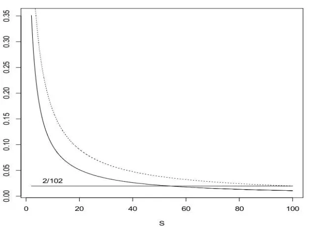
_d (see, for example Ibragimov and Khasminskii, 1980, 1981, 1982), seen as a collection of regression functions over[0,1]d_{, not}_[0,1]S_{. However, in our setting, the intrinsic dimension of the}

regression problem is S, not d, and the random forests estimate cleverly adapts to the sparsity of the problem. As an illustration, Figure 1 shows the plot of the function S7→0.75/(S log 2+0.75)for S ranging from 2 to d=100.

It is noteworthy that the rate of convergence of theξn jto 0 (and, consequently, the rate at which

the probabilities pn j approach 1/S for j∈

S

) will eventually depend on the ambient dimension d

through the ratio S/d. The same is true for the Lipschitz constant L and the factor sup_x_∈[0_,_1]dr2(x)

(9)

Figure 1: Solid line: Plot of the function S7→0.75/(S log 2+0.75)for S ranging from 2 to d=100.

Dotted line: Plot of the minimax rate power S7→2/(S+2). The horizontal line shows the value of the d-dimensional rate power 2/(d+2)≈0.0196.

contained inRS_{, so that the later supremum (respectively, the Lipschitz constant) is in fact a}

supre-mum (respectively, a Lipschitz constant) overRS_{, not over}_Rd_{. Next, denote by}

_C

p(s)the collection

of functionsη:[0,1]p_→_[0,1]_{for which each derivative of order s satisfies a Lipschitz condition.}

It is well known that the ε-entropy log₂(

N

_ε) of

C

_p(s) is Φ(ε−p/(s+1)) asε↓0 (Kolmogorov and Tihomirov, 1961), where an=Φ(bn) means that an =

O

(bn) and bn=

O

(an). Here we have an

interesting interpretation of the dimension reduction phenomenon: Working with Lipschitz func-tions on RS _{(that is, s}₌_{0) is roughly equivalent to working with functions on}Rd _{for which all}

[(d/S)−1]-th order derivatives are Lipschitz! For example, if S=1 and d=25, (d/S)−1=24 and, as there are 2524such partial derivatives inR25_{, we note immediately the potential benefit of}

recovering the “true” dimension S.

Remark 7 The reduced-dimensional rate nS log 2−0.+750.75 _{is strictly larger than the S-dimensional optimal}

rate n−2/(S+2), which is also shown in Figure 1 for S ranging from 2 to 100. We do not know whether the latter rate can be achieved by the algorithm.

Remark 8 The optimal parameter knof Corollary 6 depends on the unknown distribution of(X,Y),

especially on the smoothness of the regression function and the effective dimension S. To correct this situation, adaptive (i.e., data-dependent) choices of kn, such as data-splitting or cross-validation,

(10)

belief that this procedure should also preserve the rate of convergence, even for overfitted trees (kn≈n), in the spirit of Biau et al. (2010). However, such a study is beyond the scope of the present

paper.

Remark 9 For further references, it is interesting to note that Proposition 2 (variance term) is a consequence of aggregation, whereas Proposition 4 (bias term) is a consequence of randomization. It is also stimulating to keep in mind the following analysis, which has been suggested to us by a referee. Suppose, to simplify, that Y=r(X)(no-noise regression) and that∑_in₌₁Wni(X,Θ) =1 a.s.

In this case, the variance term is 0 and we have

¯rn(X) =˜rn(X) = n

∑

i=1

E_Θ_[_W_ni(Θ,_X_)]_Y_i_.

Set Zn= (Y,Y1, . . . ,Yn). Then

E_[¯r_n₍_X₎₋_r₍_X_)]2₌E_[¯r_n₍_X₎₋_Y_]2

=EhEh₍_¯r_n₍_X₎₋_Y₎2_|Z_nii

=EhEh₍_¯r_n₍_X₎₋E_[¯r_n₍_X₎_|Z_n_])2_|_Z_nii₊E_[E_[¯r_n₍_X₎_|Z_n_]₋_Y_]2_.

The conditional expectation in the first of the two terms above may be rewritten under the form

E

Cov E_Θ_[_r_n₍_X_,Θ)]_,E_Θ′r_n(X,Θ′)|Z_n,

whereΘ′is distributed as, and independent of,Θ. Attention shows that this last term is indeed equal to

EE_Θ_,_Θ′Cov r_n(X,Θ),r_n(X,Θ′)|Z_n.

The key observation is that if trees have strong predictive power, then they can be unconditionally strongly correlated while being conditionally weakly correlated. This opens an interesting line of research for the statistical analysis of the bias term, in connection with Amit (2002) and Blanchard (2004) conditional covariance-analysis ideas.

3. Discussion

The results which have been obtained in Section 2 rely on appropriate behavior of the probability sequences(pn j)n≥1, j=1, . . . ,d. We recall that these sequences should be in(0,1) and obey the

constraints pn j= (1/S)(1+ξn j)for j∈

S

(and pn j=ξn jotherwise), where the(ξn j)n≥1 tend to 0

as n tends to infinity. In other words, at each step of the construction of the individual trees, the random procedure should track and preferentially cut the strong coordinates. In this more informal section, we briefly discuss a random mechanism for inducing such probability sequences.

Suppose, to start with an imaginary scenario, that we already know which coordinates are strong, and which are not. In this ideal case, the random selection procedure described in the introduction may be easily made more precise as follows. A positive integer Mn—possibly depending on n—is

fixed beforehand and the following splitting scheme is iteratively repeated at each node of the tree:

(11)

2. If the selection is all weak, then choose one at random to split on. If there is more than one strong variable elected, choose one at random and cut.

Within this framework, it is easy to see that each coordinate in

S

will be cut with the “ideal” proba-bility

p⋆_n= 1

S "

1−

1−S

d Mn#

.

Though this is an idealized model, it already gives some information about the choice of the param-eter Mn, which, in accordance with the results of Section 2 (Corollary 6), should satisfy

1−S

d Mn

log n→0 as n→∞.

This is true as soon as

Mn→∞ and

Mn

log n→∞ as n→∞.

This result is consistent with the general empirical finding that Mn (calledmtry in the R package

RandomForests) does not need to be very large (see, for example, Breiman, 2001), but not with the widespread belief that Mn should not depend on n. Note also that if the Mn features are chosen at

random without replacement, then things are even more simple since, in this case, p⋆_n=1/S for all n large enough.

In practice, we have only a vague idea about the size and content of the set

S

. However, to circumvent this problem, we may use the observations of an independent second set

D

′

n (say, of

the same size as

D

_n)in order to mimic the ideal split probability p⋆_n. To illustrate this mechanism, suppose—to keep things simple—that the model is linear, that is,

Y=

∑

j∈S

ajX(j)+ε,

where X= (X(1), . . . ,X(d)₎_{is uniformly distributed over}_[0,1]d_{, the a}

j are non-zero real numbers,

andεis a zero-mean random noise, which is assumed to be independent of X and with finite vari-ance. Note that, in accordance with our sparsity assumption, r(X) =∑_j_∈SajX(j)depends on XS

only.

Assume now that we have done some splitting and arrived at a current set of terminal nodes. Consider any of these nodes, say A=∏d_j₌₁Aj, fix a coordinate j ∈ {1, . . . ,d}, and look at the

weighted conditional varianceV_[_Y_|_X(j)_∈_A_j_]P₍_X(j)_∈_A_j_{). It is a simple exercise to prove that if X}

is uniform and j∈

S

, then the split on the j-th side which most decreases the weighted conditional variance is at the midpoint of the node, with a variance decrease equal to a2_j/16>0. On the other hand, if j∈

W

, the decrease of the variance is always 0, whatever the location of the split.

On the practical side, the conditional variances are of course unknown, but they may be esti-mated by replacing the theoretical quantities by their respective sample estimates (as in the CART procedure, see Breiman, 2001, Chapter 8, for a thorough discussion) evaluated on the second sample

D

_n′. This suggests the following procedure, at each node of the tree:

(12)

2. For each of the Mn elected coordinates, calculate the best split, that is, the split which most

decreases the within-node sum of squares on the second sample

D

_n′.

3. Select one variable at random among the coordinates which output the best within-node sum of squares decreases, and cut.

This procedure is indeed close to what the random forests algorithm does. The essential dif-ference is that we suppose to have at hand a second sample

D

′

n, whereas the original algorithm

performs the search of the optimal cuts on the original observations

D

_n. This point is important, since the use of an extra sample preserves the independence ofΘ(the random mechanism) and

D

_n

(the training sample). We do not know whether our results are still true ifΘ depends on

D

_n (as in the CART algorithm), but the analysis does not appear to be simple. Note also that, at step 3, a threshold (or a test procedure, as suggested in Amaratunga et al., 2008) could be used to choose among the most significant variables, whereas the actual algorithm just selects the best one. In fact, depending on the context and the actual cut selection procedure, the informative probabilities pn j

( j∈

S

) may obey the constraints pn j→pjas n→∞(thus, pjis not necessarily equal to 1/S), where

the pj are positive and satisfy∑j∈Spj=1. This should not affect the results of the article.

This empirical randomization scheme leads to complicate probabilities of cuts which, this time, vary at each node of each tree and are not easily amenable to analysis. Nevertheless, observing that the average number of cases per terminal node is about n/kn, it may be inferred by the law of large

numbers that each variable in

S

will be cut with probability

pn j≈

1

S "

1−

1−S

d Mn#

(1+ζn j),

whereζn jis of the order

O

(kn/n), a quantity which anyway goes fast to 0 as n tends to infinity. Put

differently, for j∈

S

,

pn j≈

1

S(1+ξn j),

where ξn j goes to 0 and satisfies the constraint ξn jlog n → 0 as n tends to infinity, provided

knlog n/n→0, Mn→ ∞ and Mn/log n→ ∞. This is coherent with the requirements of

Corol-lary 6. We realize however that this is a rough approach, and that more theoretical work is needed here to fully understand the mechanisms involved in CART and Breiman’s original randomization process.

It is also noteworthy that random forests use the so-called out-of-bag samples (i.e., the boot-strapped data which are not used to fit the trees) to construct a variable importance criterion, which measures the prediction strength of each feature (see, e.g., Genuer et al., 2010). As far as we are aware, there is to date no systematic mathematical study of this criterion. It is our belief that such a study would greatly benefit from the sparsity point of view developed in the present paper, but is unfortunately much beyond its scope. Lastly, it would also be interesting to work out and extend our results to the context of unsupervised learning of trees. A good route to follow with this respect is given by the strategies outlined in Section 5.5 of Amit and Geman (1997).

4. A Small Simulation Study

(13)

random forests method, but rather to illustrate the main ideas of the article. As for now, we let

U

([0,1]d₎_{(respectively,}

_N

_{(0,1)) be the uniform distribution over}_[0,_1]d _{(respectively, the standard}

Gaussian distribution). Specifically, three models were tested:

1. [Sinus] For x∈[0,1]d_{, the regression function takes the form}

r(x) =10 sin(10πx(1)).

We let Y =r(X) +εand X∼

U

([0,1]d₎_(d_≥_{1), with}ε_∼

_N

_(0,1).

2. [Friedman #1] This is a model proposed in Friedman (1991). Here,

r(x) =10 sin(πx(1)x(2)) +20(x(3)−.05)2+10x(4)+5x(5) and Y =r(X) +ε, where X∼

U

([0,1]d₎_(d_≥_{5) and}ε_∼

_N

_(0,1).

3. [Tree] In this example, we let Y =r(X) +ε, where X∼

U

([0,1]d₎_(d_≥_5),ε_∼

_N

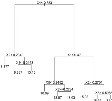
_(0,₁₎_and

the function r has itself a tree structure. This tree-type function, which is shown in Figure 2, involves only five variables.

Figure 2: The tree used as regression function in the model Tree.

We note that, although the ambient dimension d may be large, the effective dimension of model 1 is S=1, whereas model 2 and model 3 have S=5. In other words,

S

={1}for model 1, whereas

S

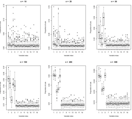
={1, . . . ,5}for model 2 and model 3. Observe also that, in our context, the model Tree should be considered as a “no-bias” model, on which the random forests algorithm is expected to perform well.

(14)

withmtry=d. For j=1, . . . ,d, the ratio (number of times the j-th coordinate is split)/(total number

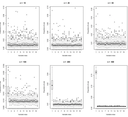
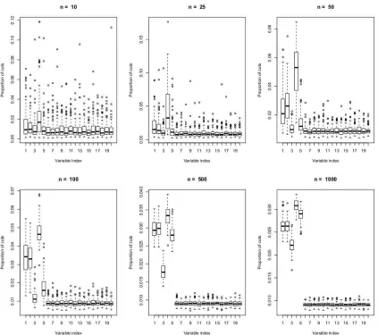
of splits over the forest) was evaluated, and the whole experiment was repeated 100 times. Figure 3, Figure 4 and Figure 5 report the resulting boxplots for each of the first twenty variables and different values of n. These figures clearly enlighten the fact that, as n grows, the probability of cuts does concentrate on the informative variables only and support the assumption thatξn j→0 as n→∞for

each j∈

S

.

Figure 3: Boxplots of the empirical probabilities of cuts for model Sinus (

S

={1}).

(15)

Figure 4: Boxplots of the empirical probabilities of cuts for model Friedman #1 (

S

={1, . . . ,5}).

approximation

MSE≈ 1

50 000

∑

j=1

[RF(test data #j)−r(test data #j)]2.

(16)

Figure 5: Boxplots of the empirical probabilities of cuts for model Tree (

S

={1, . . . ,5}).

to the original ones (samemtry, same number of random trees), with the notable difference that now

the maximum number of nodes is fixed beforehand. For the sake of coherence, since the minimum

(17)

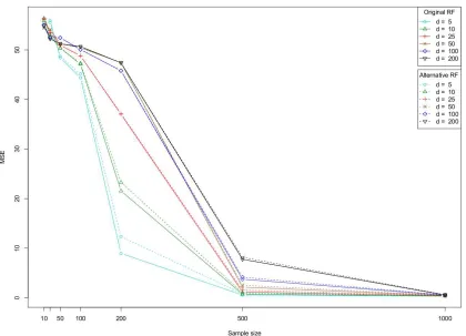
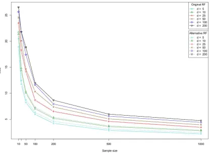
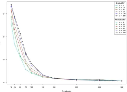
Figure 6, Figure 7 and Figure 8 illustrate the evolution of the MSE value with respect to n and

d, for each model and the two tested procedures. First, we note that the overall performance of the

alternative method is very similar to the one of the original algorithm. This confirms our idea that the model discussed in the present paper is a good approximation of the authentic Breiman’s forests. Next, we see that for a sufficiently large n, the capabilities of the forests are nearly independent of

d, in accordance with the idea that the (asymptotic) rate of convergence of the method should only

depend on the “true” dimensionality S (Theorem 5). Finally, as expected, it is noteworthy that both algorithms perform well on the third model, which has been precisely designed for a tree-structured predictor.

Figure 6: Evolution of the MSE for model Sinus (S=1).

5. Proofs

Throughout this section, we will make repeated use of the following two facts.

Fact 1 Let Kn j(X,Θ)be the number of times the terminal node An(X,Θ)is split on the j-th

(18)

Figure 7: Evolution of the MSE for model Friedman #1 (S=5).

⌈log₂kn⌉and pn j(by independence of X andΘ). Moreover, by construction, d

∑

j=1

Kn j(X,Θ) =⌈log2kn⌉.

Recall that we denote by Nn(X,Θ)the number of data points falling in the same cell as X, that is,

Nn(X,Θ) = n

∑

i=1

1_[_X_i_∈_A_n₍_X_,_Θ_)].

Letλbe the Lebesgue measure on[0,1]d_.

Fact 2 By construction,

λ(An(X,Θ)) =2−⌈log2kn⌉.

In particular, if X is uniformly distributed on[0,1]d_{, then the distribution of N}

n(X,Θ)conditionally

(19)

Figure 8: Evolution of the MSE for model Tree (S=5).

Remark 10 If X is not uniformly distributed but has a probability density f on[0,1]d_{, then,}

con-ditionally on X andΘ, Nn(X,Θ)is binomial with parameters n andP(X1∈An(X,Θ)|X,Θ). If f

is bounded from above and from below, this probability is of the orderλ(An(X,Θ)) =2−⌈log2kn⌉,

and the whole approach can be carried out without difficulty. On the other hand, for more general densities, the binomial probability depends on X, and this makes the analysis significantly harder.

5.1 Proof of Theorem 1

Observe first that, by Jensen’s inequality,

E_[¯r_n₍_X₎₋_r₍_X_)]2₌E_[E_Θ_[_r_n₍_X_,Θ)₋_r₍_X_)]]2

≤E_[_r_n₍_X,Θ)₋_r₍_X_)]2_.

A slight adaptation of Theorem 4.2 in Gy¨orfi et al. (2002) shows that ¯rn is consistent if both

diam(An(X,Θ))→0 in probability and Nn(X,Θ)→∞in probability.

Let us first prove that Nn(X,Θ)→∞in probability. To see this, consider the random tree

parti-tion defined byΘ, which has by construction exactly 2⌈log2kn⌉_{rectangular cells, say A}

(20)

Let N1, . . . ,N₂⌈_{log2 kn}⌉denote the number of observations among X,X1, . . . ,Xnfalling in these 2⌈log2kn⌉

cells, and let

C

={X,X1, . . . ,Xn}denote the set of positions of these n+1 points. Since these points

are independent and identically distributed, fixing the set

C

andΘ, the conditional probability that

X falls in theℓ-th cell equals Nℓ/(n+1). Thus, for every fixed M≥0,

P₍_N_n₍_X,Θ)_<_M_{) =}E_[P₍_N_n₍_X,Θ)_<_M_|C,Θ)]

=E





∑

ℓ=1,...,2⌈log2 kn⌉_:N

ℓ<M

Nℓ n+1





≤M2 ⌈log2kn⌉

n+1

≤2Mkn n+1,

which converges to 0 by our assumption on kn.

It remains to show that diam(An(X,Θ))→0 in probability. To this aim, let Vn j(X,Θ)be the size

of the j-th dimension of the rectangle containing X. Clearly, it suffices to show that Vn j(X,Θ)→0

in probability for all j=1, . . . ,d. To this end, note that

Vn j(X,Θ)

D

=2−Kn j(X,Θ)_,

where, conditionally on X, Kn j(X,Θ)has a binomial

B

(⌈log2kn⌉,pn j)distribution, representing the

number of times the box containing X is split along the j-th coordinate (Fact 1). Thus

E_[_V_{n j}₍_X_,Θ)] =Eh₂−Kn j(X,Θ)

i

=EhEh₂−Kn j(X,Θ)_|Xii

= (1−pn j/2)⌈log2kn⌉,

which tends to 0 as pn jlog kn→∞.

5.2 Proof of Proposition 2

Recall that

¯rn(X) = n

∑

i=1

E_Θ_[_W_ni₍_X,Θ)]_Y_i_,

where

Wni(X,Θ) =

1[Xi∈An(X,Θ)]

Nn(X,Θ)

1En(X,Θ)

and

E

n= [Nn(X,Θ)6=0].

Similarly,

˜rn(X) = n

∑

i=1

(21)

We have

E_[¯r_n₍_X₎₋_˜r_n₍_X_)]2₌E

"

n

∑

i=1

E_Θ_[_W_ni₍_X,Θ)] (_Y_i₋_r₍_X_i₎₎

#2

=E

"

n

∑

i=1

E2_Θ_[_W_ni₍_X,Θ)] (_Y_i₋_r₍_X_i₎₎2

#

(the cross terms are 0 sinceE_[_Y_i_|X_i_{] =}_r₍_X_i₎₎

=E

"

n

∑

i=1

E2_Θ_[_W_ni₍_X,Θ)]σ2₍_X_i₎

#

≤σ2_E

"

n

∑

i=1

E2_Θ_[_W_ni₍_X,Θ)]

#

=nσ2E

E2_Θ_[_W_n1₍_X_,Θ)] ,

where we used a symmetry argument in the last equality. Observe now that

E2_Θ_[_W_n1₍_X,Θ)] =E_Θ_[_W_n1₍_X_,Θ)]E_Θ′W_n1(X,Θ′)

(whereΘ′is distributed as, and independent of,Θ) =E_Θ_,_Θ′W_n1(X,Θ)W_n1(X,Θ′)

=E_Θ_,_Θ′ ₁

[X1∈An(X,Θ)]1[X1∈An(X,Θ′)]

Nn(X,Θ)Nn(X,Θ′)

1En(X,Θ)1En(X,Θ′)

=E_Θ_,_Θ′ ₁

[X1∈An(X,Θ)∩An(X,Θ′)]

Nn(X,Θ)Nn(X,Θ′)

.

Consequently,

E_[¯r_n₍_X₎₋_˜r_n₍_X_)]2_≤_nσ2E

₁

[X1∈An(X,Θ)∩An(X,Θ′)]

Nn(X,Θ)Nn(X,Θ′)

(22)

Therefore

E_[¯r_n₍_X₎₋_˜r_n₍_X_)]2

≤nσ2E

"

1[X1∈An(X,Θ)∩An(X,Θ′)]

1+∑n_i₌₂1[Xi∈An(X,Θ)]

1+∑n_i₌₂1[Xi∈An(X,Θ′)]

#

=nσ2E

"

E

"

1_[X1∈An(X,Θ)∩An(X,Θ′)]

1+∑n_i₌₂1[Xi∈An(X,Θ)]

× 1

1+∑n_i₌₂1[Xi∈An(X,Θ′)]

|X,X1,Θ,Θ

′

##

=nσ2E

"

1[X1∈An(X,Θ)∩An(X,Θ′)]E

"

1

1+∑n_i₌₂1[Xi∈An(X,Θ)]

× 1

1+∑n

i=21[Xi∈An(X,Θ′)]

|X,X1,Θ,Θ

′

##

=nσ2E

"

1[X1∈An(X,Θ)∩An(X,Θ′)]E

"

1 1+∑n

i=21[Xi∈An(X,Θ)]

× 1

1+∑n

|X,Θ,Θ

′

##

by the independence of the random variables X,X1, . . . ,Xn,Θ,Θ′. Using the Cauchy-Schwarz

in-equality, the above conditional expectation can be upper bounded by

E1/2

"

1

1+∑n

i=21[Xi∈An(X,Θ)]

2|X,Θ #

×E1/2

"

1

1+∑n

2|X,Θ

′

#

≤3×2 2⌈log2kn⌉

n2

(by Fact 2 and technical Lemma 11)

≤12k 2

n

n2 .

It follows that

E_[¯r_n₍_X₎₋_˜r_n₍_X_)]2_≤12σ

2_k2

n

n E

1[X1∈An(X,Θ)∩An(X,Θ′)]

=12σ

2_k2

n n E E_X 1

1_[X1∈An(X,Θ)∩An(X,Θ′)]

=12σ

2_k2

n

n E

P_X

1 X1∈An(X,Θ)∩An(X,Θ

′₎

. (3)

Next, using the fact that X1is uniformly distributed over[0,1]d, we may write

P_X

1 X1∈An(X,Θ)∩An(X,Θ

′₎

=λ An(X,Θ)∩An(X,Θ′)

=

d

∏

j=1

λ An j(X,Θ)∩An j(X,Θ′)

(23)

where

An(X,Θ) = d

∏

j=1

An j(X,Θ) and An(X,Θ′) = d

∏

j=1

An j(X,Θ′).

On the other hand, we know (Fact 1) that, for all j=1, . . . ,d,

λ(An j(X,Θ))

D

=2−Kn j(X,Θ)_,

B

(⌈log2kn⌉,pn j)distribution and, similarly,

λ An j(X,Θ′)

D

=2−Kn j′ (X,Θ′)_,

where, conditionally on X, K_{n j}′ (X,Θ′₎_{is binomial}

_B

₍_⌈_log

2kn⌉,pn j)and independent of Kn j(X,Θ).

In the rest of the proof, to lighten notation, we write Kn jand Kn j′ instead of Kn j(X,Θ)and Kn j′ (X,Θ′),

respectively. Clearly,

≤2−max(Kn j,Kn j′ )

=2−Kn j′ ₂−(Kn j−Kn j′ )+

and, consequently,

d

∏

j=1

≤2−⌈log2kn⌉

d

∏

j=1

2−(Kn j−Kn j′ )+

(since, by Fact 1, ∑d_j₌₁Kn j =⌈log2kn⌉). Plugging this inequality into (3) and applying H¨older’s

inequality, we obtain

E_[¯r_n₍_X₎₋_˜r_n₍_X_)]2_≤12σ

2_k n n E " d

∏

j=1

2−(Kn j−Kn j′ )+

# =12σ 2_k n n E " E " d

∏

j=1

2−(Kn j−Kn j′ )+_|_X

## ≤12σ 2_k n n E " d

∏

j=1

E1/dh₂−d(Kn j−Kn j′ )+_|Xi

# .

Each term in the product may be bounded by technical Proposition 13, and this leads to

E_[¯r_n₍_X₎₋_˜r_n₍_X_)]2_≤288σ

2_k n πn d

∏

j=1 min 1, π

16⌈log₂kn⌉pn j(1−pn j)

1/2d!

≤288σ 2_k n πn d

∏

j=1 min 1, π log 2

16(log kn)pn j(1−pn j)

1/2d! .

Using the assumption on the form of the pn j, we finally conclude that

E_[¯r_n₍_X₎₋_˜r_n₍_X_)]2_≤_Cσ2

S2 S−1

S/2d

(1+ξn)

kn

n(log kn)S/2d

(24)

where

C=288 π

πlog 2

16

S/2d

and

1+ξn=

∏

j∈S

"

(1+ξn j)−1

1− ξn j S−1

−1#1/2d .

Clearly, the sequence (ξn), which depends on the {(ξn j): j ∈

S

} only, tends to 0 as n tends to

infinity.

5.3 Proof of Proposition 4

We start with the decomposition

E_[˜r_n₍_X₎₋_r₍_X_)]2

=E

"

n

∑

i=1

E_Θ_[_W_ni₍_X,Θ)] (_r₍_X_i₎₋_r₍_X_{)) +} n

∑

i=1

E_Θ_[_W_ni₍_X_,Θ)]₋₁

!

r(X) #2 =E " E_Θ " n

∑

i=1

Wni(X,Θ) (r(Xi)−r(X)) + n

∑

i=1

Wni(X,Θ)−1

!

r(X) ##2 ≤E " n

∑

i=1

Wni(X,Θ) (r(Xi)−r(X)) + n

∑

i=1

Wni(X,Θ)−1

!

r(X) #2

,

where, in the last step, we used Jensen’s inequality. Consequently,

E_[˜r_n₍_X₎₋_r₍_X_)]2

≤E

"

n

∑

i=1

Wni(X,Θ) (r(Xi)−r(X))

#2

+E_r₍_X₎₁_Ec n(X,Θ)

2 ≤E " n

∑

i=1

#2 +

"

sup

x∈[0,1]d

r2(x) #

P₍

E

c

(25)

Let us examine the first term on the right-hand side of (4). Observe that, by the Cauchy-Schwarz inequality, E " n

∑

i=1

#2 ≤E " n

∑

i=1 p

Wni(X,Θ)

p

Wni(X,Θ)|r(Xi)−r(X)|

#2 ≤E " n

∑

i=1

Wni(X,Θ)

!

n

∑

i=1

Wni(X,Θ) (r(Xi)−r(X))2

!# ≤E " n

∑

i=1

Wni(X,Θ) (r(Xi)−r(X))2

#

(since the weights are subprobability weights).

Thus, denoting bykXkS the norm of X evaluated over the components in

S

, we obtain

E

"

n

∑

i=1

#2 ≤E " n

∑

i=1

Wni(X,Θ) (r⋆(XiS)−r⋆(XS))2

#

≤L2

n

∑

i=1

E_W_ni₍_X_,Θ)_kX_i₋_Xk2_S

=nL2E_W_n1₍_X,Θ)_kX₁₋_Xk2_S

(by symmetry).

But

E_W_n1₍_X_,Θ)_kX1₋_Xk2_S

=E

kX1−Xk2S

1_[_X₁_∈_A_n₍_X_,_Θ_)] Nn(X,Θ)

1En(X,Θ)

=E

kX1−Xk2S

1[X1∈An(X,Θ)]

1+∑n

i=21[Xi∈An(X,Θ)]

=E

E

kX1−Xk2S

1[X1∈An(X,Θ)]

1+∑n_i₌₂1[Xi∈An(X,Θ)]

|X,X1,Θ

.

Thus,

E

Wn1(X,Θ)kX1−Xk2S

=E

kX1−Xk2S1[X1∈An(X,Θ)]E

1 1+∑n

i=21[Xi∈An(X,Θ)]

|X,X1,Θ

=E

kX1−Xk2S1[X1∈An(X,Θ)]E

1

1+∑n_i₌₂1[Xi∈An(X,Θ)] |X,Θ

(26)

By Fact 2 and technical Lemma 11,

E

1 1+∑n

i=21[Xi∈An(X,Θ)] |X,Θ

≤2 ⌈log2kn⌉

n ≤ 2kn n . Consequently, E " n

∑

i=1

#2

≤2L2knE

kX1−Xk2S1[X1∈An(X,Θ)]

.

Letting

An(X,Θ) = d

∏

j=1

An j(X,Θ),

we obtain E " n

∑

i=1

#2

≤2L2kn

∑

j∈S

Eh_|X(j)

1 −X(j)|21[X1∈An(X,Θ)]

i

=2L2kn

∑

j∈S

E

h

ρj(X,X1,Θ)E_X(j)

1

h

|X(₁j)−X(j)|21

[X(1j)∈An j(X,Θ)]

ii

where, in the last equality, we set

ρj(X,X1,Θ) =

∏

t=1,...,d,t6=j

1_[_X(t)

1 ∈Ant(X,Θ)].

Therefore, using the fact that X1is uniformly distributed over[0,1]d,

E

"

n

∑

i=1

#2

≤2L2kn

∑

j∈S

Eρ

j(X,X1,Θ)λ3(An j(X,Θ))

.

Observing that

λ(An j(X,Θ))×E_[_X(t)

1 :t=1,...,d,t6=j]

[ρj(X,X1,Θ)]

=λ(An(X,Θ))

=2−⌈log2kn⌉

(Fact 2),

we are led to

E

"

n

∑

i=1

#2

≤2L2

∑

j∈S

Eλ₂

(An j(X,Θ))

=2L2

∑

j∈S

Eh₂−2Kn j(X,Θ)i

=2L2

∑

j∈S

E

h

E

h

2−2Kn j(X,Θ)_|_X

(27)

B

(⌈log2kn⌉,pn j)distribution (Fact 1).

Conse-quently,

E

"

n

∑

i=1

#2

≤2L2

∑

j∈S

(1−0.75pn j)⌈log2kn⌉

≤2L2

∑

j∈S

exp

−0.75

log 2pn jlog kn

=2L2

∑

j∈S

1

k

0.75

S log 2(1+ξn j)

n

≤ 2SL 2 k

0.75

S log 2(1+γn)

n

,

withγn=minj∈Sξn j.

To finish the proof, it remains to bound the second term on the right-hand side of (4), which is easier. Just note that

P₍

E

c

n(X,Θ)) =P n

∑

i=1

1_[_X_i_∈_A_n₍_X_,_Θ_)]=0 !

=E

"

P n

∑

i=1

1_[_X_i_∈_A_n₍_X_,_Θ_)]=0|X,Θ

!#

=1−2−⌈log2kn⌉n

(by Fact 2)

≤e−n/2kn_.

Putting all the pieces together, we finally conclude that

E_[˜r_n₍_X₎₋_r₍_X_)]2_≤ 2SL

2 k

0.75

S log 2(1+γn)

n

+ "

sup

x∈[0,1]d

r2(x) #

e−n/2kn_,

as desired.

5.4 Some Technical Results

The following result is an extension of Lemma 4.1 in Gy¨orfi et al. (2002). Its proof is given here for the sake of completeness.

Lemma 11 Let Z be a binomial

B

(N,p)random variable, with p∈(0,1]. Then

(i)

E

1 1+Z

≤ 1