Message-Passing Algorithms for Quadratic Minimization

Message-Passing Algorithms for Quadratic Minimization

Nicholas Ruozzi [email protected]

Communication Theory Laboratory ´

Ecole Polytechnique F´ed´erale de Lausanne Lausanne 1015, Switzerland

Sekhar Tatikonda [email protected]

Department of Electrical Engineering Yale University

New Haven, CT 06520, USA

Editor:Martin Wainwright

Abstract

Gaussian belief propagation (GaBP) is an iterative algorithm for computing the mean (and vari-ances) of a multivariate Gaussian distribution, or equivalently, the minimum of a multivariate pos-itive definite quadratic function. Sufficient conditions, such as walk-summability, that guarantee the convergence and correctness of GaBP are known, but GaBP may fail to converge to the correct solution given an arbitrary positive definite covariance matrix. As was observed by Malioutov et al. (2006), the GaBP algorithm fails to converge if the computation trees produced by the algorithm are not positive definite. In this work, we will show that the failure modes of the GaBP algorithm can be understood via graph covers, and we prove that a parameterized generalization of the min-sum algorithm can be used to ensure that the computation trees remain positive definite whenever the input matrix is positive definite. We demonstrate that the resulting algorithm is closely related to other iterative schemes for quadratic minimization such as the Gauss-Seidel and Jacobi algorithms. Finally, we observe, empirically, that there always exists a choice of parameters such that the above generalization of the GaBP algorithm converges.

Keywords: belief propagation, Gaussian graphical models, graph covers

1. Introduction

Let Γ_∈Rn×n be a symmetric positive definite matrix and h_∈Rn. The quadratic minimization

problem is to find thex_∈Rnthat minimizes f(x) = 1

2x

T_Γx−hT_{x. Minimizing a positive definite}

quadratic function is equivalent to computing the mean of a multivariate Gaussian distribution with a positive definite covariance matrix, or equivalently, solving the positive definite linear system Γx=hfor the vectorx.

Because of the importance of solving linear systems, many different algorithms for the mini-mization of quadratic functions have been studied: Gaussian elimination, Gauss-Seidel iteration, Jacobi iteration, successive over-relaxation, etc. Distributed algorithms that can take advantage of

the sparsity of the matrixΓare particularly desirable for solving large-scale systems as even

important because they represent one of the few continuous distributions for which exact message updates can be efficiently computed and more complicated distributions are often approximated by Gaussian distributions in practice.

In previous work, several authors have provided sufficient conditions for the convergence of GaBP. Weiss and Freeman (2001b) demonstrated that GaBP converges in the case that the covari-ance matrix is diagonally dominant. Malioutov et al. (2006) proved that the GaBP algorithm con-verges when the covariance matrix is walk-summable. Moallemi and Van Roy (2009, 2010) showed that scaled diagonal dominance was a sufficient condition for convergence and also characterized the rate of convergence via a computation tree analysis. The latter two sufficient conditions, walk-summability and scaled diagonal dominance, are known to be equivalent (Malioutov, 2008; Ruozzi et al., 2009).

While the above conditions are sufficient for the convergence of the GaBP algorithm they are not necessary: there are examples of positive definite matrices that are not walk-summable for which the GaBP algorithm still converges to the correct solution (Malioutov et al., 2006). A criti-cal component of these examples is that the computation trees remain positive definite throughout the algorithm. Such behavior is guaranteed if the original matrix is scaled diagonally dominant, but arbitrary positive definite matrices can produce computation trees that are not positive definite (Malioutov et al., 2006). If this occurs, the standard GaBP algorithm fails to produce the correct solution. The purpose of this work is to understand why GaBP fails and to design iterative message-passing algorithms with improved convergence guarantees outside of the walk-summable case.

Related work studies the effect of preconditioning: the covariance matrix is preconditioned in order to force it to be scaled diagonally dominant and then the GaBP algorithm is applied to solve the preconditioned problem. Diagonal loading was proposed as one such useful preconditioner (Johnson et al., 2009). The key insight of diagonal loading is that scaled diagonal dominance can be achieved by sufficiently weighting the diagonal elements of the inverse covariance matrix. The diagonally loaded matrix can then be used as an input to a GaBP subroutine. The solution produced by GaBP is then used in a feedback loop to produce a new matrix, and the process is repeated until a desired level of accuracy is achieved. The performance is determined, in part, by the amount of diagonal loading needed to make the matrix scaled diagonally dominant. However, choosing the appropriate amount of diagonal loading that achieves the fastest rate of convergence remains an open question. As the approach in this work is to study reweighted versions of GaBP, our techniques can also be applied as part of this algorithmic scheme (or by themselves), and we provide experimental evidence that this technique results in performance gains over GaBP, allowing for less diagonal loading.

algo-rithms for the quadratic minimization problem, but as we show using the theory of graph covers, iterative schemes based on dual optimization techniques that guarantee the correctness of locally decodable beliefs cannot converge to the correct minimizing assignment outside of walk-summable models.

In this work, we investigate the behavior of reweighted message-passing algorithms for the quadratic minimization problem. The motivation for this study comes from the observation that belief propagation style algorithms typically do not explore all nodes in the factor graph with the same frequency (Frey et al., 2001). In many application areas, such uneven counting is undesirable and typically results in incorrect answers, but if we can use reweighting to overestimate the diagonal entries of the computation tree relative to the off diagonal entries, then we may be able to force the computation trees to be positive definite at each iteration of the algorithm. Although similar in spirit to diagonal loading, our approach obviates the need for preconditioning. We will show that there exists a choice of parameters for the reweighted algorithms that guarantees monotone convergence of the variance estimates on all positive definite models, even those for which the GaBP algorithm fails to converge. We empirically observe that there exists a choice of parameters that also guarantees the convergence of the mean estimates. In addition, we show that our graph cover analysis extends to other iterative algorithms for the quadratic minimization problem and that similar ideas can be used to reason about the min-sum algorithm for general convex minimization.

The outline of this paper is as follows. In Section 2 we review the min-sum algorithm, its reweighted generalizations, and the quadratic minimization problem. In Section 3 we discuss the relationship between pairwise message-passing algorithms and graph covers, and we show how to use graphs covers to characterize walk-summability. In Section 4, we examine the convergence of the means and the variances under the reweighted algorithm for the quadratic minimization problem, we explore the relationship between the reweighted algorithm and the Gauss-Seidel and Jacobi methods, and we compare the performance of the reweighted algorithm to the standard min-sum algorithm. Finally, in Section 5, we summarize the results and discuss extensions of this work to general convex functions as well as open problems. Detailed proofs of the two main theorems can be found in Appendices A and B.

2. Preliminaries

In this section, we review the min-sum algorithm and a reweighted variant over pairwise factor graphs. Of particular importance for later proofs will be the computation trees generated by each of these algorithms. We also review the quadratic minimization problem, and explain the closed-form message updates for this problem.

2.1 The Min-Sum Algorithm

The min-sum algorithm attempts to compute the minimizing assignment of an objective function f :∏i

X

potentials as follows.

f(x1, ...,xn) =

∑

φi(xi) +

∑

(i,j)∈E

ψi j(xi,xj)

We assume that this minimization problem is well-defined: f is bounded from below and there

x1

x2 x3

ψ12 ψ13

ψ23

(a) Factor graph.

x1

x2 x3

ψ12 ψ13

ψ23 (b) The graphG.

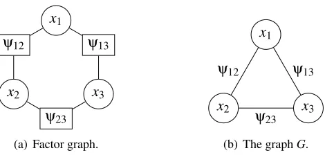
Figure 1: The factor graph corresponding to f(x1,x2,x3) =φ1+φ2+φ3+ψ12+ψ23+ψ13and the

graphG. The functionsφ1,φ2, andφ3each depend on only one variable, and are typically

omitted from the factor graph representation for clarity.

To each factorization, we associate a bipartite graph known as the factor graph. In general, the factor graph consists of a node for each of the variablesx1, ...,xn, a node for each of theψi j, and

for all(i,j)_∈E, an edge joining the node corresponding to xi to the node corresponding toψi j.

Because theψi j each depend on exactly two factors, we often omit the factor nodes from the factor

graph construction and replace them with a single edge. This reduces the factor graph to the graph

G. See Figure 1 for an example of this construction.

We can write the min-sum algorithm as a local message-passing algorithm over the graph G.

During the execution of the min-sum algorithm, messages are passed back and forth between

adja-cent nodes of the graph. On thetthiteration of the algorithm, messages are passed along each edge

of the factor graph as

mt_i→j(xj) = κ+min xi

h

ψi j(xi,xj) +φi(xi) +

∑

mt_k−_→1_i(xi)

i

,

where ∂i denotes the set of neighbors of the node i in G and ∂j_\i is abusive notation for the

set-theoretic difference∂j_{\ {}i_}. When the factor graph is a tree, these updates are guaranteed to

converge, but understanding when these updates converge to the correct solution for an arbitrary graph is a central question underlying the study of the min-sum algorithm.

Each message update has an arbitrary normalization factorκ. Becauseκis not a function of any

of the variables, it only affects the value of the minimum and not where the minimum is located. As such, we are free to choose it however we like for each message and each time step. In practice, these constants are used to avoid numerical issues that may arise during the execution of the algorithm.

We will think of the messages as a vector of functions indexed by the edge over which the message is passed. Any vector of real-valued messages is a valid choice for the vector of initial

messagesm0, and the choice of initial messages can greatly affect the behavior of the algorithm. A

typical assumption, that we will use in this work, is that the initial messages are chosen such that m0_i→j≡0 for alliand j.

Given any vector of messages,mt, we can construct a set of beliefs that are intended to

approx-imate the min-marginals of f as

τt_i(xi) = κ+φi(xi) +

∑

mt_j→i(xi),

Additionally, we can approximate the optimal assignment by computing an estimate of the argmin,

xt_{i ∈} arg min

xi

τt_i(xi).

If the beliefs are equal to the true min-marginals of f (i.e.,τt

i(xi) =minx′_:x′

i=xi f(x′)), then for

anyyi∈arg minxiτ

t

i(xi)there exists a vectorx∗such thatx∗i =yiandx∗minimizes the function f. If

|arg minxiτ

t

i(xi)|=1 for alli, then we can takex∗=y, but, if the objective function has more than

one optimal solution, then we may not be able to construct such anx∗so easily.

Definition 1 A vector,τ= (_{τi},{τi j}), of beliefs islocally decodableto x∗ifτi(x∗i)<τi(xi)for all i, xi6=x∗i. Equivalently, for each i∈V ,τiis uniquely minimized at x∗i.

If the algorithm converges to a vector of beliefs that are locally decodable tox∗, then we hope

that the vector x∗ is a global minimum of the objective function. This is indeed the case when

the factor graph contains no cycles (Wainwright et al., 2004) but need not be the case for arbitrary graphical models.

2.1.1 COMPUTATIONTREES

An important tool in the analysis of the min-sum algorithm is the notion of a computation tree. Intu-itively, the computation tree is an unrolled version of the original graph that captures the evolution of

the messages passed by the min-sum algorithm needed to compute the belief at timetat a particular

node of the factor graph. Computation trees describe the evolution of the beliefs over time, which, in some cases, can help us prove correctness and/or convergence of the message-passing updates. For example, the convergence of the min-sum algorithm on graphs containing a single cycle can be demonstrated by analyzing the computation trees produced by the min-sum algorithm at each time step (Weiss, 2000).

The depthtcomputation tree rooted at nodeicontains all of the lengthtnon-backtracking walks

in the factor graph starting at nodei. A walk is non-backtracking if it does not go back and forth

successively between two vertices. For any nodevin the factor graph, the computation tree at time

trooted ati, denoted byTi(t), is defined recursively as follows. Ti(0)is just the nodei, the root of

the tree. The treeTi(t)at timet>0 is generated fromTi(t−1)by adding to each leaf ofTi(t−1)

a copy of each of its neighbors inG(and the corresponding edge), except for the neighbor that is

already present inTi(t−1). Each node ofTi(t)is a copy of a node inG, and the potentials on the

nodes in Ti(t), which operate on a subset of the variables inTi(t), are copies of the potentials of

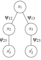
the corresponding nodes inG. The construction of a computation tree for the graph in Figure 1 is

pictured in Figure 2. Note that each variable node inTi(t)represents a distinct copy of some variable xj in the original graph.

Given any initialization of the messages, Ti(t) captures the information available to nodeiat

timet. At timet=0, node ihas received only the initial messages from its neighbors, soTi(0)

consists only ofi. At timet=1,ireceives the round one messages from all of its neighbors, soi’s

neighbors are added to the tree. These round one messages depend only on the initial messages, so the tree terminates at this point. By construction, we have the following lemma.

x1

x2

x′₃

x3

x′₂

ψ12 ψ13

ψ23 ψ23

Figure 2: The computation tree at timet=2 rooted at the variable nodex1of the graph in Figure 1.

The self-potentials corresponding to each variable node are given by the subscript of the variable.

Proof Tatikonda and Jordan (2002) and Weiss and Freeman (2001a) both provide a proof of this lemma.

Computation trees provide a dynamic view of the min-sum algorithm. After a finite number of time steps, we hope that the beliefs at the root of the computation trees stop changing and that the message vector converges to a fixed point of the message update equations (in practice, when the beliefs change by less than some small amount, we say that the algorithm has converged). For any real-valued objective function f (i.e.,_|f(x)_|<∞for allx), there always exists a fixed point of the message update equations (see Theorem 2 of Wainwright et al. 2004).

2.2 Reweighted Message-Passing Algorithms

Because the min-sum algorithm is not guaranteed to converge and, even it does, is not guaranteed to compute the correct minimizing assignment, recent research has focused on the design of alternative message-passing schemes that do not suffer from these drawbacks. Efforts to produce provably convergent message-passing schemes have resulted in the reweighted message-passing algorithm described in Algorithm 1. This algorithm is parameterized by a vector of non-zero real weights for

each edge of the graph. Notice that if we set ci j =1 for all iand j, then we obtain the standard

min-sum algorithm. Wainwright et al. (2005) choose theci j in a specific way in order to guarantee

correctness of the algorithm (which they call TRMP in this special case). In this work, we will focus on choices of these weights that will guarantee convergence of the algorithm for the quadratic minimization problem. These choices will, surprisingly, not coincide with those of the TRMP algorithm. In fact, the choice of weights that guarantees correctness of the TRMP algorithm must necessarily cause the algorithm to either not converge or converge to the incorrect solution whenever the given matrix is not walk-summable.

The beliefs for the reweighted algorithm are defined analogously to those for the standard min-sum algorithm.

τt_i(xi) = κ+φi(xi) +

∑

cjimtj→i(xi),

τt_{i j}(xi,xj) = κ+

ψi j(xi,xj) ci j

Algorithm 1Synchronous Reweighted Message-Passing Algorithm

1: Initialize the messages to some finite vector.

2: For iterationt=1,2, ...update the the messages as follows:

mt_i→j(xj):=κ+min xi

h_{ψi j(xi,xj)}

ci j

+φi(xi) + (ci j−1)mtj−→1i(xi) +

∑

ckimtk−_→1i(xi)

i

.

The vector of messages at any fixed point of the message update equations has two important properties. First, the beliefs corresponding to these messages provide an alternative factorization of

the objective function f. Second, the beliefs correspond to approximate marginals.

Lemma 3 For any vector of messages mt with corresponding beliefsτt_,

f(x1, . . . ,x_|V|) =κ+

∑

i_∈V

τt_i(xi) +

∑

(i,j)∈E ci j

h

τt_{i j}(xi,xj)−τit(xi)−τtj(xj)

i

.

Lemma 4 Ifτis a set of beliefs corresponding to a fixed point of the message updates in Algorithm 1, then

min

xj

τi j(xi,xj) =κ+τi(xi)

for all(i,j)_∈G and all xi.

The proof of these two lemmas is a straightforward exercise in applying the definitions. Wain-wright et al. (2004) provide similar results for the special case of the max-product algorithm.

2.2.1 COMPUTATIONTREES

The computation trees produced by Algorithm 1 are different from their predecessors. Again, the

computation tree captures the messages that would need to be passed in order to computeτt

i(xi).

However, the messages that are passed in the new algorithm are multiplied by a non-zero constant.

As a result, the potential at a nodeu in the computation tree corresponds to some potential in the

original graph multiplied by a constant that depends on all of the nodes aboveuin the computation

tree. We summarize the changes as follows.

1. The message passed fromito jmay now depend on the message from jtoiat the previous

time step. As such, we now form the timet+1 computation tree from the timetcomputation

tree by taking any leafu, which is a copy of nodev in the factor graph, of the timet

com-putation tree, creating a new node for everyw_∈∂v, and connecting uto these new nodes.

As a result, the new computation tree rooted at nodeuof depthtcontains at least all of the

non-backtracking walks of lengthtin the factor graph starting fromuand, at most, all walks

of lengthtin the factor graph starting atu.

2. The messages are weighted by the elements of c. This changes the potentials at the nodes

x1 φ1

x2 c12φ2

x₃′ c12c23φ3

x3 c13φ3

x′₂ c13c23φ2 x′₁

(c2₁₂₋c12)φ1 x′′₁ (c2₁₃₋c13)φ1

ψ12 ψ13

ψ23c12

c13

ψ12(c12−1)

c12

ψ23c13

c23

ψ13(c13−1)

c13

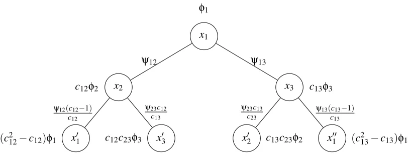
Figure 3: Construction of the computation tree rooted at nodex1at timet=2 produced by

Algo-rithm 1 for the factor graph in Figure 1. Self-potentials are adjacent to the variable node to which they correspond. One can check that settingci j=1 for all(i,j)∈Ereduces the

above computation tree to that of Figure 2.

every potential along this branch of the computation tree is multiplied byci j. To make this

concrete, we can associate a weight to every edge of the computation tree that corresponds to the constant that multiplies the message passed across that edge. To compute the new potential

at a variable node i in the computation tree, we now need to multiply the corresponding

potential φi by each of the weights corresponding to the edges that appear along the path

fromito the root of the computation tree. An analogous process can be used to compute the

potentials on each of the edges. The computation tree produced by Algorithm 1 at timet=2

for the factor graph in Figure 1 is pictured in Figure 3. Compare this with computation tree produced by the standard min-sum algorithm in Figure 2.

If we make these adjustments, then the belief, τt

i(xi), at nodeiat timet is given by the

min-marginal at the root ofTi(t). In this way, the beliefs correspond to marginals at the root of these

computation trees.

2.3 Quadratic Minimization

We now address the quadratic minimization problem in the context of the reweighted min-sum

algorithm. Recall that given a matrixΓthe quadratic minimization problem is to find the vectorx

that minimizes f(x) =1₂xTΓx₋hTx. Without loss of generality, we can assume that the matrixΓis symmetric as the quadratic function 1₂xTΓx₋hTxis equivalent to 1₂xT

h

1

2(Γ+ΓT)

i

Γ_∈Rn×n_.

f(x) = 1 2x

Th1

2(Γ+Γ

T_{) +}1

2(Γ−Γ

T₎i_x

−hTx

= 1 2x

Th1

2(Γ+Γ

T₎i_x+1

2x

Th1

2(Γ−Γ

T₎i_x

−hTx

= 1 2x

Th1

2(Γ+Γ

T₎i_x−hT_x.

Every quadratic function admits a pairwise factorization

f(x1, ...,xn) =

1 2x

T_Γx−hT_x

=

_∑

i

[1 2Γiix

2

i −hixi] +

∑

Γi jxixj,

whereΓ_∈Rn×n_{is a symmetric matrix. We note that we will abusively write min in the reweighted}

update equations even though the appropriate notion of minimization for the real numbers is inf. We can explicitly compute the minimization required by the reweighted min-sum algorithm

at each time step: the synchronous message updatemt_i→j(xj)can be parameterized as a quadratic

function of the form 1₂at_i→jx2_j+bt_i→jxj. If we define

At_i\j,

h

Γii+

∑

cki·at_k−_→1_i

i

−at_j−_→1_i

and

Bt_i\j,

h

hi−

∑

cki·bt_k−_→1_i

i

−bt_j−_→1_i,

then the updates at timetare given by

at_i→j:=−

Γi j

ci j

2

At_i\j ,

bt_i→j:=B

t i\j

Γi j

ci j

At_i\j .

These updates are only valid whenAi_\j>0. If this is not the case, then the minimization given in

Algorithm 1 is not bounded from below, and we setat_i→j =₋∞. For the initial messages, we set

a0_i→j=b0_i→j=0.

Suppose that the beliefs generated from a fixed point of Algorithm 1 are locally decodable to

x∗. One can show that the gradient of f atx∗ is always equal to zero. If the gradient of f atx∗ is

zero andΓis positive definite, thenx∗must be a global minimum off. In other words, the min-sum

algorithm always computes the correct minimizing assignment if it converges to locally decodable beliefs. This result was previously proven for the GaBP algorithm (Weiss and Freeman, 2001b) and the tree-reweighted algorithm (Wainwright et al., 2003a).

Proof For completeness, we sketch the proof. By Lemmas 3 and 4, we have that,

min

xj

τi j(xi,xj) =κ+τi(xi)

for all(i,j)_∈Gand

f(x1, . . . ,x_|V|) =κ+

∑

i∈V

τi(xi) +

∑

(i,j)∈E ci j

h

τi j(xi,xj)−τi(xi)−τj(xj)

i

.

Ifτis locally decodable tox∗, then for eachi∈V,τi(xi)must be a positive definite quadratic function

that is minimized atx∗_i. Applying Lemma 4, we have that for each(i,j)_∈E,τi j is also a positive

definite quadratic function andτi jis minimized at(x∗i,x∗j). For eachi∈V,

d dxi

f(x1, . . . ,x_|V|) =

d dxi

τi(xi) +

∑

ci j

h _d

dxi

τi j(xi,xj)− d dxi

τi(xi)

i

.

By the above arguments, for eachi_∈V,_dxd

iτi(xi)

x∗=0. Similarly, for all(i,j)∈E, d

dxiτi j(xi,xj)

x∗= 0. As a result, we must have∇f(x∗₁, . . . ,x∗_|V|) =0. IfΓis positive semidefinite, then fis convex and

x∗must be a global minimum of f.

As a consequence of Theorem 5, even if Γ not positive definite, if some fixed point of the

reweighted algorithm is locally decodable to a vectorx∗then,x∗solves the systemΓx=h.

As discussed in the introduction, the GaBP algorithm is known to converge under certain

con-ditions on the matrixΓ. Consider the following definitions.

Definition 6 Γ_∈Rn×n_{isscaled diagonally dominantif∃w>0∈R}n_{such that|Γ}

ii|wi>∑j=6 i|Γi j|wj.

Definition 7 Γ_∈Rn×n_{iswalk-summableif the spectral radiusρ(|I−D}−1/2_ΓD−1/2_{|)<1. Here,} D−1/2is the diagonal matrix such that D−_ii1/2= √1

Γii, and|A|denotes the matrix obtained from the

matrix A by taking the absolute value of each entry of A.

For any matrixΓwith strictly positive diagonal, Weiss and Freeman (2001b) demonstrated that

GaBP converges whenΓis diagonally dominant (scaled diagonally dominant with all scale factors

equal to one), Malioutov et al. (2006) proved that the GaBP algorithm converges whenΓis

walk-summable, and Moallemi and Van Roy (2009, 2010) showed that GaBP converges whenΓis scaled

diagonally dominant. We would like to understand how to choose the parameters of the reweighted algorithm in order to extend the convergence results for GaBP to all positive definite matrices.

3. Graph Covers

1 2

3 4

(a) A graphG

1 2

3 4

2 1

4 3

(b) A 2-cover ofG

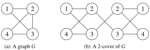
Figure 4: An example of a graph cover. Nodes in the cover are labeled by the node that they are a copy of inG.

Definition 8 A graph H coversa graph G if there exists a graph homomorphismπ:H_→G such thatπis an isomorphism on neighborhoods (i.e., for all vertices i_∈H,∂i is mapped bijectively onto ∂π(i)). Ifπ(i) =j, then we say that i_∈H is a copy of j_∈G. Further, H is an M-cover of G if every vertex of G has exactly M copies in H.

Graph covers, in the context of graphical models, were originally studied in relation to local message-passing algorithms for coding problems (Vontobel and Koetter, 2005). Graph covers may be connected (i.e., there is a path between every pair of vertices) or disconnected. However, when a graph cover is disconnected, all of the connected components of the cover must themselves be covers of the original graph. For a simple example of a connected graph cover, see Figure 4.

Every finite cover of a connected graph is anM-cover for some integerM. For every base graph

G, there exists a graph, possibly infinite, which covers all finite, connected covers of the base graph.

This graph is known as the universal cover.

To any finite cover, H, of a factor graphGwe can associate a collection of potentials derived

from the base graph; the potential at nodei∈His equal to the potential at nodeπ(i)_∈G. Together,

these potential functions define a new objective function for the factor graphH. In the sequel, we

will use superscripts to specify that a particular object is over the factor graphH. For example, we

will denote the objective function corresponding to a factor graphH as fH_{, and we will write f}G

for the objective function f.

Local message-passing algorithms such as the reweighted min-sum algorithm are incapable of

distinguishing the two factor graphsHandGgiven that the initial messages to and from each node

inHare identical to the nodes that they cover inG: for every nodei_∈Gthe messages received and

sent by this node at timet are exactly the same as the messages sent and received at timet by any

copy ofiinH. As a result, if we use a local message-passing algorithm to deduce an assignment

fori, then the algorithm run on the graphHmust deduce the same assignment for each copy ofi.

Now, consider an objective function f that factors over the graphG. For any finite coverHof

Gwith covering homomorphismπ:H_→G, we can “lift” any vector of beliefs,τG_{, fromGtoHby}

defining a new vector of beliefs,τH_{, such that:}

• For all variable nodesi_∈H,τH

i =τGπ(i).

• For all edges(i,j)_∈H,τH

i j =τGπ(i)π(j).

Analogously, we can lift any assignmentxG_{to an assignmentx}H _{by settingx}H

3.1 Graph Covers and Quadratic Minimization

LetGbe the pairwise factor graph for the objective function fG(x1, ...,xn) = 1₂xTΓx−hTxwhose

edges correspond to the nonzero entries ofΓ. LetHbe anM-cover ofGwith corresponding

objec-tive function fH(x11, ...,x1M, ...xnM) =1₂xTeΓx−ehTx. Without loss of generality we can assume that

e

Γandehtake the following form:

e

Γ =

  

Γ11P11 ··· Γ1nP1n

..

. . .. ...

Γn1Pn1 ··· ΓnnPnn

  ,

e

hi = h⌈i/M⌉, (1)

wherePi j=PTji is anM×Mpermutation matrix for alli6=jandPiiis theM×Midentity matrix for

alli. IfΓeis derived fromΓin this way, then we will say thateΓcoversΓ.

For the quadratic minimization problem, factor graphs and their covers share many of the same properties. Most notably, we can transform critical points of covers to critical points of the original

problem. Let H andG be as above, and let π be the graph homomorphism from H to G. For

x_∈R|VG|_{, define lift}

H:R|VG|→R|VH|such that

liftH(x)i=xπ(i)

for alli_∈H. Similarly, for eachy_∈R|VH|_{, define proj}

GR|VG|→R|VG|such that

proj(y)i=

∑

k∈H:π(k)=i

yk

|{j_∈H:π(j) =i_}|

for alli∈G. With these definitions, we have the following lemma.

Lemma 9 IfeΓy=eh for y_∈R|VH|_{, then Γ·proj}

G(y) =h. Conversely, ifΓx=h for y∈R|VG|, then

e

Γ_·lift_H(x) =eh.

Notice that these solutions correspond to critical points of the cover and the original problem. Similarly, we can transform eigenvectors of covers to either eigenvectors of the original problem or the zero vector.

Lemma 10 Fixλ_∈R. IfΓey=λy, then eitherΓ_·proj_G(y) =λproj_G(y)orΓ_·proj_G(y) =0. Con-versely, ifΓx=λx, theneΓ_·lift_H(x) =λlift_H(x).

These lemmas demonstrate that we can average critical points and eigenvectors of covers to obtain critical points and eigenvectors (or the zero vector) of the original problem, and we can lift critical points and eigenvectors of the original problem in order to obtain critical points and eigenvectors of covers.

Unfortunately, even though the critical points ofGand its covers must correspond via Lemma 9,

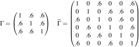
Γ=

 

1 .6 .6

.6 1 .6 .6 .6 1

  eΓ=

       

1 0 .6 0 0 .6

0 1 0 .6 .6 0

.6 0 1 0 .6 0

0 .6 0 1 0 .6

0 .6 .6 0 1 0

.6 0 0 .6 0 1

       

Figure 5: An example of a positive definite matrix,Γ, which possesses a 2-cover,eΓ, that has

nega-tive eigenvalues.

points of the reweighted algorithm on any graph cover. As such, the reweighted algorithm may not

converge to the correct minimizing assignment when the matrix corresponding to some cover ofG

is not positive definite. Consequently, we will first consider the special case in whichΓand all of its

covers are positive definite. We can exactly characterize the matrices for which this property holds.

Theorem 11 LetΓbe a symmetric matrix with positive diagonal. The following are equivalent.

1. Γis walk-summable.

2. Γis scaled diagonally dominant.

3. All covers ofΓare positive definite.

4. All 2-covers ofΓare positive definite.

Proof The two non-trivial implications in the proof (4_⇒1 and 1_⇒2) make use of the Perron-Frobenius theorem. For the complete details, see Appendix A.

This theorem has several important consequences. First, it provides us with a combinatorial char-acterization of scaled diagonal dominance and walk-summability. Second, it provides an intuitive explanation for why these conditions should be sufficient for the convergence of local message-passing algorithms.

More importantly, we can use Theorem 11 to conclude that MPLP, tree-reweighted max-product, and other message-passing algorithms that guarantee the correctness of locally decodable beliefs

cannot converge to the correct solution whenΓis positive definite but not walk-summable. From

the discussion in Section 3, every collection of locally decodable beliefs on the base graph can be lifted to locally decodable beliefs on any graph cover. Each of these “convergent and correct”

message-passing algorithms guarantees that the lift ofx∗to each graph cover must be a global

min-imum on that cover. By Theorem 11, there exists at least one graph cover with no global minmin-imum. As a result, these algorithms cannot converge to locally decodable beliefs.

As we saw in Theorem 5, the reweighted message-passing algorithm only guarantees thatx∗is

a local optimum. However, there exist simple choices for the reweighting parameters that guarantee correctness over all covers. As an example, ifci j ≤_maxi1

∈V|∂i| for all(i,j)∈E, then one can show

that the reweighted algorithm cannot converge to locally decodable beliefs unless all of the graph

corresponds to an edge appearance probability provides another example. Given this observation, in order to produce convergent message-passing schemes for the quadratic minimization problem, we will need to study choices of the parameters that do not guarantee correctness over all graph covers.

4. Convergence Properties of Reweighted Message-Passing Algorithms

Recall that the GaBP algorithm can converge to the correct minimizer of the objective function even if the original matrix is not scaled diagonally dominant. The most significant problem when the original matrix is positive definite but not scaled diagonally dominant is that the computation trees may eventually possess negative eigenvalues due to the existence of some 2-cover with at least one non-positive eigenvalue. If this happens, then some of the beliefs will not be bounded from below, and the corresponding estimate will be negative infinity. This is, of course, the correct answer on some 2-cover of the problem, but it is not the correct solution to the minimization problem of interest. Our goal in this section is to understand how the choice of the parameters and alternative message-passing orders affect the convergence of the reweighted algorithm.

4.1 Convergence of the Variances

First, we will provide conditions on the choice of the parameter vector such that all of the com-putation trees produced by the reweighted algorithm remain positive definite throughout the course of the algorithm. Positive definiteness of the computation trees corresponds to the convexity of the beliefs, and the convexity of the belief,τt

i, is determined only by the vectorat. As such, we begin

by studying the sequencea0,a1, ...wherea0is the zero vector (based on our initialization). We will

consider two different choices for the parameter vector: one in whichci j≥1 for alliand jand one

in whichci j<0 for alliand j. The latter of these two requires all of the parameters to be negative.

Such a choice is unusual among reweighted algorithms, but it does guarantee that the computation trees will remain positive definite throughout the algorithm. This observation and the experimental results in Section 4.4 suggest that such a choice might be worth studying in other contexts as well.

4.1.1 POSITIVEPARAMETERS

Lemma 12 If ci j≥1for all i and j, then for all t >0, ati→j≤ati→−1j≤0for each i and j.

Proof This result follows by induction ont. First, suppose thatci j ≥1. If the update is not valid,

thenat_i→j=₋∞which trivially satisfies the inequality. Otherwise, we have

at_i→j = −

_Γ

i j

ci j

2

Γii+∑k∈∂i\jckiat_k−_→1_i+ (cji−1)atj−→1i

≤

_Γ

i j

ci j

2

Γii+∑k_∈∂i_\jckiat_k−_→2_i+ (cji−1)at_j−_→2_i

= at_i−_→1_j,

where the inequality follows from the observation thatΓii+∑k_∈∂i_\jckia_kt−_→1_i+ (cji−1)atj−_→1i>0 and

   

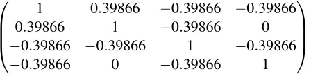
1 0.39866 ₋0.39866 ₋0.39866

0.39866 1 ₋0.39866 0

−0.39866 ₋0.39866 1 ₋0.39866

−0.39866 0 ₋0.39866 1

   

Figure 6: A positive definite matrix for which the variances in the min-sum algorithm converge but the means do not (Malioutov, 2008).

If we consider only the vectorat, then the algorithm may exhibit a weaker form of convergence.

Lemma 13 If ci j≥1for all i and j and all of the computation trees are positive definite, then the sequence a0_i→j,a1_i→j, ...converges.

Proof Suppose ci j ≥1. By Lemma 12, the ati→j are monotonically decreasing. Because all of

the computation trees are positive definite, we must have that for each i, Γii+∑k_∈∂i_\jckiat_k−_→1_i+ cjiatj−_→1i>0. Therefore, for all(i,j)∈E,ati_→j≥ −Γci jii. Consequently, the sequencea

0

i_→j,a1i→j, ...is

monotonically decreasing and bounded from below. This implies that the sequence converges.

Because the estimates of the variances only depend on the vectorat, if theat_i→j converge, then the estimates of the variances also converge. Therefore, requiring all of the computation trees to be positive definite is a sufficient condition for convergence of the variances. Note, however, that the

estimates of the means which correspond to the sequencebt_i→j need not converge even if all of the

computation trees are positive definite (see Figure 6).

Our strategy will be to ensure that all of the computation trees are positive definite by leveraging

the choice of parameters,ci j. Specifically, we want to use these parameters to weight the diagonal

elements of the computation tree much more than the off-diagonal elements in order to force the computation trees to be positive definite. If we can show that there is a choice of eachci j=cjithat

will cause all of the computation trees to be positive definite, then Algorithm 1 should behave almost as if the original matrix were scaled diagonally dominant. Indeed, there always exists a choice of the vectorcthat achieves this.

Theorem 14 For any symmetric matrixΓwith strictly positive diagonal,_∃r_≥1and anε>0such that the eigenvalues of the computation trees are bounded from below by ε when generated by Algorithm 1 with ci j=r for all i and j.

The proof of this theorem exploits the Gerˇsgorin disc theorem in order to show that there exists

a choice ofr such that each computation tree is scaled diagonally dominant. The complete proof

can be found in Appendix B.

4.1.2 NEGATIVEPARAMETERS

For the case in whichci j<0 for alliand j, we also have that the computation trees are always

posi-tive definite when the initial messages are uniformly equal to zero as characterized by the following lemmas.

Proof This result follows by induction ont. First, suppose thatci j <0 for all(i,j)∈E. If the

update is not valid, thenat_i→j=₋∞which trivially satisfies the inequality. Otherwise, we have

at_i→j = −

Γi j

ci j

2

Γii+∑k∈∂i\jckiatk−→1i+ (cji−1)atj−→1i

≤ 0,

where the inequality follows from the induction hypothesis.

Lemma 16 For any symmetric matrix Γwith strictly positive diagonal, if ci j <0 for all i and j, then all of the computation trees are positive definite.

Proof The computation trees are all positive definite if and only ifΓii+∑k∈∂ickiat_k→i>0 for allt.

By Lemma 15,at_i→j≤0 for allt, and as result,Γii+∑k∈∂ickiat_k→i≥Γii>0 for allt.

As when ci j ≥1 for all(i,j)∈E, the eigenvalues on each computation tree are again bounded

way from zero, but theat_i→j no longer form a monotonic decreasing sequence whenci j <0 for all

(i,j)_∈E. If all of the computation trees remain positive definite in the limit, then the beliefs will all be positive definite upon convergence. If the estimates for the means converge as well, then the converged beliefs must be locally decodable to the correct minimizing assignment. Notice that

none of the above arguments for the variances require Γto be positive definite. Indeed, we have

already seen an example of a matrix with a strictly positive diagonal and negative eigenvalues (see the matrix in Figure 5) such that the variance estimates converge.

4.2 Alternative Message Passing Schedules

The synchronous message-passing updates described in Algorithm 1 enforce a particular ordering on the updates performed at each time step. In practice, alternative message-passing schedules may improve the rate of convergence. One such alternative message-passing schedule is given by Algorithm 2. Because each computation tree produced by this algorithm is a principal submatrix of a synchronous computation tree and principal submatrices of positive definite matrices are positive definite, we can easily check that all of the results of the previous section extend to this modified schedule as well.

Algorithm 2 allows for quite a bit more flexibility in the scheduling of message updates, and as we will see experimentally in Section 4.4, it can have better convergence properties than the corresponding synchronous algorithm. To see why this might be the case, we will again exploit the properties of graph covers. Specifically, we will show that these two algorithms are related via a special 2-cover of the base factor graph.

Every pairwise factor graph,G= (VG,EG), admits a bipartite 2-cover,H= (VG× {1,2},EH),

called the Kronecker double cover ofG. We will denote copies of the variablexiin this 2-cover as

xi1 andxi2. For every edge(i,j)∈EG,(i1,j2)and(i2,j1)belong toEH. In this way, nodes labeled

with a one are only connected to nodes labeled with a two (see Figure 7). Note that ifGis already

a bipartite graph, then the Kronecker double cover ofGis simply two disjoint copies ofG.

Algorithm 2Alternative Reweighted Message-Passing Algorithm

1: Initialize the messages to some finite vector.

2: Choose some ordering of the variables such that each variable is updated infinitely often, and

perform the following update for each variable jin order

3: foreachi_∈∂jdo

4: Update the message fromito j:

mi→j(xj):=κ+min xi

h_{ψi j(xi,xj)}

ci j

+ (ci j−1)mj→i(xi) +φi(xi) +

∑

ckimk→i(xi)

i

.

5: end for

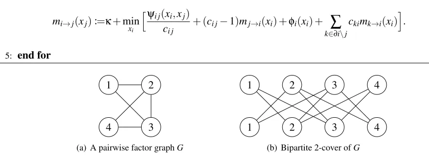
1 2

3 4

(a) A pairwise factor graphG

1 2 3 4

1 2 3 4

(b) Bipartite 2-cover ofG

Figure 7: The Kronecker double cover (b) of a pairwise factor graph (a). The node labeledi_∈G

corresponds to the variable nodexi.

Algorithm 3Bipartite Message-Passing Algorithm

1: Initialize the messages to some finite vector.

2: Iterate the following until convergence: update all of the outgoing messages from nodes labeled

one to nodes labeled two and then update all of the outgoing messages from nodes labeled two to nodes labeled one using the asynchronous update rule:

mi→j(xj):=κ+min xi

h_{ψi j(xi,xj)}

ci j

+ (ci j−1)mj→i(xi) +φi(xi) +

∑

ckimk→i(xi)

i

.

By construction, the message vector produced by Algorithm 3 is simply a concatenation of two

consecutive time steps of the synchronous algorithm. Specifically, for allt_≥1

mt_H=

m2_Gt−1 m2_Gt−2

.

Therefore, the messages passed by Algorithm 1 are identical to those passed by a specific or-dering of the updates in Algorithm 2 on the Kronecker double cover. From our earlier analysis, we

know that even ifΓis positive definite, not every cover necessarily corresponds to a convex

Algorithm 4Jacobi Iteration

1: Choose an initial vectorx0_∈Rn. 2: For iterationt=1,2, ...set

xt_j= hj−∑kΓjkx

t₋1

k

Γj j

for each j_{∈ {}1, ...,n_}.

Algorithm 5Gauss-Seidel Iteration 1: Choose an initial vectorx_∈Rn.

2: Choose some ordering of the variables, and perform the following update for each variable j,

in order,

xj=

hj−∑kΓjkxk

Γj j

.

4.2.1 THEGAUSS-SEIDEL ANDJACOBI METHODS

Because minimizing symmetric positive definite quadratic functions is equivalent to solving sym-metric positive definite linear systems, well-studied algorithms such as Gaussian elimination, Cholesky decomposition, etc. can be used to compute the minimum. In addition, many iterative algorithms

have been proposed to solve the linear systemΓx=h: Gauss-Seidel iteration, Jacobi iteration, the

algebraic reconstruction technique, etc.

In this section, we will show that the previous graph cover analysis can also be used to reason about the Jacobi and Gauss-Seidel algorithms (Algorithms 4 and 5). In Section 4.3, we will see that there is an even deeper connection between these algorithms and reweighted message-passing algorithms. WhenΓis symmetric positive definite, the objective function,1₂xT_Γx−hT_{x, is a convex}

function ofx. Consequently, we could use a coordinate descent scheme in an attempt to minimize

the objective function. The standard cyclic coordinate descent algorithm for this problem is known as the Gauss-Seidel algorithm.

In the same way that Algorithm 1 is a synchronous version of Algorithm 2, the Jacobi algorithm is a synchronous version of the Gauss-Seidel algorithm. To see this, observe that the iterates pro-duced by the Jacobi algorithm are related to the iterates of the Gauss-Seidel algorithm on a larger problem. Specifically, given a symmetricΓ_∈Rn×n_andh∈Rn_{, constructΓ}′_∈R2n×2n_andh′_∈R2n

as follows

h′_i =

h h

,

Γ′ =

D M

M D

,

whereDis a diagonal matrix with the same diagonal entries asΓandM=Γ₋D.

Γ′is the analog of the Kronecker double cover discussed in Section 4.2. Letx0_∈Rnbe an initial

vector for the Jacobi algorithm performed on the matrixΓand fix y0 _∈R2n such thaty0 =

x0 x0

.

Ifytis the vector produced aftertcomplete cycles of the Gauss-Seidel algorithm, thenyt =

x2t−1 x2t

.

Also, observe that, for anyyt such thatΓ′yt=h′, we must have thatΓhx2t−1+x2t

2

i

=h.

With these two observations, any convergence result for the Gauss-Seidel algorithm can be extended to the Jacobi algorithm.

Theorem 17 Let Γbe a symmetric positive semidefinite matrix with a strictly positive diagonal. The Gauss-Seidel algorithm converges to a vector x∗ such that Γx∗=h whenever such a vector exists.

Proof See Section 10.5.1 of Byrne (2008).

Using our observations, we can immediately produce the following new result.

Corollary 18 LetΓbe a symmetric positive semidefinite matrix with positive diagonal and letΓ′

be constructed as above. If Γ′ is a symmetric positive semidefinite matrix and there exists an x∗ such thatΓx∗=h, then the sequence xt+₂xt−1 converges to x∗where xt is the tthiterate of the Jacobi algorithm.

IfΓ′_{is not positive semidefinite, then the Gauss-Seidel algorithm (and by extension the Jacobi}

algorithm) may or may not converge when run onΓ′.

4.3 Convergence of the Means

If the variances converge, then the fixed points of the message updates for the means correspond to

the solution of a particular linear systemMb=d. In fact, we can show that Algorithm 2 is exactly

the Gauss-Seidel algorithm for this linear system. First, we construct the matrixM_∈R2|E|×2|E|:

Mi j,i j = A∗i\j for alli∈V and j∈∂i,

Mi j,ki = cki

Γi j ci j

for alli_∈V and for all j,k_∈∂isuch thatk₆= j,

Mi j,ji = (ci j−1)

Γi j ci j

for alli_∈V and j_∈∂i.

Here,A∗is constructed from the vector of converged variances,a∗. All other entries of the matrix

are equal to zero. Next, we define the vectord_∈R2|E| by settingdi j =hiΓi j/ci j for all i∈V and j_∈∂i.

By definition, any fixed point, b∗, of the message update equations for the means must satisfy

Mb∗=d. With these definitions, Algorithm 2 is precisely the Gauss-Seidel algorithm for this matrix.

Similarly, Algorithm 1 corresponds to the Jacobi algorithm. Unfortunately,Mis neither symmetric

0 5 10 15 20 0

0.2 0.4 0.6 0.8 1 1.2

Iterations

E

rr

o

r

Min-Sum Sync. Alg. 2

(a) p=.3

0 10 20 30

0 1 2 3 4 5

Iterations

E

rr

o

r

Min-Sum Sync. Alg. 2

(b) p=.398

0 10 20 30

0 1 2 3 4 5

Iterations

E

rr

or

Min-Sum Sync. Alg. 2

(c) p=.4

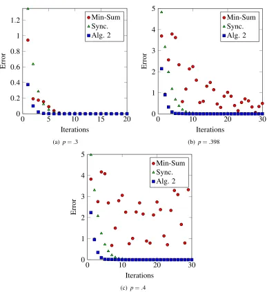
Figure 8: The error, measured by the 2-norm, between the current mean estimate and the true mean at each step of the min-sum algorithm, the alternative message-passing schedule in Algo-rithm 2 withci j=2 for alli6= j, and the synchronous algorithm withci j=2 for alli6= j

for the matrix in (2). Notice that all of the algorithms have a similar performance when

pis chosen such that the matrix is scaled diagonally dominant. When the matrix is not

scaled diagonally dominant, the min-sum algorithm converges more slowly or does not converge at all.

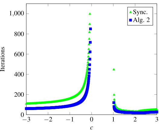
4.4 Experimental Results

Even simple experiments demonstrate the advantages of the reweighted message-passing algorithm

−3 ₋2 ₋1 0 1 2 3 0

200 400 600 800 1,000

c

Ite

ra

tio

n

s

Sync. Alg. 2

Figure 9: The number of iterations needed to reduce the error of the mean estimates below 10−6

using the reweighted algorithms as a function ofcfor the matrix in (2) withp=.4. The

gap in the plot is predicted by the arguments at the end of Section 3.1.

chosen to be the vector of all ones. LetΓbe the following matrix.

   

1 p ₋p ₋p

p 1 ₋p 0

−p ₋p 1 ₋p −p 0 ₋p 1

  

. (2)

The standard min-sum algorithm converges to the correct solution for 0_≤p< .39865 (Malioutov

et al., 2006). Figure 8 illustrates the behavior of the min-sum algorithm, Algorithm 2 withci j=2

for alli6= j, and the synchronous algorithm withci j =2 for alli6= jfor different choices of the

constant p. Each iteration of Algorithm 2 algorithm consists of cyclically updating the incoming

messages to all nodes. In the examples in Figure 8, the synchronous algorithm and Algorithm 2 always converge rapidly to the correct mean while the min-sum algorithm converges slowly or not at all aspapproaches.5.

While this is a simple graph, the behavior of the algorithm for different choices of the vectorc

is already apparent. If we setci j=3 for alli6= j, then empirically, both the synchronous algorithm

and Algorithm 2 converge for all p∈(₋.5, .5), the entire positive definite region for this matrix.

However, different choices of the parameter vector can greatly increase or decrease the number of iterations required for convergence. Figure 9 illustrates the iterations to convergence for the

reweighted algorithms at p=.4 versusc.

−4 ₋2 0 2 4 0

500 1,000 1,500 2,000

c

Ite

ra

tio

n

s

Sync. Alg. 2

Figure 10: The number of iterations needed to reduce the error of the mean estimates below 10−6

using the reweighted algorithms as a function ofcfor the matrix in (3). Again, the gap

in the plot is predicted by the arguments at the end of Section 3.1.

for sufficiently largec. Figure 10 illustrates these convergence issues for the matrix,

   

45 21 23 ₋42

21 83 8 ₋32

23 8 14 ₋29

−42 ₋32 ₋29 134

  

. (3)

The above matrix was randomly generated. Similar observations can be made for many other posi-tive definite matrices as well.

5. Conclusions and Future Research

5.1 Convergence

The main open questions surrounding the performance of the reweighted algorithm relate to

ques-tions of convergence. First, for all positive definiteΓ, we conjecture that there exists a sufficiently

large (or sufficiently negative) choice of the parameters such that the means always converge under Algorithm 2.

Second, in practice, one typically uses a damped version of the message updates in order to attempt to force convergence. For the min-sum algorithm, the damped updates are given by

mt_i→j(xj) = κ+δmti→j(xj) + (1−δ)

h

min

xi

ψi j(xi,xj) +φi(xi) +

∑

mt_k−_→1_i(xi)

i

for some δ_∈[0,1). The damped min-sum algorithm with damping factor δ=1/2 empirically

seems to converge ifΓis positive definite and all of the computation trees remain positive definite

(Malioutov et al., 2006). We make the same observation for the damped version of Algorithm 1.

In practice, the damped synchronous algorithm withδ=1/2 and Algorithm 2 appear to

con-verge for all sufficiently large choices of the parameter vector as long asΓis positive definite. We

conjecture that this is indeed the case: for all positive definiteΓthere exists acsuch that ifci j=cfor

alli₆= j, then the damped algorithm and Algorithm 2 always converge. In this line of exploration,

the relationship between the synchronous algorithm and Algorithm 2 described in Section 4.2 may be helpful.

Finally, Moallemi and Van Roy (2010) were able to provide rates of convergence in the case

thatΓis walk-summable by using a careful analysis of the computation trees. Perhaps similar ideas

could be adapted for the computation trees produced by the reweigthed algorithm.

5.2 General Convex Minimization

The reweighted algorithm can, in theory, be applied to minimize general convex functions, but in practice, computing and storing the message vector for these more general models may be inef-ficient. Despite this, many of the previous observations can be extended to the general case of a

convex function f :C→Rsuch thatC⊆Rnis a convex set.

As was the case for quadratic minimization, convexity of the objective function fG does not

necessarily guarantee convexity of the objective function fH for every finite coverH ofG. Recall

that the existence of graph covers that are not bounded from below can be problematic for the reweighted message-passing algorithm. For quadratic functions, this cannot occur if the matrix is scaled diagonally dominant or, equivalently, if the objective function corresponding to every finite graph cover is positive definite. This equivalence suggests a generalization of scaled diagonal dominance for arbitrary convex functions based on the convexity of their graph covers. Such convex functions would have desirable properties with respect to iterative message-passing schemes.

Lemma 19 Let f be a convex function that factorizes over a graph G. Suppose that for every finite cover H of G, fH is convex. If xG_∈arg minx f(x), then for every finite cover H of G, xH, the lift of xGto H, minimizes fH.

Proof This follows from the observation that all convex functions are subdifferentiable over their

domains and thatxHis a minimum of fHif and only if the zero vector is contained in the subgradient

Even if the objective function is not convex for some cover, we may still be able to use the same trick

as in Theorem 14 in order to force the computation trees to be convex. LetC_⊆Rnbe a convex set. If

f :C_→Ris twice continuously differentiable, then fis convex if and only if its Hessian, the matrix

of second partial derivatives, is positive semidefinite on the interior ofC. For each fixedx∈C,

Theorem 14 demonstrates that there exists a choice of the vectorcsuch that all of the computation

trees are convex atx, but it does not guarantee the existence of acthat is independent ofx.

For twice continuously differentiable functions, Moallemi and Van Roy (2010) provide suffi-cient conditions for the convergence of the min-sum algorithm that are based on a generalization of scaled diagonal dominance, and extending the above ideas is the subject of future research.

Appendix A. Proof of Theorem 11

Without loss of generality, we can assume thatΓhas a unit diagonal. We break the proof into several

pieces:

• (1_⇒2) Without loss of generality we can assume that _|I₋Γ_|is irreducible (if not we can

make this argument on each of its connected components). Let 1>λ>0 be an eigenvalue

of _|I₋Γ_| with eigenvector x>0 whose existence is guaranteed by the Perron-Frobenius

theorem. For any rowi, we have:

xi>λxi=

∑

|Γi j|xj.

SinceΓii=1 this is the definition of scaled diagonal dominance withw=x.

• (2_⇒3) If Γ is scaled diagonally dominant then so is every one of its covers. Scaled

di-agonal dominance of a symmetric matrix with a positive didi-agonal implies that the matrix is symmetric positive definite. Therefore, all covers must be symmetric positive definite.

• (3_⇒4)Trivial.

• (4_⇒1)LetΓebe any 2-cover ofΓ. Without loss of generality, we can assume thateΓhas the

form (1).

First, observe that by the Perron-Frobenius theorem there exists an eigenvectorx>0_∈Rnof

|I−Γ_|with eigenvalueρ(_|I−Γ_|). Lety∈R2nbe constructed by duplicating the values ofx so thaty2i=y2i+1=xifor eachi∈ {0...n}. By Lemma 10,yis an eigenvector of|I−Γe|with

eigenvalue equal toρ(_|I₋Γ_|). We claim that this implies ρ(_|I₋eΓ_|) =ρ(_|I₋Γ_|). Assume without loss of generality that_|I−Γe_|is irreducible; if not, then we can apply the following

argument to each connected component of_|I₋eΓ_|. By the Perron-Frobenius theorem again,

|I₋Γe_|has a unique positive eigenvector (up to scalar multiple), with eigenvalue equal to the spectral radius. Thus,ρ(_|I₋Γ_|) =ρ(_|I₋Γe_|)becausey>0.

We will now construct a specific cover eΓsuch thateΓis positive definite if and only ifΓis

walk-summable. To do this, we’ll choose thePi j as in (1) such that Pi j =I if Γi j <0 and

Pi j =

0 1

1 0

otherwise. Now definez_∈R2n by settingzi= (−1)icyi, where the constantc

Consider the following:

zTeΓz =

n

∑

∑

Γi j[z2i,z2i+1]Pi j

z2j z2j+1

+

_∑

i

Γiiz2i

= 1₋2

∑

i>j

|Γi j|c2yiyj.

Recall thatyis the eigenvector of_|I₋eΓ_|corresponding to the largest eigenvalue and_kcy_k=1. By definition and the above,

ρ(_|I₋Γ_|) = ρ(_|I₋Γe_|)

= cy

T_|I−Γe|cy c2_yT_y

= 2

∑

i>j

|Γi j|c2yiyj.

Combining all of the above we see thatzTΓez=1₋ρ(_|I₋Γ_|). Now,Γepositive definite implies thatzT_{eΓz>0, so 1−ρ(|I−Γ|)>0. In other words,Γis walk-summable.}

Appendix B. Proof of Theorem 14

Let Tv(t) be the deptht computation tree rooted at v, and let Γ′ be the matrix corresponding to

Tv(t)(i.e., the matrix generated by the potentials in the computation tree). We will show that the

eigenvalues ofΓ′are bounded from below by someε>0. For anyi_∈Tv(t)at depthddefine:

wi =

_s

r

d

,

whereris as in the statement of the theorem andsis a positive real to be determined below. LetW

be a diagonal matrix whose entries are given by the vectorw. By the Gerˇsgorin disc theorem (Horn

and Johnson, 1990), all of the eigenvalues ofW−1Γ′W are contained in

∪i∈Tv(t)

n

z_∈R:_|z₋Γ′_{ii| ≤} 1 wi

∑

wj|Γ′i j|

o

.

Because all of the eigenvalues are contained in these discs, we need to show that there is a choice ofsandrsuch that for alli_∈Tv(t),|Γ′ii| −w1i∑j6=iwj|Γ

′

i j| ≥ε.

Recall from Section 2.2.1 that_|Γ′_{i j|}=η|Γi j|

r for some constantηthat depends onr. Further, all

potentials below the potential on the edge(i,j)are multiplied byηγfor some constantγ. We can

divide out by this common constant to obtain equations that depend onr and the elements of Γ.

Note that some self-potentials will be multiplied byr₋1 while others will be multiplied byr. With

this rewriting, there are three possibilities:

1. iis a leaf ofTv(t). In this case, we need|Γii|> _w1_i| Γip(i)|

r wp(i). Plugging in the definition ofwi,

we have

|Γii|>|

Γip(i)|

2. iis not a leaf ofTv(t)or the root. In this case, we need

|Γii| >

1 wi

h_|Γip(i)|

r wp(i)+

s2(r₋1)

r3 |Γip(i)|wp(i)+

∑

k∈∂i−p(i)

|Γki|wk

i

.

Again, plugging the definition ofwiinto the above yields

|Γ′_ii| > |Γip(i)|

s +

s r

h_r−1

r |Γip(i)|+_k

∑

∈∂i−p(i)

|Γki|

i

.

3. iis the root ofTv(t). Similar to the previous case, we need |Γii|wi>∑k∈∂i|Γki|wk. Again,

plugging the definition ofwiinto the above yields

|Γii|> s

r_k

∑

None of these bounds are time dependent. As such, if we choose sandr to satisfy the above

constraints, then there must exist someε>0 such that smallest eigenvalue of any computation tree

is at leastε. Fixsto satisfy (4) for all leaves ofTv(t). This implies that(|Γii| −| Γip(i)|

s )>0 for any i∈Tv(t). Finally, we can choose a sufficiently largerthat satisfies the remaining two cases for all i_∈Tv(t).

References

C. L. Byrne. Applied Iterative Methods. A K Peters, Ltd., 2008.

B. J. Frey, R. Koetter, and A. Vardy. Signal-space characterization of iterative decoding.Information

Theory, IEEE Transactions on, 47(2):766–781, Feb. 2001.

A. Globerson and T. S. Jaakkola. Fixing max-product: Convergent message passing algorithms for

MAP LP-relaxations. InProc. Neural Information Processing Systems (NIPS), Vancouver, B. C.,

Canada, Dec. 2007.

T. Hazan and A. Shashua. Norm-product belief propagation: Primal-dual message-passing for

approximate inference. Information Theory, IEEE Transactions on, 56(12):6294 –6316, Dec.

2010.

R. A. Horn and C. R. Johnson. Matrix Analysis. Cambridge University Press, 1990.

J. K. Johnson, D. Bickson, and D. Dolev. Fixing convergence of Gaussian belief propagation. In Proc. Information Theory, IEEE International Symposium on (ISIT), pages 1674–1678, Seoul, South Korea, July 2009.

D. M. Malioutov. Approximate inference in Gaussian graphical models. Ph.D. thesis, EECS, MIT, 2008.

D. M. Malioutov, J. K. Johnson, and A. S. Willsky. Walk-sums and belief propagation in Gaussian

T. Meltzer, A. Globerson, and Y. Weiss. Convergent message passing algorithms: a unifying view. InProc. of the 25th Conference on Uncertainty in Artificial Intelligence (UAI), Montreal, Canada, June 2009.

C. C. Moallemi and B. Van Roy. Convergence of min-sum message passing for quadratic

optimiza-tion. Information Theory, IEEE Transactions on, 55(5):2413 –2423, May 2009.

C. C. Moallemi and B. Van Roy. Convergence of min-sum message-passing for convex optimization. Information Theory, IEEE Transactions on, 56(4):2041 –2050, April 2010.

N. Ruozzi, J. Thaler, and S. Tatikonda. Graph covers and quadratic minimization. InProc.

Com-munication, Control, and Computing, 47th Annual Allerton Conference on, Allerton, IL, Sept. 2009.

D. Sontag and T. S. Jaakkola. Tree block coordinate descent for MAP in graphical models. In

Pro-ceedings of the 12th International Conference on Artificial Intelligence and Statistics (AISTATS), Clearwater Beach, Florida, April 2009.

S. Tatikonda and M. I. Jordan. Loopy belief propagation and Gibbs measures. In Proc. of the

Conference on Uncertainty in Artificial Intelligence (UAI), pages 493–500, Edmonton, Alberta, Canada, 2002.

P. O. Vontobel and R. Koetter. Graph-cover decoding and finite-length analysis of message-passing

iterative decoding of LDPC codes. CoRR, abs/cs/0512078, 2005.

M. J. Wainwright, T. S. Jaakkola, and A. S. Willsky. Tree-based reparameterization framework for

analysis of sum-product and related algorithms. Information Theory, IEEE Transactions on, 49

(5):1120 – 1146, May 2003a.

M. J. Wainwright, T. S. Jaakkola, and A. S. Willsky. Tree-reweighted belief propagation algorithms

and approximate ML estimation via pseudo-moment matching. InProceedings of the 9th

Inter-national Conference on Artificial Intelligence and Statistics (AISTATS), Key West, Florida, Jan. 2003b.

M. J. Wainwright, T. S. Jaakkola, and A. S. Willsky. Tree consistency and bounds on the

perfor-mance of the max-product algorithm and its generalizations. Statistics and Computing, 14(2):

143–166, 2004.

M. J. Wainwright, T. S. Jaakkola, and A. S. Willsky. MAP estimation via agreement on (hyper)trees:

message-passing and linear programming. Information Theory, IEEE Transactions on, 51(11):

3697–3717, Nov. 2005.

Y. Weiss. Correctness of local probability propagation in graphical models with loops. Neural

Comput., 12(1):1–41, 2000.

Y. Weiss and W. T. Freeman. On the optimality of solutions of the max-product belief-propagation

algorithm in arbitrary graphs. Information Theory, IEEE Transactions on, 47(2):736 –744, Feb.

Y. Weiss and W. T. Freeman. Correctness of belief propagation in Gaussian graphical models of

arbitrary topology. Neural Comput., 13(10):2173–2200, Oct. 2001b.

T. Werner. A linear programming approach to max-sum problem: A review. Pattern Analysis and