Minimax Manifold Estimation

Minimax Manifold Estimation

Christopher R. Genovese [email protected]

Department of Statistics Carnegie Mellon University 5000 Forbes Ave.

Pittsburgh, PA 15213, USA

Marco Perone-Pacifico [email protected]

Dipartimento di Scienze Statistiche Sapienza University of Rome

Piazzale Aldo Moro 5 – 00185 Roma, Italy

Isabella Verdinelli∗ [email protected]

Larry Wasserman† [email protected]

Department of Statistics Carnegie Mellon University 5000 Forbes Ave.

Pittsburgh, PA 15213, USA

Editor: Ulrike von Luxburg

Abstract

We find the minimax rate of convergence in Hausdorff distance for estimating a manifold M of dimension d embedded inRD_{given a noisy sample from the manifold. Under certain conditions,} we show that the optimal rate of convergence is n−2/(2+d). Thus, the minimax rate depends only on the dimension of the manifold, not on the dimension of the space in which M is embedded. Keywords: manifold learning, minimax estimation

1. Introduction

We consider the problem of estimating a manifold M given noisy observations near the manifold. The observed data are a random sample Y1, . . . ,Ynwhere Yi∈RD. The model for the data is

Yi=ξi+Zi

where ξ1, . . . ,ξn are unobserved variables drawn from a distribution supported on a manifold M

with dimension d<D. The noise variables Z1, . . . ,Znare drawn from a distribution F. Our main

assumption is that M is a compact, d-dimensional, smooth Riemannian submanifold in RD_{; the}

precise conditions on M are given in Section 2.1.

A manifold M and a distribution for(ξ,Z)induce a distribution Q_≡QM for Y . In Section 2.2,

we define a class of such distributions

Q

=nQM: M∈

M

o

where

M

is a set of manifolds. Given two sets A and B, the Hausdorff distance between A and B is

H(A,B) =inf

n

ε: A_⊂B_⊕ε and B_⊂A_⊕ε

o

where

A⊕ε=[

x∈A

BD(x,ε)

and BD(x,ε)is an open ball inRDcentered at x with radiusε. We are interested in the minimax risk

Rn(

Q

) =inf

b

M

sup

Q∈Q

E_Q[H(Mb_,M)]

where the infimum is over all estimatorsM. By an estimatorb M we mean a measurable function ofb Y1, . . . ,Yn taking values in the set of all manifolds. Our first main result is the following minimax

lower bound which is proved in Section 3.

Theorem 1 Under assumptions (A1)-(A4) given in Section 2, there is a constant C1>0 such that,

for all large n,

inf b

M

sup

Q_∈Q

E_Qh_H(Mb_,M)i_≥C1

1

n

2

2+d

where the infimum is over all estimatorsM.b

Thus, no method of estimating M can have an expected Hausdorff distance smaller than the stated bound. Note that the rate depends on d but not on D even though the support of the distribution

Q for Y has dimension D. Our second result is the following upper bound which is proved in Section

4.2.

Theorem 2 Under assumptions (A1)-(A4) given in Section 2, there exists an estimatorM such that,b for all large n,

sup

Q∈Q

E_Qh_H(Mb_,M)i_≤C2

log n

n

2

2+d

for some C2>0.

Thus the rate is tight, up to logarithmic factors. The estimator in Theorem 2 is of theoretical interest because it establishes that the lower bound is tight. But, the estimator constructed in the proof of that theorem is not practical and so in Section 5, we construct a very simple estimatorMb

such that

sup

Q∈Q

E_Qh_H(Mb_,M)i_≤

C log n n

1/D

.

1.1 Related Work

There is a vast literature on manifold estimation. Much of the literature deals with using manifolds for the purpose of dimension reduction. See, for example, Baraniuk and Wakin (2007) and refer-ences therein. We are interested instead in actually estimating the manifold itself. There is a large literature on this problem in the field of computational geometry; see, for example, Dey (2006), Dey and Goswami (2004), Chazal and Lieutier (2008) Cheng and Dey (2005) and Boissonnat and Ghosh (2010). However, very few papers allow for noise in the statistical sense, by which we mean observations drawn randomly from a distribution. In the literature on computational geometry, ob-servations are called noisy if they depart from the underlying manifold in a very specific way: the observations have to be close to the manifold but not too close to each other. This notion of noise is quite different from random sampling from a distribution. An exception is Niyogi et al. (2008) who constructed the following estimator. Let I=_{i : pb(Yi)>λ}where bp is a density estimator. They

defineMb=S_i∈IBD(Yi,ε)and they show that ifλandεare chosen properly, thenM is homologousb

to M. (This means that M andM share certain topological properties.) However, the result does notb

guarantee closeness in Hausdorff distance. Note thatSn_i=1BD(Yi,ε) is precisely the Devroye-Wise

estimator for the support of a distribution (Devroye and Wise, 1980).

1.2 Notation

Given a set S, we denote its boundary by∂S. We let BD(x,r) denote a D-dimensional open ball

centered at x with radius r. If A is a set and x is a point then we write d(x,A) =infy∈A||x−y||where || · ||is the Euclidean norm. Let

A_◦B= (A_∩Bc)[(Ac_∩B)

denote symmetric set difference between sets A and B.

The uniform measure on a manifold M is denoted by µM. Lebesgue measure onRk is denoted

byνk. In case k=D, we sometimes write V instead ofνD; in other words V(A)is simply the volume

of A. Any integral of the formR f is understood to be the integral with respect to Lebesgue measure

onRD_{. If P and Q are two probability measures onR}D_{with densities p and q then the Hellinger}

distance between P and Q is

h(P,Q)_≡h(p,q) =

r_Z

(√p₋√q)2₌

s

2

1₋

Z _√

pq

where the integrals are with respect toνD. Recall that

ℓ1(p,q)≤h(p,q)≤

p

ℓ1(p,q) (1)

whereℓ1(p,q) =R|p−q|. Let p(x)∧q(x) =min{p(x),q(x)}. The affinity between P and Q is ||P_∧Q_||=

Z

p_∧q=1₋1 2 Z

|p₋q_|.

Let Pn denote the n-fold product measure based on n independent observations from P. In the appendix Section 7.1 we show that

||Pn_∧Qn_{|| ≥} 1

2

1₋1 2 Z

|p₋q_|

2n

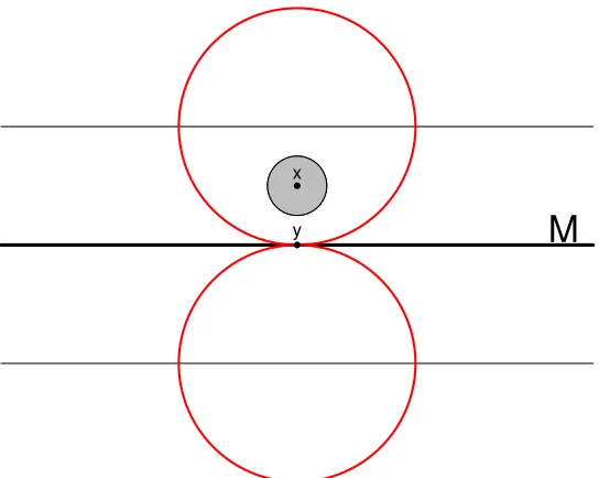
Figure 1: The condition number∆(M)of a manifold is the largest numberκsuch that the normals to the manifold do not cross as long as they are not extended beyondκ. The plot on the left shows a one-dimensional manifold (a curve) and some normals of length r<κ. The plot on the right shows the same manifold and some normals of length r>κ.

We write Xn=OP(an)to mean that, for everyε>0 there exists C>0 such thatP(||Xn||/an>C)≤ε

for all large n. Throughout, we use symbols like C,C0,C1,c,c0,c1. . . to denote generic positive

constants whose value may be different in different expressions.

2. Model Assumptions

In this section we describe all the assumptions on the manifold and on the underlying distributions.

2.1 Manifold Conditions

We shall be concerned with d-dimensional compact Riemannian submanifolds without boundary embedded inRD_{with d<D. (Informally, this means that M looks likeR}d _{in a small neighborhood}

around any point in M.) We assume that M is contained in some compact set

K

_⊂RD_.

At each u∈M let TuM denote the tangent space to M and let Tu⊥M be the normal space. We

can regard TuM as a d-dimensional hyperplane inRDand we can regard Tu⊥M as the D−d

dimen-sional hyperplane perpendicular to TuM. Define the fiber of size a at u to be La(u)≡La(u,M) =

T_u⊥MTBD(u,a).

Let∆(M)be the largest r such that each point in M_⊕r has a unique projection onto M. The

quantity∆(M)will be small if either M highly curved or if M is close to being self-intersecting. Let

M

≡

M

(κ)denote all d-dimensional manifolds embedded in

K

such that∆(M)_≥κ. Throughout this paper,κis a fixed positive constant. The quantity∆(M)has been rediscovered many times. It is called the condition number in Niyogi et al. (2006), the thickness in Gonzalez and Maddocks (1999) and the reach in Federer (1959).

An equivalent definition of∆(M) is the following: ∆(M)is the largest number r such that the fibers Lr(u)never intersect. See Figure 1. Note that if M is a sphere then∆(M)is just the radius of

the sphere and if M is a linear space then∆(M) =∞. Also, ifσ<∆(M)then M_⊕σis the disjoint union of its fibers:

M⊕σ= [

u∈M

Lσ(u). (3)

Let p,q∈M. The angle between two tangent spaces Tpand Tqis defined to be

angle(Tp,Tq) =cos−1

min

u∈Tp max

v_∈Tq|h

u₋p,v₋q_i|

wherehu,vi is the usual inner product inRD_{. Let d}

M(p,q) denote the geodesic distance between

p,q_∈M.

We now summarize some useful results from Niyogi et al. (2006).

Lemma 3 Let M_⊂

K

be a manifold and suppose that∆(M) =κ>0. Let p,q_∈M.

1. Letγbe a geodesic connecting p and q with unit speed parameterization. Then the curvature ofγis bounded above by 1/κ.

2. cos(angle(Tp,Tq))>1−dM(p,q)/κ. Thus,angle(Tp,Tq)≤

p

2dM(p,q)/κ+o(

p

dM(p,q)/κ).

3. If a=_||p₋q_{|| ≤}κ/2 then dM(p,q)≤κ−κ

p

1₋(2a)/κ=a+o(a).

4. If a=_||p₋q_{|| ≤}κ/2 then a_≥dM(p,q)−(dM(p,q))2/(2κ).

5. If_||q₋p_||>εand v_∈BD(q,ε)∩Tp⊥M∩BD(p,κ)then||v−p||<ε2/κ.

6. Fix anyδ>0. There exists points x1, . . . ,xN∈M such that M⊂SNj=1BD(xj,δ)and such that

N≤(c/δ)d_.

For further information about manifolds, see Lee (2002).

2.2 Distributional Assumptions

The distribution of Y is induced by the distribution of ξand Z. We will assume that ξ is drawn uniformly on the manifold. Then we assume that Z is drawn uniformly on the normal to M. More precisely, givenξ, we draw Z uniformly on L_σ(ξ). In other words, the noise is perpendicular to the manifold. The result is that, ifσ<κ, then the distribution Q=QMof Y has support equal to M⊕σ.

The distributional assumption onξis not critical. Any smooth density bounded away from 0 on the manifold will lead to similar results. However, the assumption on the noise Z is critical. We have chosen the simplest noise distribution here. (Perpendicular noise is also assumed in Niyogi et al., 2008.) In current work, we are deriving the rates for more complicated noise distributions. The rates are quite different and the proofs are more complex. Those results will be reported elsewhere. The set of distributions we consider is as follows. Letκandσbe fixed positive numbers such that 0<σ<κ. Let

Q

_≡

Q

(κ,σ) =nQM: M∈

M

(κ)

o

.

For any M_∈

M

(κ)consider the corresponding distribution QM, supported on SM=M⊕σ. Let

qMbe the density of QMwith respect to Lebesgue measure. We now show that qMis bounded above

and below by a uniform density.

Recall that the essential supremum and essential infimum of qM are defined by

ess sup

y∈A

qM=inf

n

and

ess inf

y_∈A qM=sup

n

a_∈R_: ν_{D({y : qM(y)<a} ∩A) =0}o_.

Also recall that, by the Lebesgue density theorem, qM(y) =limε→0QM(BD(y,ε))/V(BD(y,ε))for

almost all y. Let UMbe the uniform distribution on M⊕σand let uM=1/V(M⊕σ)be the density

of UM. Note that, for A⊂M⊕σ, UM(A) =V(A)/V(M⊕σ).

Lemma 4 There exist constants 0<C_∗≤C∗<∞, depending only onκand d, such that

C_∗≤ inf

M_∈Mess infy∈SM

qM(y)

uM(y) ≤

sup

M∈M

ess sup

y∈SM

qM(y)

uM(y) ≤

C∗.

Proof Choose any M∈

M

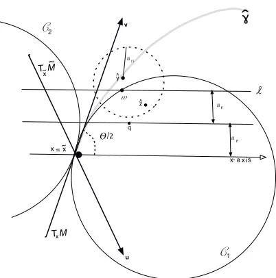
(κ). Let x by any point in the interior of SM. Let B=BD(x,ε)where ε>0 is small enough so that B_⊂SM=M⊕σ. Let y be the projection of x onto M. We want to

upper and lower bound Q(B)/V(B). Then we will take the limit asε_→0. Consider the two spheres of radiusκtangent to M at y in the direction of the line between x and y. (See Figure 2.) Note that

Q(B)is maximized by taking M to be equal to the upper sphere and Q(B)is minimized by taking M to be equal to the lower sphere. Let us consider first the case where M is equal to the upper sphere. Let

U=nu_∈M : L_σ(u)_∩B₆=/0o

be the projection of B onto M. By simple geometry, U =M_∩BD(y,rε)where

1+σ

κ

−1

≤r_≤1+σ

κ

.

Let Voldenote d-dimensional volume on M. Then Vol(BD(y,rε)∩M)≤c1rdεdωd where ωd is

the volume of a unit d-ball and c1 depends only on κ and d. To see this, note that because M

is a manifold and∆(M)_≥κ, it follows that near y, M may be locally parameterized as a smooth function f = (f1, . . . ,fD−d) over B∩TyM. The surface area of the graph of f over B∩TyM is

bounded by R_B

D(y,rε)∩TyM

q

1+_k∇fik2, which is bounded by a constant c1 uniformly over

M

.

Hence,Vol(BD(y,rε)∩M)≤c1Vol(BD(y,rε)∩TyM) =c1rdεdωd.

LetΛMbe the uniform distribution on M and letΓudenote the uniform measure on Lσ(u). Note

that, for u_∈U , Lσ(u)_∩B is a(D₋d)-ball whose radius is at mostε. Hence,

Γu(Lσ(u)∩B)≤ εD₋d_ω

D−d σD−dω

D−d

=ε

σ

D−d

.

Thus,

QM(B) =

Z

MΓu

(B_∩L_σ(u))dΛM(u) =

Z

UΓu

(B_∩L_σ(u))dΛM(u)

≤ _σεD−dΛ(U) =ε

σ

D−d_{Vol(BD(y,r)∩M)}

Vol(M)

≤ _σεD−d ε d_rd_ω

d

Vol(M) ≤

_ε

σ

D−dεd_(1+σ/κ)d_ω d

Figure 2: Figure for proof of Lemma 4. x is a point in the support M_⊕σ. y is the projection of x onto M. The two spheres are tangent to M at y and have radiusκ.

Now, UM(B) =V(B)/V(M⊕σ) =εDωD/(σD−dVol(M)). Hence,

QM(B)

UM(B) ≤

1+σ_κdωd.

Taking limits asε→0 we have that qM(y)≤C∗uM(y)for almost all y.

The proof of the lower bound is similar to the upper bound except for the following changes: let

U0denote all u∈U such that the radius of B∩Lσ(u)is at leastε/2. ThenΛ(U0)≥Λ(U)(1−O(ε))

and the projection of U0onto M is again of the form BD(y,rε)∩M. By Lemma 5.3 of Niyogi et al.

(2006),

Vol(BD(y,r)∩M)≥

1₋r

2_ε2

4κ2

d/2 rdεdωd

and the latter is larger than 2−d/2rdεdωd for all smallε. Also,Γu(Lσ(u)∩B)≥(ε/(2σ))D−dfor all

u_∈U0.

Of course, an immediate consequence of the above lemma is that, for every M ∈

M

(κ) and every measurable set A, C_∗UM(A)≤QM(A)≤C∗UM(A). We conclude this section by recording all

the assumptions in Theorems 1 and 2:

(A1) The manifold M is d-dimensional and is contained in a compact set

K

⊂RD_{with d<D.}

(A2) The manifold M satisfies∆(M)_≥κ>0.

(A3) The observed data Y1, . . . ,Yn are iid observations with Yi=Xi+ξi. Here,ξ1, . . . ,ξnare drawn

(A4) The noise levelσsatisfies 0<σ<κ.

Remark: As noted by a referee, the assumptions are very specific and the results do depend

criti-cally on the assumptions especially the assumption that d is known.

Remark: A referee has pointed out that another reasonable model is to assume that the Yi have a

uniform distribution on the tube of sizeσaround the manifold. To the best of our knowledge, this does not correspond to our model except in the special case where∆(M) =∞. However, all the results of our paper still apply in this case as long asσ<κ.

3. Minimax Lower Bound

In this section we derive a lower bound on the minimax rate of convergence for this problem. We will make use of the following result due to LeCam (1973). The following version is from Lemma 1 of Yu (1997).

Lemma 5 (Le Cam 1973) Let

Q

be a set of distributions. Letθ(Q)take values in a metric space with metricρ. Let Q0,Q1∈

Q

be any pair of distributions in

Q

. Let Y1, . . . ,Yn be drawn iid from

some Q_∈

Q

and denote the corresponding product measure by Qn. Letbθ(Y1, . . . ,Yn)be any

estima-tor. Then

sup

Q∈Q

E_Qn

h

ρ(bθ(Y1, . . . ,Yn),θ(Q))

i

≥ρ θ(Q0),θ(Q1)

||Qn_0∧Qn_1||.

To get a useful bound from Le Cam’s lemma, we need to construct an appropriate pair Q0and Q1. This is the topic of the next subsection.

3.1 A Geometric Construction

In this section, we construct a pair of manifolds M0,M1∈

M

(κ) and corresponding distributions Q0,Q1for use in Le Cam’s lemma. An informal description is as follows. Roughly speaking, M0

and M1 minimize the Hellinger distance h(Q0,Q1)subject to their Hausdorff distance H(M0,M1)

being equal to a given valueγ. Let

M0=

n

(u1, . . . ,ud,0, . . . ,0): −1≤uj≤1,1≤ j≤d

o

be a d-dimensional hyperplane inRD_{. Hence} ∆_(M

0) =∞. Place a hypersphere of radius κbelow M0. Push the sphere upwards into M0causing a bump of heightγat the origin. This creates a new

manifold M₀′ such that H(M0,M′0) =γ. However, M0′ is not smooth. We will roll a sphere of radius κaround M₀′ to get a smooth manifold M1as in Figure 3. We re-iterate that this is only an informal

description and the reader should see Section 7.2 for the formal details.

Theorem 6 Letγbe a small positive number. Let M0and M1 be as defined in Section 7.2. Let Qi

be the corresponding distributions on Mi⊕σfor i=0,1. Then:

1. ∆(Mi)≥κ, i=0,1.

2. H(M0,M1) =γ.

A

B

C

D

Figure 3: A sphere of radiusκis pushed upwards into the plane M0(panel A). The resulting

3.2 Proof of the Lower Bound

Now we are in a position to prove the first theorem. Let us first restate the theorem.

Theorem 1. Under assumptions (A1)-(A4), there is a constant C>0 such that, for all large n, inf

b

M

sup

Q∈Q

E_Qh_H(Mb_,M)i_≥Cn−2+2d

where the infimum is over all estimatorsM.b

Proof of Theorem 1. Let M0and M1be as defined in Section 3.1. Let Qibe the uniform distribution

on Mi⊕σ, i=0,1. Let qibe the density of Qiwith respect to Lebesgue measureνD, i=0,1. Then,

from Theorem 6, H(M0,M1) =γand

R

|q0−q1|=O(γ(d+2)/2). Le Cam’s lemma then gives, for any

b

M,

sup

Q∈Q

E_Qn[H(M,Mb)]≥H(M₀,M₁)||Qn₀∧Qn1|| ≥ γ 2(1−cγ

(d+2)/2₎2n

where we used Equation (2). Settingγ=n−2/(d+2)yields the result.

4. Upper bound

To establish the upper bound, we will construct an estimator that achieves the appropriate rate. The estimator is intended only for the theoretical purpose of establishing the rate. (A simpler but non-optimal method is discussed in Section 5.) Recall that

M

=

M

(κ)is the set of all d-dimensional submanifolds M contained in

K

such that∆(M)_≥κ>0. Before proceeding, we need to discuss sieve maximum likelihood.

4.1 Sieve Maximum Likelihood

Let

P

be any set of distributions such that each P_∈

P

has a density p with respect to Lebesgue measureνD. Recall that h denotes Hellinger distance. A set of pairs of functions

B

={(ℓ1,u1), . . . ,

(ℓN,uN)} is anε-Hellinger bracketing for

P

if, (i) for each p∈

P

there is a(ℓ,u)∈

B

such that

ℓ(y)_≤p(y)_≤u(y)for all y and (ii) h(ℓ,u)_≤ε. The logarithm of the size of the smallestε-bracketing is called the bracketing entropy and is denoted by

H

[ ](ε,

P

,h).

We will make use of the following result which is Example 4 of Shen and Wong (1995).

Theorem 7 (Shen and Wong, 1995) Letεnsolve the equation

H[ ]

(εn,

P

,h) =nε2n. Let(ℓ1,u1), . . . ,

(ℓN,uN)be anεnbracketing where N=

H

[ ](εn,

P

,h). Define the set of densities S∗n={p∗1, . . . ,p∗N}

where p∗_t =ut/Rut. Letpb∗maximize the likelihood∏ni=1p∗t(Yi)over the set Sn∗. Then

sup

P∈P

Pn(_{h(p,p_b∗)_≥εn})≤c1e−c2nε

2

n.

The sequence_{S∗_n}in Theorem 7 is called a sieve and the estimatorp_b∗is called a sieve-maximum

likelihood estimator. The estimator p_b∗ need not be in

P

. We will actually need an estimator that is contained in

P

. We may construct one as follows. Let bp∗be the sieve mle corresponding to S∗_n. Thenp_b∗=p∗_t for some t. Let(bℓ,_bu)_≡(ℓt,ut)be the corresponding bracket.

Lemma 8 Assume the conditions in Theorem 7. Let p be any density inb

P

such thatℓb_≤pb_≤u. Ifb

εn≤1 then

sup

P∈P

Pn(_{h(p,_bp)_≥cεn})≤c1e−c2nε

2

Proof By the triangle inequality, h(p,_bp)_≤h(p,p_b∗) +h(_bp,p_b∗) =h(p,p_b∗) +h(_bp,ut/

R

ut) where

b

p∗=ut/Rut for some t. From Theorem 7, h(p,bp∗)≤εn with high probability. Thus we need to

show that h(p_b,ut/

R

ut)≤Cεn. It suffices to show that, in general, h(p,u/

R

u)_≤C h(ℓ,u)whenever

ℓ_≤p≤u.

Let(ℓ,u)be a bracket and letδ2=h2(ℓ,u)_≤1. Letℓ_≤p_≤u. We claim that h2(p,u/Ru)_≤4δ2. (Takingδ=εn then proves the result.) Let c2=

R

u. Then 1_≤c2=Ru=R p+R(u₋p) =1+ R

(u₋p) =1+ℓ1(u,p)≤1+2h(u, ℓ) =1+2δ. Now,

h2

p,Ru u

= Z

(√u/c₋√p)2= 1

c2

Z

(√u₋c√p)2_≤ Z

(√u₋c√p)2 =

Z

((√u₋√p) + (c₋1)√p)2_≤2 Z

(√u₋√p)2+2(c₋1)2

≤ 2δ2+2(p1+2δ₋1)2_≤2δ2+2δ2=4δ2 where the last inequality used the fact thatδ_≤1.

In light of the above result, we define modified maximum likelihood sieve estimator _bp to be any p_∈

P

such thatℓb_≤pb_≤u. For simplicity, in the rest of the paper, we refer to the modified sieveb

estimatorp, simply as the maximum likelihood estimator (mle)._b

4.2 Outline of Proof

We are now ready to find an estimatorM that converges at the optimal rate (up to logarithmic terms.)b

Our strategy for estimating M has the following steps:

Step 1. We split the data into two halves.

Step 2. LetQ be the maximum likelihood estimator using the first half of the data. Definee M to bee

the corresponding manifold. We callM, the pilot estimator. We show thate M is a consistente

estimator of M that converges at a sub-optimal rate an=n−

2

D(d+2)_{. To show this we:}

a. Compute the Hellinger bracketing entropy of

Q

. (Theorem 9, Lemmas 10 and 11).

b. Establish the rate of convergence of the mle in Hellinger distance, using the bracketing

entropy and Theorem 7.

c. Relate the Hausdorff distance to the Hellinger distance and hence establish the rate of

convergence anof the mle in Hausdorff distance. (Lemma 13).

d. Conclude that the true manifold is contained, with high probability, in

Mn

=_{M_∈

M

(κ): H(M,Me)_≤an}(Lemma 14). Hence, we can now restrict attention to

Mn

.

Step 3. To improve the pilot estimator, we need to control the relationship between Hellinger and

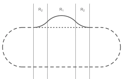
Hausdorff distance and thus need to work over small sets on which the manifold cannot vary too greatly. Hence, we cover the pilot estimator with long, thin slabs R1, . . . ,RN. We do this by

first coveringM with spherese ג_{1, . . . ,}ג_{N of radius}δ_{n=O((log n/n)}1/(2+d)_{). We define a slab}

Rjto be the union of fibers of size b=σ+anwithin one of the spheres: Rj=∪x∈גjLb(x,Me). We then show that:

b. As M cuts through a slab, it stays nearly parallel toM. Roughly speaking, M behavese

like a smooth, nearly linear function within each slab. (Lemma 16).

Step 4. Using the second half of the data, we apply maximum likelihood within each slab. This

defines estimatorsMbj, for 1≤j≤N. We show that:

a. The entropy of the set of distributions within a slab is very small. (Lemma 18). b. Because the entropy is small, the maximum likelihood estimator within a slab

con-verges fairly quickly in Hellinger distance. The rate isεn= (log n/n)1/(2+d). (Lemma

19).

c. Within a slab, there is a tight relationship between Hellinger distance and Hausdorff

distance. Specifically, H(M1,M2)≤c h2(Q1,Q2). (Lemma 20).

d. Steps (4b) and (4c) imply that H(M_∩Rj,Mbj) =OP(ε2n) =OP((log n/n)2/(d+2)).

Step 5. Finally we defineMb=SN_j=1Mbjand show thatM converges at the optimal rate because eachb

b

Mj does within its own slab.

The reason for getting a preliminary estimator and then covering the estimator with thin slabs is that, within a slab, there is a tight relationship between Hellinger distance and Hausdorff distance. This is not true globally but only in thin slabs. Maximum likelihood is optimal with respect to Hellinger distance. Within a slab, this allows us to get optimal rates in Hausdorff distance.

4.3 Step 1: Data Splitting

For simplicity assume the sample size is even and denote it by 2n. We split the data into two halves which we denote by X = (X1, . . . ,Xn)and Y = (Y1, . . . ,Yn).

4.4 Step 2: Pilot Estimator

Let eq be the maximum likelihood estimator over

Q

. Let M be the corresponding manifold. Toe

study the properties ofM requires two steps: computing the bracketing entropy ofe

Q

and relating

H(M,Me)to h(q,_eq). The former allows us to apply Theorem 7 to bound h(q,q_e), and the latter allows us to control the Hausdorff distance.

4.5 Step 2a: Computing the Entropy of

Q

To compute the entropy of

Q

we start by constructing a finite net of manifolds to cover

M

(κ). A finite set of d-manifoldsM_{γ={M1, . . . ,MN}is a}γ_{-net (or a}γ_{-cover) if, for each M∈}

_M

_{there exists}

Mj ∈Mγsuch that H(M,Mj)≤γ. Let N(γ) =N(γ,

M

,H)be the size of the smallest covering set,

called the (Hausdorff) covering number of

M

.

Theorem 9 The Hausdorff covering number of

M

satisfies the following:

N(γ)_≡N(γ,

M

,H)_≤c1κ2(κ,d,D)exp

κ3(κ,d,D)γ−d/2_≡c exp

c′γ−d/2

whereκ2(κ,d,D) = D_d(c2/κ) D

Proof Recall that the manifolds in

M

all lie within

K

. Consider any hypercube containing

K

. Divide this cube into a grid of J= (2c/κ)D_sub-cubes{C

1, . . . ,CJ}of side lengthκ/c, where c≥4

is a positive constant chosen to be sufficiently large. Our strategy is to show that within each of these cubes, the manifold is the graph of a smooth function. We then only need count the number of such smooth functions.

In thinking about the manifold as (locally) the graph of a smooth function, it helps to be able to translate easily between the natural coordinates in

K

and the domain-range coordinates of the function. To that end, within each subcube Cj for j∈ {1, . . . ,J}, we define K= D_d

coordinate frames, Fjk for k∈ {1, . . . ,K}, in which d out of D coordinates are labeled as “domain” and the

remaining D₋d coordinates are labeled as “range.”

Each frame is associated with a relabeling of the coordinates so that the d “domain” coordinates are listed first and D₋d “range” coordinates last. That is, Fjk is defined by a one-to-one

corre-spondence between x_∈Cj and(u,v)∈πjk(x) where u∈Rd and v∈RD−d andπjk(x1, . . . ,xD) =

(xi1, . . . ,xid,xj1, . . . ,xjD−d)for domain coordinate indices i1< . . . <id and range coordinate indices

j1< . . . < jD−d.

We define domain(Fjk) ={u∈Rd : ∃v∈RD−d such that(u,v)∈Fjk}, and let

G

jk denote the

class of functions defined on domain(Fjk)whose second derivative (i.e., second fundamental form)

is bounded above by a constant C(κ)that depends only onκ. To say that a set R_⊂Cjis the graph of

a function on a d-dimensional subset of the coordinates in Cj is equivalent to saying that for some

frame Fjkand some set A⊂domain(Fjk), R=π−_jk1{(u,f(u)): u∈A}.

We will prove the theorem by establishing the following claims.

Claim 1. Let M _∈

M

and Cj be a subcube that intersects M. Then: (i) for at least one k ∈ {1, . . . ,K_}, the set M_∩Cj is the graph of a function (i.e., single-valued mapping) defined on a

set

A

⊂domain(Fjk), of the form (u1, . . . ,ud)7→π−jk1((u,f(u))) for some function f on

A

, and

(ii) this function lies in

G

jk.

Claim 2.

M

is in one-to-one correspondence with a subset of

G

=∏J_j=1SK_k=1

G

jk.

Claim 3. The L∞covering number of

G

satisfies

N(γ,

G

,L∞)_≤c1

D d

(2c/κ)D

exp(D₋d)(2c/κ)D_γ−d/2_.

Claim 4. There is a one-to-one correspondence between anγ/2 L∞-cover of

G

and anγ Hausdorff-cover of

M

.

Taken together, the claims imply that

N(γ,

M

,H)_≤c1

D d

(2c/κ)D

exp((D−d)(2c/κ)D₂d/2_γ−d/2_).

Taking c2=2c proves the theorem.

Proof of Claim 1. We begin by showing that (i) implies (ii). By part 1 of Lemma 3, each M_∈

M

has curvature (second fundamental form) bounded above by 1/κ. This implies that the function identified in (i) has uniformly bounded second derivative and thus lies in the corresponding

G

jk.

We prove (i) by contradiction. Suppose that there is an M _∈

M

such that for every j with

M_∩Cj 6=/0, the set M∩Cj is not the graph of a single-valued mapping for any of the K coordinate

Fix j∈ {1, . . . ,J}. Then in each domain(Fjk), there is a point u such that Cj∩π−_jk1(u×RD−d)

intersects M in at least two points, call them ak and bk. By constructionkak−bkk ≤ √

D₋d_·κ/c,

and hence by choosing c large enough (making the cubes small), part 3 of Lemma 3 tells us that

dM(ak,bk)≤2 √

D₋dκ/c. Then we argue as follows:

1. By parts 2 and 3 of Lemma 3 and the fact that Cjhas diameter √

Dκ/c and

max

p,q∈Cj∩M

cos(angle(TpM,TqM))≥1−

2√D c .

For large enough c, the maximum angle between tangent vectors can be made smaller than

π/3.

2. By part 2 of Lemma 3, any point z along a geodesic between akand bk,

cos(angle(TakM,TzM))≥1−

2√D₋d c .

It follows that there is a point in Cj∩M and a tangent vector vk at that point such that

angle(vk,bk−ak) =O(1/√c).

3. We have for each of K= D_dcoordinate frames and associated tangent vectors v1, . . . ,vKthat

are each nearly orthogonal to at least d of the others. Consequently, there are_≥d+1 nearly orthogonal tangent vectors of M within Cj. This contradicts point 1 and proves the claim.

Proof of Claim 2. We construct the correspondence as follows. For each cube Cj, let k∗j be

the smallest k such that M_∩Cj is the graph of a function φjk∈

G

jk as in Claim 1. Map M to ϕ= (φ1k∗

1, . . . ,φJk∗J), and let

F

⊂

G

be the image of this map. If M6=M

′_∈

_M

_{, then the corresponding} ϕ andϕ′ must be distinct. If not, then M_∩Cj =M′∩Cj for all j, contradicting M6=M′. The

correspondence from

M

to

F

is thus a one-to-one correspondence.

Proof of Claim 3. From the results in Birman and Solomjak (1967), the set of functions defined

on a pre-compact d-dimensional set that take values in a fixed dimension spaceRm_{with uniformly}

bounded second derivative has L∞ covering number bounded above by c1em(1/γ)

d/2

for some c1.

Part 1 of Lemma 3 shows that each M_∈

M

has curvature (second fundamental form) bounded above by 1/κ, so each

G

jk satisfies Birman and Solomjak’s conditions. Hence, N(γ,

G

jk,L∞)≤

c1e(D−d)(1/γ)

d/2

. Because all the

G

jk’s are disjoint, simple counting arguments show that N(γ,

G

,L∞) =

D d

N(γ,

G

jk,L∞)

J

, where J is the number of cubes defined above. The claim follows. (Note that the functions in Claim 1 are defined on a subset of domain(Fjk). But because all such functions have

an extension in

G

jk, a covering of

G

jkalso covers these functions defined on restricted domains.)

Proof of Claim 4. First, note that if two functions are less thanγdistant in L∞, their graphs are less thanγdistant in Hausdorff distance, and vice versa. This implies that aγL∞-cover of a set of functions corresponds directly to anγHausdorff-cover of the set of the functions’ graphs. Hence, in the argument that follows, we can work with functions or graphs interchangeably.

For k∈ {1, . . . ,K}, let

G

_jkγ be a minimal L∞cover of

G

jk byγ/2 balls; specifically, we assume

that

G

γ_jk is the set of centers of these balls. For each gjk∈

G

γ_jk, define fjk(u) =π−_jk1(u,gjk(u)).

smooth (smooth within each cube) but may fail to satisfy∆(M′)_≥κglobally. Let

A

be the collection of M′constructed this way. There are N(γ/2,

G

,L∞)elements in this collection.

By construction and Claim 2, for each M∈

M

, there exists an M′∈

A

such that H(M,M′)_≤γ/2. In other words, the set ofγ/2 Hausdorff balls around the manifolds in

A

covers

M

but the elements of

A

are not themselves necessarily in

M

. Let BH(A,γ/2)denote the set of all d-manifolds M∈

M

such that H(A,M)_≤γ/2. Let

A

0=

n

A∈

A

: BH(A,γ/2)∩

M

6=/0

o

.

For each A_∈

A

0, choose someAe∈BH(A,γ/2)∩

M

. By the triangle inequality, the set{A : Ae ∈

A

0}

forms anγHausdorff-net for

M

. This proves the claim.

We are almost ready to compute the entropy. We will need the following lemma.

Lemma 10 Let 0<γ<κ₋σ. There exists a constant K>0 (depending only on

K

,κandσ) such that, for any M1,M2∈

M

(κ), H(M1,M2)≤γimplies that|V(M1⊕σ)−V(M2⊕σ)| ≤Kγ. Also, for any M_∈

M

(κ),_|V(M_⊕(σ+γ))₋V(M_⊕σ)_{| ≤}Kγ.

Proof Let Sj=Mj⊕σ, j=1,2. Then, using (3),

S2⊂M1⊕(σ+γ) =

[

u∈M1

L_σ+γ(u).

Hence, uniformly over

M

,

V(S2)≤

Z

M1

νD₋d(Lσ+γ(u))dµM1 ≤

Z

M1

νD₋d(Lσ(u))dµM1+Kγ=V(S1) +Kγ

sinceνD₋d(B(u,σ+γ))≤νD₋d(B(u,σ)) +Kγfor some K>0 not depending on M1or M2. By a

symmetric argument, V(S1)≤V(S2) +Kγ. Hence,|V(M1⊕σ)−V(M2⊕σ)| ≤Kγ. The second

statement is proved in a similar way.

Now we construct a Hellinger bracketing. Letγ=ε2_{. LetM}

γ={M1, . . . ,MN}be aγ-Hausdorff

net of manifolds. Thus, by Theorem 9, N=N(ε2_,

_M

_,H)≤c

1ec2(1/ε)

d

. Letωdenote the volume of a sphere of radiusσ. Let qjbe the density corresponding to Mj. Define

uj(y) =

qj(y) +

2ε2

V(Mj⊕(σ+ε2))

I(y_∈Mj⊕(σ+ε2))

and

ℓj(y) =

qj(y)−

2ε2

V(Mj⊕(σ−ε2))

I(y_∈Mj⊕(σ−ε2)).

Let

B

=_{(ℓ1,u1), . . . ,(ℓN,uN)}.

Proof Let M∈

M

(κ)and let Q=QMbe the corresponding distribution. Let q be the density of Q. Q

is supported on S=M_⊕σ. There exists Mj∈Mγsuch that H(M,Mj)≤ε2. Let y be in S. Then there

is a x_∈M such that_||y₋x_{|| ≤}σ. There is a x′_∈Mjsuch that||x−x′|| ≤ε2. Hence, d(y,Mj)≤σ+ε2

and thus y is in the support of uj. Now, for y∈S, uj(y)−q(y) =2ε2/V(Mj⊕(σ+ε2))≥0. Hence,

q(y)_≤uj(y). By a similar argument,ℓj(y)≤q(y). Thus

B

is a bracketing. Now

ℓ1(ℓj,uj) =

Z

uj−

Z

ℓj=

1+2Kε

2 ω

−

1₋2Kε

2 ω

=4Kε

2 ω .

Finally, by (1), h(uj, ℓj)≤

p

ℓ1(ℓj,uj) =Cε. Thus

B

is a Cε-Hellinger bracketing.

4.6 Step 2b. Hellinger Rate Lemma 12 LetQ be the mle. Thene

sup

Q∈Q

Qnnh(Q,Qe)>C0n−

1

d+2 o

≤expn₋Cn2+dd

o

.

Proof We have shown (Lemma 11) that

H

[ ](ε,

Q

,h)≤C(1/ε)d. Solving the equation H[ ](εn,

Q

,h) =

nε2_nfrom Theorem 7 we getεn= (1/n)1/(d+2). From Lemma 8, for all Q

Qn

n

h(Q,Qe)>C0n−

1

d+2 o

≤c1e−c2nε

2

n _=exp

n

−Cn2+dd

o

.

4.7 Step 2c. Relating Hellinger Distance and Hausdorff Distance

Lemma 13 Let c= (κ₋σ)√πC_∗/(2Γ(D/2+1)). If M1,M2∈

M

(κ)and h(Q1,Q2)<c then

H(M2,M2)≤

"

2

√_π

_Γ

(D/2+1)

C_∗

1/D#

hD1(_Q1,_Q2)

Proof Let b=H(M1,M2)andγ=min{κ−σ,b}. Let S1,S2be the supports of Q1and Q2. Because H(M1,M2) =b, we can find points x∈M1 and y∈M2such thatky−xk=b. Note that TxM1and TyM2. are parallel, otherwise we could move x or y and increaseky−xk. It follows that the line

segment[x,y]is along a common normal vector of the two manifolds and we can write y=x_±bu

for some u_∈L_σ(u,M). Without loss of generality, assume that y=x+bu. Let x′=x+σu and y′ =y+σu. Hence, x′_∈∂S1, y′∈∂S2 and||x′−y′||=b. Note that ∂S1 and ∂S2 are themselves

smooth D-manifolds with∆(∂Si)≥κ−σ>0.

We now make the following three claims:

1. y′_∈S2−S1.

2. (x′,y′]_⊂S2−S1

3. interior B

x′+y′ 2 ,

γ

2

First, note that y′differs from y along a fiber of M2by exactlyσ, therefore[x′,y′]⊂S2. Second,

because x′_∈∂S1, there is a neighborhood of x′in[x′,y′]that is not contained in S1. Hence, if there is

a point in S1∩[x′,y′]there must be a point z′∈∂S1∩[x′,y′], with z′6=x′. This implies the existence

of two distinct points whose fibers of length less thanκ−σcross, which contradicts the fact that

∆(∂S1)≥κ−σ. Claims 1 and 2 follows.

Let B=Bx′+y₂ ′,γ₂. By construction, B is tangent to ∂S1 at x′ and tangent to ∂S2 at y′, and B contains [x′,y′]. The ball has radiusγ/2= (1/2)min_{κ₋σ,b_}<κ₋σ. Because B intersects

S2−S1, the interior of B cannot intersect either∂S1 or∂S2. Claim 3 follows by a similar argument

as in the proof of Claim 2. (In particular, if there were a point in the interior of B that is either in S1

or outside S2, a line segment from(x′+y′)/2 to that point would have to intersect the corresponding

boundary, which cannot happen.)

Now V(B) = (γ/2)D_πD/2_{/Γ(D/2+1). So}

h(Q1,Q2) ≥ ℓ1(Q1,Q2) =

Z

|q1−q2| ≥

Z

S1∩Sc2

|q1−q2|

= Z

S1∩S2c

q1=Q1(S1∩S2c)≥C∗V(S1∩Sc2) =C∗(γ/2)DπD/2/Γ(D/2+1).

Hence,

γ=min_{κ₋σ,b_{} ≤}

"

2

√_π

_Γ

(D/2+1)

C_∗

1/D#

h1/D(Q1,Q2).

Ifκ₋σ_≤b this implies that h(Q1,Q2)>c which contradicts the assumption that h(Q1,Q2)<c.

Therefore,γ=b and the conclusion follows.

4.8 Step 2d. Computing The Hausdorff Rate of the Pilot Lemma 14 Let an=

C0

n

2

D(d+2)

. For all large n,

sup

Q∈Q

Qn_{H(M,Me)>an}

≤expn₋Cn2+dd

o

.

Proof Follows by combining Lemma 12 and Lemma 13.

We conclude that, with high probability, the true manifold M is contained in the set

Mn

=nM_∈

M

(κ): H(Me,M)_≤an

o

.

4.9 Step 3: Cover With Slabs

Now we cover the pilot estimatorM with (possibly overlapping) slabs. Lete δn=

C log n n

1

2+d . It

follows from part 6 of Lemma 3 that there exists a collection of points F=_{x1, . . . ,xN} ⊂M, suche

Figure 4: Figure for the proof of part 1 of Lemma 15.

4.10 Step 3a. The Fibers ofM Cover M Nicelye

Lemma 15 Let b=σ+an. For xe∈M, let Le b(ex) =T_ex⊥Me∩BD(ex,b)be a fiber atex of size b. Let

M∈

Mn

. Then:

1. Ifex_∈M and xe _∈M are such thatkx₋exk ≤an, thenangle(TxM,TexMe)<π/4.

2. Lb(ex)∩M6=/0.

3. If x_∈Lb(ex)∩M, thenkx−xek ≤2an.

4. For anyex_∈M, #e _{Lb(ex)∩M}=1.

5. We have M_⊂S_ex∈MeLb(ex).

Proof 1. Let x and ex be as given in the statement of the lemma and letθ=angle(TxM,T_exMe).

Suppose that θ_≥π/4. There exists unit vectors u_∈T_exM and ve ∈TxM such that angle(u,v) = θ. Without loss of generality, we can assume that x=_ex. (The extension to the case x6=x is_e

straightforward.)

Consider the plane defined by u and v as in Figure 4. We assume, without loss of generality, that (u+v)/2 generates the x-axis in this plane and that v lies above the x-axis and u lies below the x axis. Letℓdenote the horizontal line, parallel to the x-axis and lying 2anunits above the horizontal

axis. Hence, u and v each make an angle greater thanπ/8 with respect to the x-axis.

Consider the two circles

C

1and

C

2tangent to M at x with radiusκwhere

C

1lies below v and

C

2

lies above v. Let w be the point at which

C

1intersectsℓ. The arclength of

C

1from x to w is Canfor

some C>1. Letγbe the geodesic on M through x with gradient v. The projectionbγofγinto the plane must fall between

C

1and

C

2. Let y=γ(Can)andby be the projection of y into the plane.

Now _||y₋xe_{|| ≥ ||}yb₋ex_{|| ≥ ||}w₋ex_{|| ≥}2an>an. There existsez∈M such thate ||ez−y|| ≤an.

with coordinates(an √

C2_−1,a

n). Thus,||q−ex||=C an. Note thatangle(bz−xe,u)is larger than the

angle between q₋ex and the x-axis which is arctan

1 √

C2₋₁

≡α>0. Hence,

angle(_ez₋x_e,u)_≥angle(_bz₋x_e,u)_≥α.

Leteγbe a geodesic on M, parameterized by arclength connectinge _ex and_ez. Thuseγ(0) =_ex and

eγ(T) =_ez for some T . There exists some 0≤t≤T such thatγ′(t)∝_ez−ex. So

angle(γ′(t),γ′(0)) =α>0.

However,_||ez₋xe_{|| ≤}(C+1)anwhich implies, by part 2 of Lemma 3, thatangle(γ′(t),γ′(0)) =

O(√an)<αwhich is a contradiction.

2. For any_ex_∈M, the closest point xe _∈M must satisfy_kx_−ex_{k ≤}an. Let y be the projection of x

onto T_exM. Let Ue =TxeMe∩Bd(y,an). Let Cyl=Su∈UBD(u,3an)∩

T_exMe

⊥

. Cyl is a small hyper-cylinder containing y and_ex, with the former in the center. M cannot intersect the top or bottom faces

of the cylinder. Otherwise, we can find a point p∈M such thatangle(T_exMe,TpM)>arctan(1) =π/4

contradicting 1. Thus, any path through x on M must intersect the sides of Cyl. Hence, Lb(ex)∩M6= /0.

3. Let x∈M∩Lb(ex). Suppose that||x−ex||>2an. There exists q∈M such thate ||q−x|| ≤an.

Note that_||q₋ex_||>an. Now we apply part 5 Lemma 3 with p=x and ve =x. This implies that ||v₋p_||=_||x_−ex_||<a2_n/κwhich contradicts the assumption that_||x₋x_e||>2an.

4. Suppose that more than one point of M were in Lb(ex). Pick two and call them x1and x2. By 3, kxi−exk ≤2an. It follows thatkx1−x2k ≤4anand thus they are O(an)close in geodesic distance by

part 3 of Lemma 3. Hence, there is a geodesic on M connecting x1and x2that is contained strictly

within the Canball. Because x2−x1lies in Lb(xe)and is consequently orthogonal to TexM, there muste

exist a point on the geodesic whose angle with T_exM equalse π/2, contradicting part 1.

5. Because H(Me,M)_≤an, we have that M⊂tube(Me,an). Because an<κ, the fibers Lb(xe)partition

tube(Me,an). Hence, each x∈M must lie on one (and only one) Lb(ex).

4.11 Step 3b. Construct Slabs that Cover M Nicely

Letג_j=BD(xj,δ_{n)∩M. Define the slab}e

Rj=

[

x∈ג_j

Lb(x,Me).

Lemma 16 The collection of slabs R1, . . . ,RNhas the following properties. Let M∈

Mn

.

1. M_⊂SN_j=1Rj.

2. M_∩Rj is function-like over Rj. That is, there exists a function gj :גj →RD−d such that

M_∩Rj={gj(x): x∈גj}.

3. For each x∈ג_{j, Lb(x)∩M6=}/0_.

5. sup_M∈Mndiam(M∩Rj)≤Cδn.

Thus the slabs cover M and M cuts across Rj is a function-like way. Moreover, M∩Rjis nearly

linear.

Proof The first three claims follow immediately from Lemma 15. In particular, gj in claim 2 is

defined by gj(x) ={M∩Lb(x)}. Now we show 4. We can write gj(x) =gj(xj) + (x−xj)T∇g+ 1

2(x−xj)

T_Hess(x−x

j) whereHess is the Hessian matrix of gj evaluated at some point between

x and xj. By part 1 of Lemma 3, the largest eigenvalue ofHessis bounded above by 1/κ. Since ||x₋xj|| ≤cδ2n, the claim follows. Part 5 follows easily.

4.12 Step 4: Local Conditional Likelihood

Recall that

Mn

=_{M_∈

M

(κ): H(Me,M)_≤an}. Let

Qn

=_{QM: M∈

Mn

}.

Consider a slab Rj. For each Q∈

Qn

define Qj ≡Q(·|Rj)by Qj(A) =Q(A∩Rj)/Q(Rj). Note that

Qj is supported overtube(M,σ)∩Rj. Let

Qn

,j={Qj: Q∈

Qn

}. Before we proceed we need to

establish the following.

Lemma 17 Let

I

j(M) =tube(M,σ)∩Rj. Then there exists c0>0 such that

inf

M_∈Mn

V(

I

j(M))≥c0δdn.

Proof By Lemma 16, M_∩Rj lies in a slab of size an orthogonal toגj. Because the angle between

the two manifolds on this set must be no more than π/4 and because an>δn, the manifold M

cannot intersect both the “top” and “bottom” surfaces of the slab. Hence, for large enough C>0,

J

j=Sx∈גjBD(x,σ/C)⊂

I

j. By construction, V(

Ij

)≥V(

J

j)≥cδ d n.

4.13 Step 4a. The Entropy of

Qn

,j Lemma 18

H

[ ](ε,

Qn

,j,h)≤c1log(c2/ε).

Proof We begin by creating aγHausdorff net for

Qn

,j. To do this, we will parameterize the support

of these distributions. Each Q_∈

Qn

,jhas support in the collection

Sn

,j={(M⊕σ)∩Rj: M∈

Mn

}.

We will construct aγ-Hausdorff net for

Sn

,j.

Let_ex_∈M be the center ofe ג_{j. Let y1, . . . ,yrbe a c}1γ_{-net of Lb(ex), and let}θ1_<θ2_<···<θ_s<

π/2₋ηfor a small, fixedη>0 whereθj−θj−1≤c2γ. Note that r=O(γ−(D−d))and s=O(1/γ).

For every pair yi andθj, let Mi j be a M∈

Mn

that crosses through yi withangle(TyiM,TexMe) =θj. These manifolds comprise a collection of size O((1/γ)D−d−1_{)which we will denote byNet(}γ_).

Let M _∈

Mn

. Let y be the point where M crosses Lb(xe). Let yi be the closest point in the net

to y and letθj be the closest angle in the net toangle(TyM,TexMe). Because the angle between M

and Mi j is strictly less thanπ/4 (part 1 of Lemma 15) and the slab Rj has radiusδn, it follows that

Now considerNet(γ)withγ=ε2_{. For each M}

i j ∈Net(γ) let qi j be the corresponding density

and define ui j andℓi j by

ui j(y) =

qi j(y) +

Cε2 V(Mi j⊕(σ+ε2))

I(y_∈Mi j⊕(σ+ε2))

and

ℓi j(y) =

qi j(y)−

Cε2 V(Mi j⊕(σ−ε2))

I(y_∈Mj⊕(σ−ε2)).

Let

B

=_{(ℓi j,ui j)}.

Let M_∈

Mn

and let Mi j be the element of the net closest to M. It follows easily that ui j≥qM≥

ℓi j. Thus

B

is a bracketing. Now,

Z

ui j−ℓi j=1+Cε2−(1−Cε2) =2Cε2.

Hence, h(ui j, ℓi j)≤

pR

|ui j−ℓi j|= √

2Cε. Hence,

B

is an√2C₋ε-bracketing. So,

H[ ]

(ε,

Qn

,j,h)≤(D−d−1)log(c/ε),

which proves the lemma.

4.14 Step 4b. Hellinger Rate of the Conditional MLE

Letq be the mle over_b

Qn

,j using the Yi’s in Rj. LetM be the manifold corresponding tob q and letb

b

Mj=Mb∩Rj.

Lemma 19 For all Q, all A>0 and all large n,

Qn

(

h(Q,Qb)>

C0log n n

1

2+d

)!

≤n−A.

Proof Let Nj be the number of observations from the second half of the data that are in Rj. Let

µj =E(Nj) and define mn=n

2

2+d_{. First, we claim that Nj} ≥_µj/₂=_O(_mn) _{for all j, except on a} set of probability e−cn2/(2+d). Let πj =Q(Rj). By Lemma 17 and Lemma 4, πj ≥cδdn for some

c>0. Hence, µj≥mn. Note thatσ2≡Var(Nj)/n=πj(1−πj)≤πj. Let t=µj/2. By Bernstein’s

inequality,

P_{(Nj≤µj/2) =}P_{(Nj−µj≤ −µj/2)≤exp}

− t

2

2nσ2_+2t/3

≤exp

n

−cn2/(2+d)

o

.

Hence, by the union bound,

P_{(Nj≤µj/2 for some j)≤} 1

Nexp

n

−cn2/(2+d)

o

≤exp

n

−c′n2/(2+d)

o

since there are N=O(1/δn)slabs. Thus we can assume that there are at least order mnobservations