A Tutorial on Conformal Prediction

A Tutorial on Conformal Prediction

Glenn Shafer∗ [email protected]

Department of Accounting and Information Systems Rutgers Business School

180 University Avenue Newark, NJ 07102, USA

Vladimir Vovk [email protected]

Computer Learning Research Centre Department of Computer Science Royal Holloway, University of London Egham, Surrey TW20 0EX, UK

Editor: Sanjoy Dasgupta

Abstract

Conformal prediction uses past experience to determine precise levels of confidence in new pre-dictions. Given an error probabilityε, together with a method that makes a prediction ˆy of a label y, it produces a set of labels, typically containing ˆy, that also contains y with probability 1−ε. Conformal prediction can be applied to any method for producing ˆy: a nearest-neighbor method, a

support-vector machine, ridge regression, etc.

Conformal prediction is designed for an on-line setting in which labels are predicted succes-sively, each one being revealed before the next is predicted. The most novel and valuable feature of conformal prediction is that if the successive examples are sampled independently from the same distribution, then the successive predictions will be right 1−εof the time, even though they are based on an accumulating data set rather than on independent data sets.

In addition to the model under which successive examples are sampled independently, other on-line compression models can also use conformal prediction. The widely used Gaussian linear model is one of these.

This tutorial presents a self-contained account of the theory of conformal prediction and works through several numerical examples. A more comprehensive treatment of the topic is provided in

Algorithmic Learning in a Random World, by Vladimir Vovk, Alex Gammerman, and Glenn Shafer

(Springer, 2005).

Keywords: confidence, on-line compression modeling, on-line learning, prediction regions

1. Introduction

How good is your prediction ˆy? If you are predicting the label y of a new object, how confident are you that y=y? If the label y is a number, how close do you think it is to ˆˆ y? In machine learning, these questions are usually answered in a fairly rough way from past experience. We expect new predictions to fare about as well as past predictions.

Conformal prediction uses past experience to determine precise levels of confidence in predic-tions. Given a method for making a prediction ˆy, conformal prediction produces a 95% prediction

region—a setΓ0.05 that contains y with probability at least 95%. TypicallyΓ0.05also contains the prediction ˆy. We call ˆy the point prediction, and we callΓ0.05the region prediction. In the case of regression, where y is a number,Γ0.05is typically an interval around ˆy. In the case of classification, where y has a limited number of possible values,Γ0.05 may consist of a few of these values or, in the ideal case, just one.

Conformal prediction can be used with any method of point prediction for classification or re-gression, including support-vector machines, decision trees, boosting, neural networks, and Bayesian prediction. Starting from the method for point prediction, we construct a nonconformity measure, which measures how unusual an example looks relative to previous examples, and the conformal algorithm turns this nonconformity measure into prediction regions.

Given a nonconformity measure, the conformal algorithm produces a prediction regionΓε for every probability of errorε. The regionΓεis a(1−ε)-prediction region; it contains y with probabil-ity at least 1−ε. The regions for differentεare nested: whenε1≥ε2, so that 1−ε1is a lower level of confidence than 1−ε2, we haveΓε1 _⊆Γε2_{. If}Γε_{contains only a single label (the ideal outcome} in the case of classification), we may ask how smallεcan be made before we must enlargeΓε by adding a second label; the corresponding value of 1−εis the confidence we assert in the predicted label.

As we explain in §4, the conformal algorithm is designed for an on-line setting, in which we predict the labels of objects successively, seeing each label after we have predicted it and before we predict the next one. Our prediction ˆyn of the nth label yn may use observed features xn of the

nth object and the preceding examples(x1,y1), . . . ,(xn−1,yn−1). The size of the prediction regionΓε may also depend on these details. Readers most interested in implementing the conformal algorithm may wish to look first at the elementary examples in §4.2.1 and §4.3.1 and then turn back to the earlier more general material as needed.

As we explain in §2, the on-line picture leads to a new concept of validity for prediction with confidence. Classically, a method for finding 95% prediction regions was considered valid if it had a 95% probability of containing the label predicted, because by the law of large numbers it would then be correct 95% of the time when repeatedly applied to independent data sets. But in the on-line picture, we repeatedly apply a method not to independent data sets but to an accumulating data set. After using(x1,y1), . . . ,(xn−1,yn−1) and xn to predict yn, we use(x1,y1), . . . ,(xn−1,yn−1),(xn,yn)

and xn+1to predict yn+1, and so on. For a 95% on-line method to be valid, 95% of these predictions must be correct. Under minimal assumptions, conformal prediction is valid in this new and powerful sense.

One setting where conformal prediction is valid in the new on-line sense is the one in which the examples (xi,yi)are sampled independently from a constant population—that is, from a fixed but

unknown probability distribution Q. It is also valid under the slightly weaker assumption that the examples are probabilistically exchangeable (see §3) and under other on-line compression models, including the widely used Gaussian linear model (see §5). The validity of conformal prediction under these models is demonstrated in Appendix A.

In addition to the validity of a method for producing 95% prediction regions, we are also inter-ested in its efficiency. It is efficient if the prediction region is usually relatively small and therefore informative. In classification, we would like to see a 95% prediction region so small that it contains only the single predicted label ˆyn. In regression, we would like to see a very narrow interval around

The claim of 95% confidence for a 95% conformal prediction region is valid under exchange-ability, no matter what the probability distribution the examples follow and no matter what non-conformity measure is used to construct the conformal prediction region. But the efficiency of conformal prediction will depend on the probability distribution and the nonconformity measure. If we think we know the probability distribution, we may choose a nonconformity measure that will be efficient if we are right. If we have prior probabilities for Q, we may use these prior probabilities to construct a point predictor ˆyn and a nonconformity measure. In the regression case, we might

use as ˆyn the mean of the posterior distribution for yn given the first n−1 examples and xn; in the

classification case, we might use the label with the greatest posterior probability. This strategy of first guaranteeing validity under a relatively weak assumption and then seeking efficiency under stronger assumptions conforms to advice long given by John Tukey and others (Tukey, 1986; Small et al., 2006).

Conformal prediction is studied in detail in Algorithmic Learning in a Random World, by Vovk, Gammerman, and Shafer (2005). A recent exposition by Gammerman and Vovk (2007) emphasizes connections with the theory of randomness, Bayesian methods, and induction. In this article we emphasize the on-line concept of validity, the meaning of exchangeability, and the generalization to other on-line compression models. We leave aside many important topics that are treated in Algorithmic Learning in a Random World, including extensions beyond the on-line picture.

2. Valid Prediction Regions

Our concept of validity is consistent with a tradition that can be traced back to Jerzy Neyman’s introduction of confidence intervals for parameters (Neyman, 1937) and even to work by Laplace and others in the late 18th century. But the shift of emphasis to prediction (from estimation of parameters) and to the on-line setting (where our prediction rule is repeatedly updated) involves some rearrangement of the furniture.

The most important novelty in conformal prediction is that its successive errors are probabilis-tically independent. This allows us to interpret “being right 95% of the time” in an unusually direct way. In §2.1, we illustrate this point with a well-worn example, normally distributed random vari-ables.

In §2.2, we contrast confidence with full-fledged conditional probability. This contrast has been the topic of endless debate between those who find confidence methods informative (classical statisticians) and those who insist that full-fledged probabilities based on all one’s information are always preferable, even if the only available probabilities are very subjective (Bayesians). Because the debate usually focuses on estimating parameters rather than predicting future observations, and because some readers may be unaware of the debate, we take the time to explain that we find the concept of confidence useful for prediction in spite of its limitations.

2.1 An Example of Valid On-Line Prediction

A 95% prediction region is valid if it contains the truth 95% of the time. To make this more precise, we must specify the set of repetitions envisioned. In the on-line picture, these are successive predictions based on accumulating information. We make one prediction after another, always knowing the outcome of the preceding predictions.

Random variables z1,z2, . . . are independently drawn from a normal distribution with unknown mean and variance.

Prediction under this assumption was discussed in 1935 by R. A. Fisher, who explained how to give a 95% prediction interval for znbased on z1, . . . ,zn−1that is valid in our sense. We will state Fisher’s prediction rule, illustrate its application to data, and explain why it is valid in the on-line setting.

As we will see, the predictions given by Fisher’s rule are too weak to be interesting from a modern machine-learning perspective. This is not surprising, because we are predicting zn based

on old examples z1, . . . ,zn−1alone. In general, more precise prediction is possible only in the more favorable but more complicated set-up where we know some features xnof the new example and can

use both xn and the old examples to predict some other feature yn. But the simplicity of the set-up

where we predict znfrom z1, . . . ,zn−1alone will help us make the logic of valid prediction clear. 2.1.1 FISHER’SPREDICTIONINTERVAL

Suppose we observe the zi in sequence. After observing z1 and z2, we start predicting; for n= 3,4, . . ., we predict znafter having seen z1, . . . ,zn−1. The natural point predictor for znis the average

so far:

zn−1:= 1 n−1

n−1

∑

zi,

but we want to give an interval that will contain zn95% of the time. How can we do this? Here is

Fisher’s answer (1935):

1. In addition to calculating the average zn−1, calculate

s2_n−1:= 1 n−2

n−1

∑

(zi−zn−1)2,

which is sometimes called the sample variance. We can usually assume that it is non-zero.

2. In a table of percentiles for t-distributions, find t_n0₋₂.025, the point that the t-distribution with n−2 degrees of freedom exceeds exactly 2.5% of the time.

3. Predict that znwill be in the interval

zn−1±tn0−2.025sn−1

r

n

n−1. (1)

Fisher based this procedure on the fact that

zn−zn−1 sn−1

r

n−1 n

2.1.2 A NUMERICALEXAMPLE

We can illustrate (1) using some numbers generated in 1900 by the students of Emanuel Czuber (1851–1925). These numbers are integers, but they theoretically have a binomial distribution and are therefore approximately normally distributed.1

Here are Czuber’s first 19 numbers, z1, . . . ,z19:

17,20,10,17,12,15,19,22,17,19,14,22,18,17,13,12,18,15,17.

From them, we calculate

z19=16.53, s19=3.31.

The upper 2.5% point for the t-distribution with 18 degrees of freedom, t₁₈0.025, is 2.101. So the prediction interval (1) for z20comes out to[9.40,24.13].

Taking into account our knowledge that z20will be an integer, we can say that the 95% prediction is that z20will be an integer between 10 and 24, inclusive. This prediction is correct; z20is 16. 2.1.3 ON-LINE VALIDITY

Fisher did not have the on-line picture in mind. He probably had in mind a picture where the for-mula (1) is used repeatedly but in entirely separate problems. For example, we might conduct many separate experiments that each consists of drawing 100 random numbers from a normal distribution and then predicting a 101st draw using (1). Each experiment might involve a different normal dis-tribution (a different mean and variance), but provided the experiments are independent from each other, the law of large numbers will apply. Each time the probability is 95% that z101will be in the interval, and so this event will happen approximately 95% of the time.

The on-line story may seem more complicated, because the experiment involved in predicting z101 from z1, . . . ,z100is not entirely independent of the experiment involved in predicting, say, z105 from z1, . . . ,z104. The 101 random numbers involved in the first experiment are all also involved in the second. But as a master of the analytical geometry of the normal distribution (Fisher, 1925; Efron, 1969), Fisher would have noticed, had he thought about it, that this overlap does not actually matter. As we show in Appendix A.3, the events

zn−1−tn0−2.025sn−1

r

n

n−1 ≤zn≤zn−1+t 0.025

n−2 sn−1

r

n

n−1 (2)

for successive n are probabilistically independent in spite of the overlap. Because of this indepen-dence, the law of large numbers again applies. Knowing each event has probability 95%, we can conclude that approximately 95% of them will happen. We call the events (2) hits.

The prediction interval (1) generalizes to linear regression with normally distributed errors, and on-line hits remain independent in this general setting. Even though formulas for these linear-regression prediction intervals appear in textbooks, the independence of their on-line hits was not noted prior to our work on conformal prediction. Like Fisher, the textbook authors did not have the

1. Czuber’s students randomly drew balls from an urn containing six balls, numbered 1 to 6. Each time they drew a ball, they noted its label and put it back in the urn. After each 100 draws, they recorded the number of times that the ball labeled with a 1 was drawn (Czuber, 1914, pp. 329–335). This should have a binomial distribution with parameters 100 and 1/6, and it is therefore approximately normal with mean 100/6=16.67 and standard deviation

p

on-line setting in mind. They imagined just one prediction being made in each case where data is accumulated.

We will return to the generalization to linear regression in §5.3.2. There we will derive the textbook intervals as conformal prediction regions within the on-line Gaussian linear model, an on-line compression model that uses slightly weaker assumptions than the classical assumption of independent and normally distributed errors.

2.2 Confidence Says Less than Probability.

Neyman’s notion of confidence looks at a procedure before observations are made. Before any of the ziare observed, the event (2) involves multiple uncertainties: zn−1, sn−1, and znare all uncertain.

The probability that these three quantities will turn out so that (2) holds is 95%.

We might ask for more than this. It is after we observe the first n−1 examples that we calculate zn−1and sn−1and then calculate the interval (1), and we would like to be able to say at this point that there is still a 95% probability that znwill be in (1). But this, it seems, is asking for too much. The

assumptions we have made are insufficient to enable us to find a numerical probability for (2) that will be valid at this late date. In theory there is a conditional probability for (2) given z1, . . . ,zn−1, but it involves the unknown mean and variance of the normal distribution.

Perhaps the matter is best understood from the game-theoretic point of view. A probability can be thought of as an offer to bet. A 95% probability, for example, is an offer to take either side of a bet at 19 to 1 odds. The probability is valid if the offer does not put the person making it at a disadvantage, inasmuch as a long sequence of equally reasonable offers will not allow an opponent to multiply the capital he or she risks by a large factor (Shafer and Vovk, 2001). When we assume a probability model (such as the normal model we just used or the on-line compression models we will study later), we are assuming that the model’s probabilities are valid in this sense before any examples are observed. Matters may be different afterwards.

In general, a 95% conformal predictor is a rule for using the preceding examples(x1,y1), . . . ,

(xn−1,yn−1)and a new object xnto give a set, say

Γ0.05_((x

1,y1), . . . ,(xn−1,yn−1),xn), (3)

that we predict will contain yn. If the predictor is valid, the prediction

yn∈Γ0.05((x1,y1), . . . ,(xn−1,yn−1),xn)

will have a 95% probability before any of the examples are observed, and it will be safe, at that point, to offer 19 to 1 odds on it. But after we observe(x1,y1), . . . ,(xn−1,yn−1)and xnand calculate

the set (3), we may want to withdraw the offer.

Particularly striking instances of this phenomenon can arise in the case of classification, where there are only finitely many possible labels. We will see one such instance in §4.3.1, where we consider a classification problem in which there are only two possible labels, s and v. In this case, there are only four possibilities for the prediction region:

1. Γ0.05_((x

1,y1), . . . ,(xn−1,yn−1),xn)contains only s.

2. Γ0.05((x1,y1), . . . ,(xn−1,yn−1),xn)contains only v.

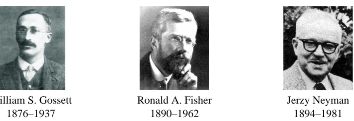
William S. Gossett 1876–1937

Ronald A. Fisher 1890–1962

Jerzy Neyman 1894–1981

Figure 1: Three influential statisticians. Gossett, who worked as a statistician for the Guinness brewery in Dublin, introduced the t-distribution to English-speaking statisticians (Stu-dent, 1908). Fisher, whose applied and theoretical work invigorated mathematical statis-tics in the 1920s and 1930s, refined, promoted, and extended Gossett’s work. Neyman was one of the most influential leaders in the subsequent movement to use advanced prob-ability theory to give statistics a firmer foundation and further extend its applications.

4. Γ0.05((x1,y1), . . . ,(xn−1,yn−1),xn)is empty.

The third and fourth cases can occur even though Γ0.05 is valid. When the third case happens, the prediction, though uninformative, is certain to be correct. When the fourth case happens, the prediction is clearly wrong. These cases are consistent with the prediction being right 95% of the time. But when we see them arise, we know whether the particular value of n is one of the 95% where we are right or the one of the 5% where we are wrong, and so the 95% will not remain valid as a probability defining betting odds.

In the case of normally distributed examples, Fisher called the 95% probability for znbeing in

the interval (1) a “fiducial probability,” and he seems to have believed that it would not be susceptible to a gambling opponent who knows the first n−1 examples (see Fisher, 1973, pp. 119–125). But this turned out not to be the case (Robinson, 1975). For this and related reasons, most scientists who use Fisher’s methods have adopted the interpretation offered by Neyman, who wrote about “confidence” rather than fiducial probability and emphasized that a confidence level is a full-fledged probability only before we acquire data. It is the procedure or method, not the interval or region it produces when applied to particular data, that has a 95% probability of being correct.

Neyman’s concept of confidence has endured in spite of its shortcomings. It is widely taught and used in almost every branch of science. Perhaps it is especially useful in the on-line setting. It is useful to know that 95% of our predictions are correct even if we cannot assert a full-fledged 95% probability for each prediction when we make it.

3. Exchangeability

Consider variables z1, . . . ,zN. Suppose that for any collection of N values, the N! different orderings

are equally likely. Then we say that z1, . . . ,zN are exchangeable. The assumption that z1, . . . ,zN

In our book (Vovk et al., 2005), conformal prediction is first explained under the assumption that z1, . . . ,zN are independently drawn from a probability distribution (or that they are “random,”

as we say there), and then it is pointed out that this assumption can be relaxed to the assumption that z1, . . . ,zN are exchangeable. When we introduce conformal prediction in this article, in §4, we

assume only exchangeability from the outset, hoping that this will make the logic of the method as clear as possible. Once this logic is clear, it is easy to see that it works not only for the exchange-ability model but also for other on-line compression models (§5).

In this section we look at the relationship between exchangeability and independence and then give a backward-looking definition of exchangeability that can be understood game-theoretically. We conclude with a law of large numbers for exchangeable sequences, which will provide the basis for our confidence that our 95% prediction regions are right 95% of the time.

3.1 Exchangeability and Independence

Although the definition of exchangeability we just gave may be clear enough at an intuitive level, it has two technical problems that make it inadequate as a formal mathematical definition: (1) in the case of continuous distributions, any specific values for z1, . . . ,zNwill have probability zero, and (2)

in the case of discrete distributions, two or more of the zimight take the same value, and so a list of

possible values a1, . . . ,aN might contain fewer than n distinct values.

One way of avoiding these technicalities is to use the concept of a permutation, as follows:

Definition of exchangeability using permutations. The variables z1, . . . ,zN are

ex-changeable if for every permutationτof the integers 1, . . . ,N, the variables w1, . . . ,wN,

where wi=zτ(i), have the same joint probability distribution as z1, . . . ,zN.

We can extend this to a definition of exchangeability for an infinite sequence of variables: z1,z2, . . . are exchangeable if z1, . . . ,zN are exchangeable for every N.

This definition makes it easy to see that independent and identically distributed random variables are exchangeable. Suppose z1, . . . ,zN all take values from the same example space Z, all have the

same probability distribution Q, and are independent. Then their joint distribution satisfies

Pr(z1∈A1&. . . & zN∈AN) =Q(A1)· · ·Q(AN)

for any2 subsets A1, . . . ,AN of Z, where Q(A) is the probability Q assigns to an example being

in A. Because permuting the factors Q(An) does not change their product, and because a joint

probability distribution for z1, . . . ,zN is determined by the probabilities it assigns to events of the

form{z1∈A1&. . . & zN∈AN}, this makes it clear that z1, . . . ,zN are exchangeable.

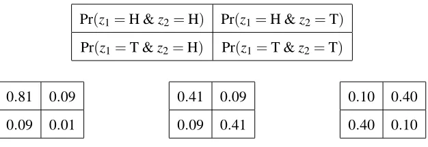
Exchangeability implies that variables have the same distribution. On the other hand, exchange-able variexchange-ables need not be independent. Indeed, when we average two or more distinct joint proba-bility distributions under which variables are independent, we usually get a joint probaproba-bility distribu-tion under which they are exchangeable (averaging preserves exchangeability) but not independent (averaging usually does not preserve independence). According to a famous theorem by de Finetti, an exchangeable joint distribution for an infinite sequence of distinct variables is exchangeable only if it is a mixture of joint distributions under which the variables are independent (Hewitt and Savage, 1955). As Table 1 shows, the picture is more complicated in the finite case.

Pr(z1=H & z2=H) Pr(z1=H & z2=T) Pr(z1=T & z2=H) Pr(z1=T & z2=T)

0.81 0.09

0.09 0.01

0.41 0.09

0.09 0.41

0.10 0.40

0.40 0.10

Table 1: Examples of exchangeability. We consider variables z1and z2, each of which comes out H or T. Exchangeability requires only that Pr(z1=H & z2=T) =Pr(z1=T & z2=H).Three examples of distributions for z1 and z2 with this property are shown. On the left, z1and z2are independent and identically distributed; both come out H with probability 0.9. The middle example is obtained by averaging this distribution with the distribution in which the two variables are again independent and identically distributed but T’s probability is 0.9. The distribution on the right, in contrast, cannot be obtained by averaging distributions under which the variables are independent and identically distributed. Examples of this last type disappear as we ask for a larger and larger number of variables to be exchangeable.

3

4

4

3

4

7

7

7

7

4

Figure 2: Ordering the tiles. Joe gives Bill a bag containing five tiles, and Bill arranges them to form the list 43477. Bill can calculate conditional probabilities for which zi had

which of the five values. His conditional probability for z5=4, for example, is 2/5. There are (5!)/(2!)(2!) =30 ways of assigning the five values to the five variables;

(z1,z2,z3,z4,z5) = (4,3,4,7,7) is one of these, and they all have the same probability, 1/30.

3.2 Backward-Looking Definitions of Exchangeability

Another way of defining exchangeability looks backwards from a situation where we know the unordered values of z1, . . . ,zN.

Suppose Joe has observed z1, . . . ,zN. He writes each value on a tile resembling those used in

Scrabblec, puts the N tiles in a bag, shakes the bag, and gives it to Bill to inspect. Bill sees the N values (some possibly equal to each other) without knowing their original order. Bill also knows the joint probability distribution for z1, . . . ,zN. So he obtains probabilities for the ordering of the tiles by

To make this into a definition of exchangeability, we formalize the notion of a bag. A bag (or multiset, as it is sometimes called) is a collection of elements in which repetition is allowed. It is like a set inasmuch as its elements are unordered but like a list inasmuch as an element can occur more than once. We write *a1, . . . ,aN+ for the bag obtained from the list a1, . . . ,aN by removing

information about the ordering.

Here are three equivalent conditions on the joint distribution of a sequence of random variables z1, . . . ,zN, any of which can be taken as the definition of exchangeability.

1. For any bag B of size N, and for any examples a1, . . . ,aN,

Pr(z1=a1&. . . & zN=aN|*z1, . . . ,zN+=B)

is equal to the probability that successive random drawings from the bag B without replace-ment produces first aN, then aN−1, and so on, until the last element remaining in the bag is a1.

2. For any n, 1≤n≤N, znis independent of zn+1, . . . ,zNgiven the bag*z1, . . . ,zn+and for any

bag B of size n,

Pr(zn=a|*z1, . . . ,zn+=B) =

k

n, (4)

where k is the number of times a occurs in B.

3. For any bag B of size N, and for any examples a1, . . . ,aN,

Pr(z1=a1&. . . & zN =aN|*z1, . . . ,zN+=B) = (_n1!···n

k!

N! if B=*a1, . . . ,aN+

0 if B6=*a1, . . . ,aN+,

(5)

where k is the number of distinct values among the ai, and n1, . . . ,nk are the respective

num-bers of times they occur. (If the ai are all distinct, the expression n1!· · ·nk!/(N!)reduces to

1/(N!).)

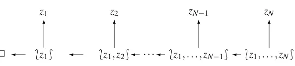
We leave it to the reader to verify that these three conditions are equivalent to each other. The second condition, which we will emphasize, is represented pictorially in Figure 3.

The backward-looking conditions are also equivalent to the definition of exchangeability using permutations given on p. 378. This equivalence is elementary in the case where every possible sequence of values a1, . . . ,anhas positive probability. But complications arise when this probability

is zero, because the conditional probability on the left-hand side of (5) is then defined only with probability one by the joint distribution. We do not explore these complications here.

3.3 The Betting Interpretation of Exchangeability

2 *z1+ *z1,z2+ · · · *z1, . . . ,zN−1+ *z1, . . . ,zN+

z1 z2 zN−1 zN

6 6 6 6

Figure 3: Backward probabilities, step by step. The two arrows backwards from each bag

*z1, . . . ,zn+ symbolize drawing an example zn out at random, leaving the smaller bag

*z1, . . . ,zn−1+. The probabilities for the result of the drawing are given by (4). Readers familiar with Bayes nets (Cowell et al., 1999) will recognize this diagram as an exam-ple; conditional on each variable, a joint probability distribution is given for its children (the variables to which arrows from it point), and given the variable, its descendants are independent of its ancestors.

By applying this idea to the sequence of probabilities (4), we obtain a betting interpretation of exchangeability. Think of Joe and Bill as two players in a game that moves backwards from point N in Figure 3. At each step, Joe provides new information and Bill bets. Designate by

K

capital Bill risks. He begins with this capital at N, and at each step n he bets on what znwill turn

out to be. When he bets at step n, he cannot risk losing more than he has at that point (because he is not risking more than

K

against each possible value a for znat the odds(k/n):(1−k/n), where k is the number of elements

in the current bag equal to a.

For brevity, we write Bnfor the bag*z1, . . . ,zn+, and for simplicity, we set the initial capital KN

equal to $1. This gives the following protocol:

THEBACKWARD-LOOKINGBETTINGPROTOCOL

Players: Joe, Bill

K

Joe announces a bag BNof size N.

FOR n=N,N−1, . . . ,2,1

Bill bets on znat odds set by (4).

Joe announces zn∈Bn.

K

K

Bn−1:=Bn\*zn+.

Constraint: Bill must move so that his capital

K

moves.

Our betting interpretation of exchangeability is that Bill will not multiply his initial capital

K

large factor in this game.

The permutation definition of exchangeability does not lead to an equally simple betting inter-pretation, because the probabilities for z1, . . . ,zN to which the permutation definition refers are not

3.4 A Law of Large Numbers for Exchangeable Sequences

As we noted when we studied Fisher’s prediction interval in §2.1.3, the validity of on-line prediction requires more than having a high probability of a hit for each individual prediction. We also need a law of large numbers, so that we can conclude that a high proportion of the high-probability predictions will be correct. As we show in §A.3, the successive hits in the case of Fisher’s region predictor are independent, so that the usual law of large numbers applies. What can we say in the case of conformal prediction under exchangeability?

Suppose z1, . . . ,zNare exchangeable, drawn from an example space Z. In this context, we adopt

the following definitions.

• An event E is an n-event, where 1≤n≤N, if its happening or failing is determined by the value of znand the value of the bag*z1, . . . ,zn−1+.

• An n-event E isε-rare if

Pr(E|*z1, . . . ,zn+)≤ε. (6)

The left-hand side of the inequality (6) is a random variable, because the bag*z1, . . . ,zn+is random.

The inequality says that this random variable never exceedsε.

As we will see in the next section, the successive errors for a conformal predictor are ε-rare n-events. So the validity of conformal prediction follows from the following informal proposition.

Informal Proposition 1 Suppose N is large, and the variables z1, . . . ,zN are exchangeable.

Sup-pose Enis anε-rare n-event for n=1, . . . ,N. Then the law of large numbers applies; with very high

probability, no more than approximately the fractionεof the events E1, . . . ,EN will happen.

In Appendix A, we formalize this proposition in two ways: classically and game-theoretically. The classical approach appeals to the classical weak law of large numbers, which tells us that if E1, . . . ,EN are mutually independent and each have probability exactlyε, and N is sufficiently large,

then there is a very high probability that the fraction of the events that happen will be close toε. We show in §A.1 that if (6) holds with equality, then Enare mutually independent and each of them has

unconditional probabilityε. Having the inequality instead of equality means that the En are even

less likely to happen, and this will not reverse the conclusion that few of them will happen.

The game-theoretic approach is more straightforward, because the game-theoretic version law of large numbers does not require independence or exact levels of probability. In the game-theoretic framework, the only question is whether the probabilities specified for successive events are rates at which a bettor can place successive bets. The Backward-Looking Betting Protocol says that this is the case for ε-rare n-events. As Bill moves through the protocol from N to 1, he is allowed to bet against each error En at a rate corresponding to its having probability ε or less. So the

game-theoretic weak law of large numbers (Shafer and Vovk, 2001, pp. 124–126) applies directly. Because the game-theoretic framework is not well known, we state and prove this law of large numbers, specialized to the Backward-Looking Betting Protocol, in §A.2.

4. Conformal Prediction under Exchangeability

We distinguish two cases of on-line prediction. In both cases, we observe examples z1, . . . ,zN

one after the other and repeatedly predict what we will observe next. But in the second case we have more to go on when we make each prediction.

1. Prediction from old examples alone. Just before observing zn, we predict it based on the

previous examples, z1, . . . ,zn−1.

2. Prediction using features of the new object. Each example zi consists of an object xi and a

label yi. In symbols: zi = (xi,yi). We observe in sequence x1,y1, . . . ,xN,yN. Just before

ob-serving yn, we predict it based on what we have observed so far, xnand the previous examples

z1, . . . ,zn−1.

Prediction from old examples may seem relatively uninteresting. It can be considered a special case of prediction using features xnof new examples—the case in which the xnprovide no information,

and this special case we may have too little information to make useful predictions. But its simplicity makes prediction with old examples alone advantageous as a setting for explaining the conformal algorithm, and as we will see, it is then straightforward to take account of the new information xn.

Conformal prediction requires that we first choose a nonconformity measure, which measures how different a new example is from old examples. In §4.1, we explain how nonconformity mea-sures can be obtained from methods of point prediction. In §4.2, we state and illustrate the con-formal algorithm for predicting new examples from old examples alone. In §4.3, we generalize to prediction with the help of features of a new example. In §4.4, we explain why conformal prediction produces the best possible valid nested prediction regions under exchangeability. Finally, in §4.5 we discuss the implications of the failure of the assumption of exchangeability.

For some readers, the simplicity of the conformal algorithm may be obscured by its generality and the scope of our preliminary discussion of nonconformity measures. We encourage such readers to look first at §4.2.1, §4.3.1, and §4.3.2, which provide largely self-contained accounts of the algorithm as it applies to some small data sets.

4.1 Nonconformity Measures

The starting point for conformal prediction is what we call a nonconformity measure, a real-valued function A(B,z) that measures how different an example z is from the examples in a bag B. The conformal algorithm assumes that a nonconformity measure has been chosen. The algorithm will produce valid nested prediction regions using any real-valued function A(B,z)as the nonconformity measure. But the prediction regions will be efficient (small) only if A(B,z) measures well how different z is from the examples in B.

A method ˆz(B)for obtaining a point prediction ˆz for a new example from a bag B of old examples usually leads naturally to a nonconformity measure A. In many cases, we only need to add a way of measuring the distance d(z,z0)between two examples. Then we define A by

To be more concrete, suppose the examples are real numbers, and write zB for the average of

the numbers in B. If we take this average as our point predictor ˆz(B), and we measure the distance between two real numbers by the absolute value of their difference, then (7) becomes

A(B,z):=|zB−z|. (8)

If we use the median of the numbers in B instead of their average as ˆz(B), we get a different non-conformity measure, which will produce different prediction regions when we use the conformal algorithm. On the other hand, as we have already said, it will make no difference if we replace the absolute difference d(z,z0) =|z−z0|with the squared difference d(z,z0) = (z−z0)2_{, thus squaring} A.

We can also vary (8) by including the new example in the average:

A(B,z):=|(average of z and all the examples in B)−z|. (9) This results in the same prediction regions as (8), because if B has n elements, then

|(average of z and all the examples in B)−z|=

nzB+z

n+1 −z

= n

n+1|zB−z|,

and as we have said, conformal prediction regions are not changed by a monotonic transformation of the nonconformity measure. In the numerical example that we give in §4.2.1 below, we use (9) as our nonconformity measure.

When we turn to the case where features of a new object help us predict a new label, we will consider, among others, the following two nonconformity measures:

Distance to the nearest neighbors for classification. Suppose B=*z1, . . . ,zn−1+, where each

zi consists of a number xi and a nonnumerical label yi. Again we observe x but not y for a new

example z= (x,y). The nearest-neighbor method finds the xiclosest to x and uses its label yias our

prediction of y. If there are only two labels, or if there is no natural way to measure the distance between labels, we cannot measure how wrong the prediction is; it is simply right or wrong. But it is natural to measure the nonconformity of the new example (x,y) to the old examples (xi,yi)

by comparing x’s distance to old objects with the same label to its distance to old objects with a different label. For example, we can set

A(B,z):= min{|xi−x|: 1≤i≤n−1,yi=y}

min{|xi−x|: 1≤i≤n−1,yi6=y}

= distance to z’s nearest neighbor in B with the same label

distance to z’s nearest neighbor in B with a different label.

(10)

Distance to a regression line. Suppose B=*(x1,y1), . . . ,(xl,yl)+, where the xiand yiare numbers.

The most common way of fitting a line to such pairs of numbers is to calculate the averages

xl := l

∑

xj and yl := l

∑

yj,

and then the coefficients

bl=

∑l

j=1(xj−xl)yj

∑l

j=1(xj−xl)2

This gives the least-squares line y=al+blx. The coefficients aland blare not affected if we change

the order of the zi; they depend only on the bag B.

If we observe a bag B=*z1, . . . ,zn−1+of examples of the form zi= (xi,yi)and also x but not y

for a new example z= (x,y), then the least-squares prediction of y is ˆ

y=an−1+bn−1x. (11)

We can use the error in this prediction as a nonconformity measure:

A(B,z):=|y−yˆ|=|y−(an−1+bn−1x)|.

We can obtain other nonconformity measures by using other methods to estimate a line.

Alternatively, we can include the new example as one of the examples used to estimate the least squares line or some other regression line. In this case, it is natural to write(xn,yn) for the new

example. Then anand bndesignate the coefficients calculated from all n examples, and we can use

|yi−(an+bnxi)| (12)

to measure the nonconformity of each of the(xi,yi)with the others. In general, the inclusion of the

new example simplifies the implementation or at least the explanation of the conformal algorithm. In the case of least squares, it does not change the prediction regions.

4.2 Conformal Prediction from Old Examples Alone

Suppose we have chosen a nonconformity measure A for our problem. Given A, and given the assumption that the ziare exchangeable, we now define a valid prediction region

γε(z1, . . . ,zn−1)⊆Z,

where Z is the example space. We do this by giving an algorithm for deciding, for each z∈Z, whether z should be included in the region. For simplicity in stating this algorithm, we provisionally use the symbol znfor z, as if we were assuming that znis in fact equal to z.

The Conformal Algorithm Using Old Examples Alone

Input: Nonconformity measure A, significance levelε, examples z1, . . . ,zn−1, example z, Task: Decide whether to include z inγε(z1, . . . ,zn−1).

Algorithm:

1. Provisionally set zn:=z.

2. For i=1, . . . ,n, setαi:=A(*z1, . . . ,zn+\*zi+,zi).

3. Set pz:=

number of i such that 1≤i≤n andαi≥αn

n .

4. Include z inγε(z1, . . . ,zn−1)if and only if pz>ε.

If Z has only a few elements, this algorithm can be implemented in a brute-force way: calculate pz for every z∈Z. If Z has many elements, we will need some other way of identifying the z

The number pz is the fraction of the examples in*z1, . . . ,zn−1,z+ that are at least as different from the others as z is, in the sense measured by A. So the algorithm tells us to form a prediction region consisting of the z that are not among the fractionεmost out of place when they are added to the bag of old examples.

The definition ofγε(z1, . . . ,zn−1)can be framed as an application of the widely accepted Pearson theory for hypothesis testing and confidence intervals (Lehmann, 1986). In the Neyman-Pearson theory, we test a hypothesis H using a random variable T that is likely to be large only if H is false. Once we observe T =t, we calculate pH:=Pr(T ≥t|H).We reject H at levelεif pH≤ε.

Because this happens under H with probability no more thanε, we can declare 1−εconfidence that the true hypothesis H is among those not rejected. Our procedure makes these choices of H and T :

• The hypothesis H says the bag of the first n examples is*z1, . . . ,zn−1,z+.

• The test statistic T is the random value ofαn.

Under H—that is, conditional on the bag*z1, . . . ,zn−1,z+, T is equally likely to come out equal to any of theαi. Its observed value isαn. So

pH=Pr(T≥αn|*z1, . . . ,zn−1,z+) =pz.

Since z1, . . . ,zn−1are known, rejecting the bag*z1, . . . ,zn−1,z+means rejecting zn=z. So our 1−ε

confidence is in the set of z for which pz>ε.

The regions γε(z1, . . . ,zn−1) for successive n are based on overlapping sequences of examples rather than independent samples. But the successive errors areε-rare n-events. The event that our nth prediction is an error, zn∈/γε(z1, . . . ,zn−1), is the event pzn≤ε. This is an n-event, because the

value of pzn is determined by zn and the bag*z1, . . . ,zn−1+. It isε-rare because it is the event that αnis among a fractionεor fewer of theαi that are strictly larger than all the otherαi, and this can

have probability at mostεwhen theαiare exchangeable. So it follows from Informal Proposition 1

(§3.4) that we can expect at least 1−εof theγε(z1, . . . ,zn−1), n=1, . . . ,N, to be correct. 4.2.1 EXAMPLE: PREDICTING ANUMBER WITH ANAVERAGE

In §2.1, we discussed Fisher’s 95% prediction interval for zn based on z1, . . . ,zn−1, which is valid under the assumption that the zi are independent and normally distributed. We used it to predict z20 when the first 19 ziare

17,20,10,17,12,15,19,22,17,19,14,22,18,17,13,12,18,15,17.

Taking into account our knowledge that the ziare all integers, we arrived at the 95% prediction that

z20is an integer between 10 to 24, inclusive.

What can we predict about z20 at the 95% level if we drop the assumption of normality and assume only exchangeability? To produce a 95% prediction interval valid under the exchangeability assumption alone, we reason as follows. To decide whether to include a particular value z in the interval, we consider twenty numbers that depend on z:

• First, the deviation of z from the average of it and the other 19 numbers. Because the sum of the 19 is 314, this is

314+z 20 −z

= 1

• Then, for i=1, . . . ,19, the deviation of zifrom this same average. This is

314+z 20 −zi

= 1

20|314+z−20zi|. (14)

Under the hypothesis that z is the actual value of zn, these 20 numbers are exchangeable. Each of

them is as likely as the other to be the largest. So there is at least a 95% (19 in 20) chance that (13) will not exceed the largest of the 19 numbers in (14). The largest of the 19 zis being 22 and the

smallest 10, we can write this condition as

|314−19z| ≤max{|314+z−(20×22)|,|314+z−(20×10)|},

which reduces to

10≤z≤214

9 ≈23.8.

Taking into account that z20 is an integer, our 95% prediction is that it will be an integer between 10 and 23, inclusive. This is nearly the same prediction we obtained by Fisher’s method. We have lost nothing by weakening the assumption that the zi are independent and normally distributed to

the assumption that they are exchangeable. But we are still basing our prediction region on the average of old examples, which is an optimal estimator in various respects under the assumption of normality.

4.2.2 ARE WECOMPLICATING THESTORYUNNECESSARILY?

The reader may feel that we are vacillating about whether to include the new example in the bag with which we are comparing it. In our statement of the conformal algorithm, we define the non-conformity scores by

αi:=A(*z1, . . . ,zn+\*zi+,zi), (15)

apparently signaling that we do not want to include ziin the bag to which it is compared. But then

we use the nonconformity measure

A(B,z):=|(average of z and all the examples in B)−z|,

which seems to put z back in the bag, reducing (15) to

αi=

∑n j=1zj

n −zi

.

We could have reached this point more easily by writing

αi:=A(*z1, . . . ,zn+,zi) (16)

in the conformal algorithm and using A(B,z):=|zB−z|.

4.3 Conformal Prediction Using a New Object

Now we turn to the case where our example space Z is of the form Z=X×Y. We call X the object space, Y the label space. We observe in sequence examples z1, . . . ,zN, where zi= (xi,yi). At the

point where we have observed

(z1, . . . ,zn−1,xn) = ((x1,y1), . . . ,(xn−1,yn−1),xn),

we want to predict ynby giving a prediction region

Γε(z1, . . . ,zn−1,xn)⊆Y

that is valid at the (1−ε) level. As in the special case where the xi are absent, we start with a

nonconformity measure A(B,z).

We define the prediction region by giving an algorithm for deciding, for each y∈Y, whether y should be included in the region. For simplicity in stating this algorithm, we provisionally use the symbol znfor(xn,y), as if we were assuming that ynis in fact equal to y.

The Conformal Algorithm

Input: Nonconformity measure A, significance levelε, examples z1, . . . ,zn−1, object xn, label y

Task: Decide whether to include y inΓε(z1, . . . ,zn−1,xn).

Algorithm:

1. Provisionally set zn:= (xn,y).

2. For i=1, . . . ,n, setαi:=A(*z1, . . . ,zn+\*zi+,zi).

3. Set py:=

#{i=1, . . . ,n|αi≥αn}

n .

4. Include y inΓε(z1, . . . ,zn−1,xn)if and only if py>ε.

This differs only slightly from the conformal algorithm using old examples alone (p. 385). Now we write pyinstead of pz, and we say that we are including y inΓε(z1, . . . ,zn−1,xn)instead of saying

that we are including z inγε(z1, . . . ,zn−1).

To see that this algorithm produces valid prediction regions, it suffices to see that it consists of the algorithm for old examples alone together with a further step that does not change the frequency of hits. We know that the region the old algorithm produces,

γε(z1, . . . ,zn−1)⊆Z, (17)

contains the new example zn= (xn,yn)at least 95% of the time. Once we know xn, we can rule out

all z= (x,y)in (17) with x6=xn. The y not ruled out, those such that(xn,y)is in (17), are precisely

those in the set

Γε_(z

1, . . . ,zn−1,xn)⊆Y (18)

produced by our new algorithm. Having(xn,yn)in (17) 1−εof the time is equivalent to having yn

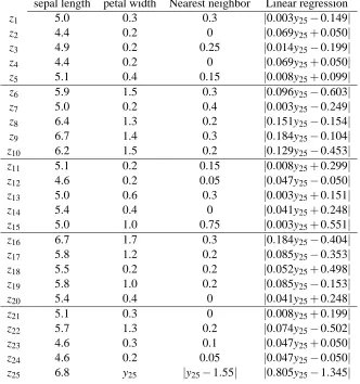
4.3.1 EXAMPLE: CLASSIFYINGIRISFLOWERS

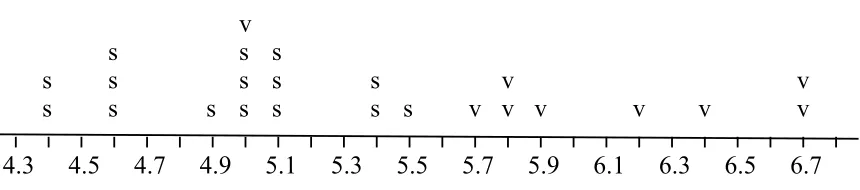
In 1936, R. A. Fisher used discriminant analysis to distinguish different species of iris on the basis of measurements of their flowers. The data he used included measurements by Edgar Anderson of flowers from 50 plants each of two species, iris setosa and iris versicolor. Two of the measurements, sepal length and petal width, are plotted in Figure 4.

To illustrate how the conformal algorithm can be used for classification, we have randomly chosen 25 of the 100 plants. The sepal lengths and species for the first 24 of them are listed in Table 2 and plotted in Figure 5. The 25th plant in the sample has sepal length 6.8. On the basis of this information, would you classify it as setosa or versicolor, and how confident would you be in the classification? Because 6.8 is the longest sepal in the sample, nearly any reasonable method will classify the plant as versicolor, and this is in fact the correct answer. But the appropriate level of confidence is not so obvious.

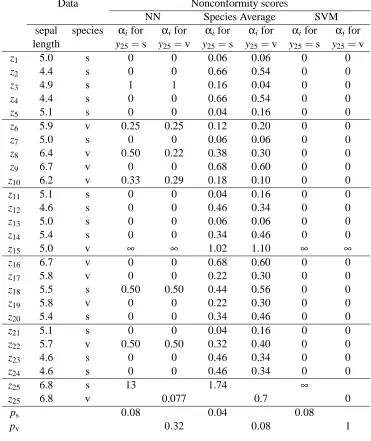
We calculate conformal prediction regions using three different nonconformity measures: one based on distance to the nearest neighbors, one based on distance to the species average, and one based on a support-vector machine. Because our evidence is relatively weak, we do not achieve the high precision with high confidence that can be achieved in many applications of machine learn-ing (see, for example, §4.5). But we get a clear view of the details of the calculations and the interpretation of the results.

Distance to the nearest neighbor belonging to each species. Here we use the nonconformity

measure (10). The fourth and fifth columns of Table 2 (labeled NN for nearest neighbor) give nonconformity scoresαiobtained with y25=s and y25=v, respectively. In both cases, these scores are given by

αi=A(*z1, . . . ,z25+\*zi+,zi)

=min{|xj−xi|: 1≤j≤25 & j6=i & yj=yi}

min{|xj−xi|: 1≤j≤25 & j6=i & yj6=yi}

, (19)

but for the fourth column z25= (6.8,s), while for the fifth column z25= (6.8,v).

If both the numerator and the denominator in (19) are equal to zero, we take the ratio also to be zero. This happens in the case of the first plant, for example. It has the same sepal length, 5.0, as the 7th and 13th plants, which are setosa, and the 15th plant, which is versicolor.

Step 3 of the conformal algorithm yields ps=0.08 and pv=0.32. Step 4 tells us that

• s is in the 1−εprediction region when 1−ε>0.92, and

• v is in the 1−εprediction region when 1−ε>0.68.

Here are prediction regions for a few levels ofε.

• Γ0.08_{={v}. With 92% confidence, we predict that y} 25=v.

• Γ0.05_{={s,v}. If we raise the confidence with which we want to predict y}

25 to 95%, the prediction is completely uninformative.

• Γ1/3₌/0_{. If we lower the confidence to 2/3, we get a prediction we know is false: y}

Data Nonconformity scores

NN Species Average SVM

sepal species αifor αifor αifor αifor αi for αifor

length y25=s y25=v y25=s y25=v y25=s y25=v

z1 5.0 s 0 0 0.06 0.06 0 0

z2 4.4 s 0 0 0.66 0.54 0 0

z3 4.9 s 1 1 0.16 0.04 0 0

z4 4.4 s 0 0 0.66 0.54 0 0

z5 5.1 s 0 0 0.04 0.16 0 0

z6 5.9 v 0.25 0.25 0.12 0.20 0 0

z7 5.0 s 0 0 0.06 0.06 0 0

z8 6.4 v 0.50 0.22 0.38 0.30 0 0

z9 6.7 v 0 0 0.68 0.60 0 0

z10 6.2 v 0.33 0.29 0.18 0.10 0 0

z11 5.1 s 0 0 0.04 0.16 0 0

z12 4.6 s 0 0 0.46 0.34 0 0

z13 5.0 s 0 0 0.06 0.06 0 0

z14 5.4 s 0 0 0.34 0.46 0 0

z15 5.0 v ∞ ∞ 1.02 1.10 ∞ ∞

z16 6.7 v 0 0 0.68 0.60 0 0

z17 5.8 v 0 0 0.22 0.30 0 0

z18 5.5 s 0.50 0.50 0.44 0.56 0 0

z19 5.8 v 0 0 0.22 0.30 0 0

z20 5.4 s 0 0 0.34 0.46 0 0

z21 5.1 s 0 0 0.04 0.16 0 0

z22 5.7 v 0.50 0.50 0.32 0.40 0 0

z23 4.6 s 0 0 0.46 0.34 0 0

z24 4.6 s 0 0 0.46 0.34 0 0

z25 6.8 s 13 1.74 ∞

z25 6.8 v 0.077 0.7 0

ps 0.08 0.04 0.08

pv 0.32 0.08 1

Table 2: Conformal prediction of iris species from sepal length, using three different noncon-formity measures. The data used are sepal length and species for a random sample of 25 of the 100 plants measured by Edgar Anderson. The second column gives xi, the sepal

1

3 3

3

3

3

3

3

2

2

2

2

2

2

2

2

2

2

2

2

2

1

1

1

1

1

1

5

1

1

1

1

1

1

1

1

1

1

1 1

1

1

1

1

1

1

1

1

1

1

1

1

1

1

1

1

1

1

1

1

1

1

1

1

1

1

1

1

1

4

4.5

5

5.5

6

6.5

7

0

0.2

0.4

0.6

0.8

1

1.2

1.4

1.6

1.8

sepal length

petal width

Figure 4: Sepal length, petal width, and species for Edgar Anderson’s 100 flowers. The 50 iris setosa are clustered at the lower left, while the 50 iris versicolor are clustered at the upper right. The numbers indicate how many plants have exactly the same measurement; for example, there are 5 plants that have sepals 5 inches long and petals 0.2 inches wide. Petal width separates the two species perfectly; all 50 versicolor petals are 1 inch wide or wider, while all setosa petals are narrower than 1 inch. But there is substantial overlap in sepal length.

In fact, y25=v. Our 92% prediction is correct.

The fact that we are making a known-to-be-false prediction with 2/3 confidence is a signal that the 25th sepal length, 6.8, is unusual for either species. A close look at the nonconformity scores reveals that it is being perceived as unusual simply because 2/3 of the plants have other plants in the sample with exactly the same sepal length, whereas there is no other plant with the sepal length 6.8.

4.3

s

s

s

s

s

s

v

s

s

s

s

s

s

s

s

s

v

v

v

v

v

v

v

v

4.5

4.7

4.9

5.1

5.3

5.5

5.7

5.9

6.1

6.3

6.5

6.7

Figure 5: Sepal length and species for the first 24 plants in our random sample of size 25. Ex-cept for one versicolor with sepal length 5.0, the versicolor in this sample all have longer sepals than the setosa. This high degree of separation is an accident of the sampling.

to avoid overconfidence when the object xn is unusual, it is wise to report also the largestε for

whichΓεis empty. We call this the credibility of the prediction (Vovk et al., 2005, p. 96).3 In our example, the prediction that y25will be v has credibility of only 32%, indicating that the example is somewhat unusual for the method that produces the prediction—so unusual that the method has 68% confidence in a prediction of y25that we know is false before we observe y25(Γ0.68=/0). Distance to the average of each species. The nearest-neighbor nonconformity measure, because it considers only nearby sepal lengths, does not take full advantage of the fact that a versicolor flower typically has longer sepals than a setosa flower. We can expect to obtain a more efficient conformal predictor (one that produces smaller regions for a given level of confidence) if we use a nonconformity measure that takes account of average sepal length for the two species.

We use the nonconformity measure A defined by

A(B,(x,y)) =|xB∪*(x,y)+,y−x|, (20)

where xB,y denotes the average sepal length of all plants of species y in the bag B, and B∪*z+

denotes the bag obtained by adding z to B. To test y25=s, we consider the bag consisting of the 24 old examples together with(6.8,s), and we calculate the average sepal lengths for the two species in this bag: 5.06 for setosa and 6.02 for versicolor. Then we use (20) to calculate the nonconformity scores shown in the sixth column of Table 2:

αi= (

|5.06−xi| if yi=s |6.02−xi| if yi=v

for i=1, . . . ,25, where we take y25to be s. To test y25=v, we consider the bag consisting of the 24 old examples together with(6.8,v), and we calculate the average sepal lengths for the two species in this bag: 4.94 for setosa and 6.1 for versicolor. Then we use (20) to calculate the nonconformity scores shown in the seventh column of Table 2:

αi= (

|4.94−xi| if yi=s |6.1−xi| if yi=v

for i=1, . . . ,25, where we take y25to be v. We obtain ps=0.04 and pv=0.08, so that

• s is in the 1−εprediction region when 1−ε>0.96, and

• v is in the 1−εprediction region when 1−ε>0.92.

Here are the prediction regions for some different levels ofε.

• Γ0.04_{={v}. With 96% confidence, we predict that y} 25=v.

• Γ0.03_{={s,v}. If we raise the confidence with which we want to predict y}

25 to 97%, the prediction is completely uninformative.

• Γ0.08_{=/0. If we lower the confidence to 92%, we get a prediction we know is false: y} 25 will be in the empty set.

In this case, we predict y25 =v with confidence 96% but credibility only 8%. The credibility is lower with this nonconformity measure because it perceives 6.8 as being even more unusual than the nearest-neighbor measure did. It is unusually far from the average sepal lengths for both species.

A support-vector machine. As Vladimir Vapnik explains on pp. 408–410 of his Statistical

Learn-ing Theory (1998), support-vector machines grew out of the idea of separatLearn-ing two groups of ex-amples with a hyperplane in a way that makes as few mistakes as possible—that is, puts as few examples as possible on the wrong side. This idea springs to mind when we look at Figure 5. In this one-dimensional picture, a hyperplane is a point. We are tempted to separate the setosa from the versicolor with a point between 5.5 and 5.7.

Vapnik proposed to separate two groups not with a single hyperplane but with a band: two hyperplanes with few or no examples between them that separate the two groups as well as possible. Examples on the wrong side of both hyperplanes would be considered very strange; those between the hyperplanes would also be considered strange but less so. In our one-dimensional example, the obvious separating band is the interval from 5.5 to 5.7. The only strange example is the versicolor with sepal length 5.0.

Here is one way of making Vapnik’s idea into an algorithm for calculating nonconformity scores for all the examples in a bag*(x1,y1), . . .(xn,yn)+. First plot all the examples as in Figure 5. Then

find numbers a and b such that a≤b and the interval[a,b]separates the two groups with the fewest mistakes—that is, minimizes4

#{i|1≤i≤n,xi<b, and yi=v}+#{i|1≤i≤n,xi>a, and yi=s}.

There may be many intervals that minimize this count; choose one that is widest. Then give the ith example the score

αi=  



∞ if yi=v and xi<a or yi=s and b<xi

1 if yi=v and a≤xi<b or yi=s and a<xi≤b

0 if yi=v and b≤xi or yi=s and xi≤a.

When applied to the bags in Figure 6, this algorithm gives the circled examples the score∞and all the others the score 0. These scores are listed in the last two columns of Table 2.

4.3 s s s s s s v s s s s s s s

s s v v

v v v v v

v v

4.5 4.7 4.9 5.1 5.3 5.5 5.7 5.9 6.1 6.3 6.5 6.7 4.3 s s s s s s v s s s s s s s

s s v s

v

v v v v

v v

4.5 4.7 4.9 5.1 5.3 5.5 5.7 5.9 6.1 6.3 6.5 6.7 4.3 s s s s s s v s s s s s s s

s s v v

v v v v

v v

4.5 4.7 4.9 5.1 5.3 5.5 5.7 5.9 6.1 6.3 6.5 6.7 The bag containing the 24 old examples

The bag of 25 examples, assuming the new example issetosa

The bag of 25 examples, assuming the new example isversicolor

Figure 6: Separation for three bags. In each case, the separating band is the interval[5.5,5.7]. Examples on the wrong side of the interval are considered strange and are circled.

As we see from the table, the resulting p-values are ps=0.08 and pv=1. So this time we obtain 92% confidence in y25=v, with 100% credibility.

The algorithm just described is too complex to implement when there are thousands of exam-ples. For this reason, Vapnik and his collaborators proposed instead a quadratic minimization that balances the width of the separating band against the number and size of the mistakes it makes. Support-vector machines of this type have been widely used. They usually solve the dual opti-mization problem, and the Lagrange multipliers they calculate can serve as nonconformity scores. Implementations sometimes fail to treat the old examples symmetrically because they make var-ious uses of the order in which examples are presented, but this difficulty can be overcome by a preliminary randomization (Vovk et al., 2005, p. 58).

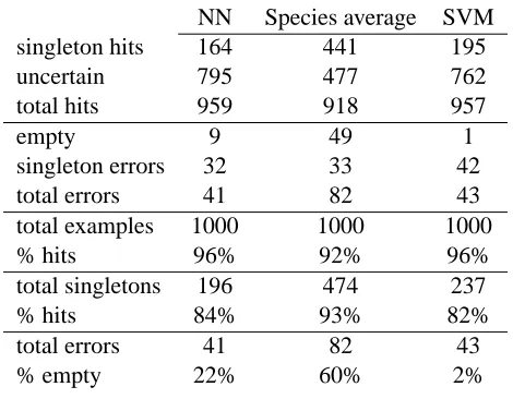
A systematic comparison. The random sample of 25 plants we have considered is odd in two

NN Species average SVM

singleton hits 164 441 195

uncertain 795 477 762

total hits 959 918 957

empty 9 49 1

singleton errors 32 33 42

total errors 41 82 43

total examples 1000 1000 1000

% hits 96% 92% 96%

total singletons 196 474 237

% hits 84% 93% 82%

total errors 41 82 43

% empty 22% 60% 2%

Table 3: Performance of 92% prediction regions based on three nonconformity measures. For each nonconformity measure, we have found 1,000 prediction regions at the 92% level, using each time a different random sample of 25 from Anderson’s 100 flowers. The “un-certain” regions are those equal to the whole label space, Y={s,v}.

in sepal length, and (2) the flower whose species we are trying to predict has a sepal that is unusually long for either species.

In order to get a fuller picture of how the three nonconformity measures perform in general on the iris data, we have applied each of them to 1,000 different samples of size 25 selected from the population of Anderson’s 100 plants. The results are shown in Table 3.

The 92% regions based on the species average were correct about 92% of the time (918 times out of 1000), as advertised. The regions based on the other two measures were correct more often, about 96% of the time. The reason for this difference is visible in Table 2; the nonconformity scores based on the species average take a greater variety of values and therefore produce ties less often. The regions based on the species averages are also more efficient (smaller); 441 of its hits were informative, as opposed to fewer than 200 for each of the other two nonconformity measures. This efficiency also shows up in more empty regions among the errors. The species average produced an empty 92% prediction region for the random sample used in Table 2, and Table 3 shows that this happens 5% of the time.

As a practical matter, the uncertain prediction regions (Γ0.08 _{={s,v}) and the empty ones} (Γ0.08=/0) are equally uninformative. The only errors that mislead are the singletons that are wrong, and the three methods all produce these at about the same rate—3 or 4%.

4.3.2 EXAMPLE: PREDICTINGPETALWIDTH FROMSEPALLENGTH