An
`
∞Eigenvector Perturbation Bound and Its Application
to Robust Covariance Estimation
Jianqing Fan [email protected]
Weichen Wang [email protected]
Yiqiao Zhong [email protected]
Department of Operations Research and Financial Engineering Princeton University
Princeton, NJ 08544, USA
Editor:Nicolai Meinshausen
Abstract
In statistics and machine learning, we are interested in the eigenvectors (or singular vec-tors) of certain matrices (e.g. covariance matrices, data matrices, etc). However, those matrices are usually perturbed by noises or statistical errors, either from random sampling or structural patterns. The Davis-Kahan sinθ theorem is often used to bound the differ-ence between the eigenvectors of a matrixAand those of a perturbed matrixAe=A+E,
in terms of `2 norm. In this paper, we prove that when A is a low-rank and incoherent matrix, the `∞ norm perturbation bound of singular vectors (or eigenvectors in the
sym-metric case) is smaller by a factor of√d1or √
d2for left and right vectors, whered1andd2 are the matrix dimensions. The power of this new perturbation result is shown in robust covariance estimation, particularly when random variables have heavy tails. There, we pro-pose new robust covariance estimators and establish their asymptotic properties using the newly developed perturbation bound. Our theoretical results are verified through extensive numerical experiments.
Keywords: Matrix perturbation theory, Incoherence, Low-rank matrices, Sparsity, Ap-proximate factor model
1. Introduction
The perturbation of matrix eigenvectors (or singular vectors) has been well studied in matrix perturbation theory (Wedin, 1972; Stewart, 1990). The best known result of eigenvector perturbation is the classic Davis-Kahan theorem (Davis and Kahan, 1970). It originally emerged as a powerful tool in numerical analysis, but soon found its widespread use in other fields, such as statistics and machine learning. Its popularity continues to surge in recent years, which is largely attributed to the omnipresent data analysis, where it is a common practice, for example, to employ PCA (Jolliffe, 2002) for dimension reduction, feature extraction, and data visualization.
The eigenvectors of matrices are closely related to the underlying structure in a variety of problems. For instance, principal components often capture most information of data and extract the latent factors that drive the correlation structure of the data (Bartholomew et al., 2011); in classical multidimensional scaling (MDS), the centered squared distance matrix encodes the coordinates of data points embedded in a low dimensional subspace
c
(Borg and Groenen, 2005); and in clustering and network analysis, spectral algorithms are used to reveal clusters and community structure (Ng et al., 2002; Rohe et al., 2011). In those problems, the low dimensional structure that we want to recover, is often ‘perturbed’ by observation uncertainty or statistical errors. Besides, there might be a sparse pattern corrupting the low dimensional structure, as in approximate factor models (Chamberlain et al., 1983; Stock and Watson, 2002) and robust PCA (De La Torre and Black, 2003; Cand`es et al., 2011).
A general way to study these problems is to consider
e
A=A+S+N, (1)
where A is a low rank matrix, S is a sparse matrix, and N is a random matrix regarded as random noise or estimation error, all of which have the same sized1×d2. Usually A is regarded as the ‘signal’ matrix we are primarily interested in,Sis some sparse contamination whose effect we want to separate fromA, andN is the noise (or estimation error in covariance matrix estimation).
The decomposition (1) forms the core of a flourishing literature on robust PCA (Chan-drasekaran et al., 2011; Cand`es et al., 2011), structured covariance estimation (Fan et al., 2008, 2013), multivariate regression (Yuan et al., 2007) and so on. Among these works, a standard condition onAis matrix incoherence (Cand`es et al., 2011). Let the singular value decomposition be
A=UΣVT =
r
X
i=1
σiuiviT, (2)
wherer is the rank of A, the singular values are σ1 ≥σ2 ≥. . .≥σr >0, and the matrices
U = [u1, . . . , ur] ∈ Rd1×r, V = [v1, . . . , vr] ∈ Rd2×r consist of the singular vectors. The
coherencesµ(U), µ(V) are defined as
µ(U) = d1
r maxi
r
X
j=1
Uij2, µ(V) = d2
r maxi
r
X
j=1
Vij2, (3)
where Uij and Vij are the (i, j) entry of U and V, respectively. It is usually expected that
µ0 := max{µ(U), µ(V)} is not too large, which means the singular vectors ui and vi are
incoherent with the standard basis. This incoherence condition (3) is necessary for us to separate the sparse component S from the low rank componentA; otherwiseA and S are not identifiable. Note that we do not need any incoherence condition on U VT, which is different from Cand`es et al. (2011) and is arguably unnecessary (Chen, 2015).
Now we denote the eigengap γ0 = min{σi−σi+1 : i = 1, . . . , r} where σr+1 := 0 for notational convenience. Also we let E = S +N, and view it as a perturbation matrix to the matrix A in (1). To quantify the perturbation, we define a rescaled measure as
τ0 := max{ p
d2/d1kEk1, p
d1/d2kEk∞}, where
kEk1 = max
j d1 X
i=1
|Eij|, kEk∞= max i
d2 X
j=1
which are commonly used norms gauging sparsity (Bickel and Levina, 2008). They are also operator norms in suitable spaces (see Section 2). The rescaled norms pd2/d1kEk1 andpd1/d2kEk∞are comparable to the spectral normkEk2 := maxkuk2=1kEuk2 in many
cases; for example, whenE is an all-one matrix,pd2/d1kEk1 = p
d1/d2kEk∞=kEk2. Suppose the perturbed matrixAealso has the singular value decomposition:
e
A=
d1∧d2 X
i=1 e
σiueive
T
i , (5)
where σei are nonnegative and in the decreasing order, and the notation ∧ meansa∧b =
min{a, b}. DenoteUe = [eu1, . . . ,uer], V = [ev1, . . . ,ver], which are counterparts of toprsingular
vectors ofA.
We will present an`∞matrix perturbation result that boundskeui−uik∞andkevi−vik∞
up to sign.1 This result is different from `2 bounds, Frobenius-norm bounds, or the sin Θ bounds, as the`∞ norm is not orthogonal invariant. The following theorem is a simplified
version of our main results in Section 2.
Theorem 1 LetAe=A+E and suppose the singular decomposition in (2) and (5). Denote
γ0 = min{σi−σi+1 :i = 1, . . . , r} where σr+1 := 0. Then there exists C(r, µ0) =O(r4µ20) such that, if γ0 > C(r, µ0)τ0, up to sign,
max
1≤i≤rkeui−uik∞≤C(r, µ0)
τ0
γ0
√
d1
and max
1≤i≤rkevi−vik∞≤C(r, µ0)
τ0
γ0
√
d2
, (6)
where µ0 = max{µ(U), µ(V)} is the coherence given after (3) and τ0 := max{p
d2/d1kEk1, p
d1/d2kEk∞}.
When A is symmetric, τ0 = kEk∞ and the condition on the eigengap is simply γ0 >
C(r, µ0)kEk∞. The incoherence condition naturally holds for a variety of applications,
where the low rank structure emerges as a consequence of a few factors driving the data matrix. For example, in Fama-French factor models, the excess returns in a stock market are driven by a few common factors (Fama and French, 1993); in collaborative filtering, the ratings of users are mostly determined by a few common preferences (Rennie and Srebro, 2005); in video surveillance, A is associated with the stationary background across image frames (Oliver et al., 2000). We will have a detailed discussion in Section 2.3.
The eigenvector perturbation was studied by Davis and Kahan (1970), where Hermitian matrices were considered, and the results were extended by Wedin (1972) to general rect-angular matrices. To compare our result with these classical results, assumingγ0 ≥2kEk2, a combination of Wedin’s theorem and Mirsky’s inequality (Mirsky, 1960) (the counterpart of Weyl’s inequality for singular values) implies
max 1≤k≤r
kvk−evkk2∨ kuk−eukk2 ≤
2√2kEk2
γ0
. (7)
wherea∨b:= max{a, b}.
1. ‘Up to sign’ means we can appropriately choose an eigenvector or singular vectoruto be eitheruor−u
Yu et al. (2015) also proved a similar bound as in (7), and that result is more convenient to use. If we are interested in the `∞ bound but naively use the trivial inequalitykxk∞≤
kxk2, we would have a suboptimal boundO(kEk2/γ0) in many situations, especially in cases where kEk2 is comparable to kEk∞. Compared with (6), the bound is worse by a factor
of √d1 foruk and
√
d2 forvk. In other words, converting the`2 bound from Davis-Kahan theorem directly to the`∞bound does not give a sharp result in general, in the presence of
incoherent and low rank structure ofA. Actually, assumingkEk2is comparable withkEk∞,
for square matrices, our `∞ bound (6) matches the`2 bound (7) in terms of dimensionsd1 andd2. This is becausekxk2 ≤
√
nkxk∞for anyx∈Rn, so we expect to gain a factor
√
d1 or√d2 in those `∞ bounds. The intuition is that, when A has an incoherent and low-rank
structure, the perturbation of singular vectors is not concentrated on a few coordinates.
To understand how matrix incoherence helps, let us consider a simple example with no matrix incoherence, in which (7) is tight up to a constant. LetA=d(1,0, . . . ,0)T(1,0, . . . ,0) be a d-dimensional square matrix, and E = d(0,1/2,0, . . . ,0)T(1,0, . . . ,0) of the same size. It is apparent that γ0 = d, τ0 = d/2, and that v1 = (1,0, . . . ,0)T,ev1 =
(2/√5,1/√5,0, . . . ,0)T up to sign. Clearly, the perturbation kev1 −v1k∞ is not
vanish-ing as d tends to infinity in this example, and thus, there is no hope of a strong upper bound as in (6) without the incoherence condition.
The reason that the factor √d1 or
√
d2 comes into play in (7) is that, the error uk−uek
(and similarly for vk) spreads out evenly in d1 (or d2) coordinates, so that the `∞ error is
far smaller than the`2 error. This, of course, hinges on the incoherence condition, which in essence precludes eigenvectors from aligning with any coordinate.
Our result is very different from the sparse PCA literature, in which it is usually assumed that the leading eigenvectors are sparse. In Johnstone and Lu (2009), it is proved that there is a threshold for p/n (the ratio between the dimension and the sample size), above which PCA performs poorly, in the sense that hev1, v1i is approximately 0. This means that the principal component computed from the sample covariance matrix reveals nothing about the true eigenvector. In order to mitigate this issue, in Johnstone and Lu (2009) and subsequent papers (Vu and Lei, 2013; Ma, 2013; Berthet and Rigollet, 2013), sparse leading eigenvectors are assumed. However, our result is different, in the sense that we require a stronger eigengap conditionγ0 > C(r, µ0)kEk∞(i.e. stronger signal), whereas in Johnstone
and Lu (2009), the eigengap of the leading eigenvectors is a constant times kEk2. This explains why it is plausible to have a strong uniform eigenvector perturbation bound in this paper.
We will illustrate the power of this perturbation result using robust covariance estimation as one application. In the approximate factor model, the true covariance matrix admits a decomposition into a low rank partA and a sparse part S. Such models have been widely applied in finance, economics, genomics, and health to explore correlation structure.
Here are a few notations in this paper. For a generic d1 by d2 matrix, the matrix max-norm is denoted askMkmax= maxi,j|Mij|. The matrix operator norm induced by vector`p
norm iskMkp = supkxkp=1kM xkp for 1≤p≤ ∞. In particular,kMk1 = maxj
Pd1
i=1|Mij|;
kMk∞= maxiPjd=12 |Mij|; and k · kdenotes the spectral norm, or the matrix 2-normk · k2 for simplicity. We use σj(M) to denote the jth largest singular value. For a symmetric
matrix M, denote λj(M) as its jth largest eigenvalue. If M is a positive definite matrix,
thenM1/2 is the square root of M, andM−1/2 is the square root of M−1.
2. The `∞ perturbation results
2.1 Symmetric matrices
First, we study `∞ perturbation for symmetric matrices (so d1 = d2). The approach we study symmetric matrices will be useful to analyze asymmetric matrices, because we can always augment ad1×d2 rectangular matrix into a (d1+d2)×(d1+d2) symmetric matrix, and transfer the study of singular vectors to the eigenvectors of the augmented matrix. This augmentation is calledHermitian dilation. (Tropp, 2012; Paulsen, 2002)
Suppose thatA∈Rd×dis and-dimensional symmetric matrix. The perturbation matrix
E ∈Rd×d is also d-dimensional and symmetric. Let the perturbed matrix be Ae:=A+E.
Suppose the spectral decomposition ofA is given by
A= [V, V⊥]
Λ1 0 0 Λ2
[V, V⊥]T = r
X
i=1
λiviviT +
X
i>r
λivivTi , (8)
where Λ1 = diag{λ1, . . . , λr}, Λ2 = diag{λr+1, . . . , λn}, and where|λ1| ≥ |λ2| ≥. . .≥ |λn|.
Note the best rank-r approximation ofA under the Frobenius norm isAr:=Pi≤rλivivTi .2
Analogously, the spectral decomposition ofAeis
e
A=
r
X
i=1 e
λiveive
T i +
X
i>r
e
λieviev
T i ,
and write Ve = [ev1, . . . ,evr]∈Rd×r, where |λe1| ≥ |eλ2| ≥ . . .≥ |λen|. Recall that kEk∞ given
by (4) is an operator norm in the `∞ space, in the sense that kEk∞ = supkuk∞≤1kEuk∞.
This norm is the natural counterpart of the spectral norm kEk2 := supkuk2≤1kEuk2. We will use notations O(·) and Ω(·) to hide absolute constants.3 The next theorem bounds the perturbation of eigenspaces up to a rotation.
Theorem 2 Suppose |λr| −ε = Ω(r3µ2kEk∞), where ε = kA−Ark∞, which is the
ap-proximation error measured under the matrix∞-norm and µ=µ(V) is the coherence of V
2. This is a consequence of Wielandt-Hoffman theorem.
3. We writea=O(b) if there is a constantC >0 such that a < Cb; anda= Ω(b) if there is a constant
defined in (3). Then, there exists an orthogonal matrix R∈Rr×r such that
kV Re −Vkmax=O
r5/2µ2kEk∞
(|λr| −ε)
√
d
!
.
This result involves an unspecified rotationR, due to the possible presence of multiplicity of eigenvalues. In the case where λ1 =· · · = λr >0, the individual eigenvectors of V are
only identifiable up to rotation. However, assuming an eigengap (similar to Davis-Kahan theorem), we are able to bound the perturbation of individual eigenvectors (up to sign).
Theorem 3 Assume the conditions in Theorem 2. In addition, suppose δ satisfies δ >
kEk2, and for any i∈[r], the interval[λi−δ, λi+δ]does not contain any eigenvalues of A
other than λi. Then, up to sign,
max
i∈[r]
kevi−vik∞=kVe −Vkmax=O
r4µ2kEk∞
(|λr| −ε)
√
d+
r3/2µ1/2kEk2
δ√d
!
.
To understand the above two theorems, let us consider the case where A has exactly rank r (i.e., ε = 0), and r and µ are not large (say, bounded by a constant). Theorem 2 gives a uniform entrywise bound O(kEk∞/|λr|
√
d) on the eigenvector perturbation. As a comparison, the Davis–Kahan sin Θ theorem (Davis and Kahan, 1970) gives a bound
O(kEk2/|λr|) onkV Re −Vk2 with suitably chosen rotationR.4 This is an order of
√
dlarger than the bound given in Theorem 2 when kEk∞ is of the same order as kEk2. Thus, in scenarios wherekEk2is comparable tokEk∞, this is a refinement of Davis-Kahan theorem,
because the max-norm bound in Theorem 2 provides an entry-wise control of perturbation. AlthoughkEk∞≥ kEk2,5there are many settings where the two quantities are comparable; for example, ifE has a submatrix whose entries are identical and has zero entries otherwise, thenkEk∞=kEk2.
Theorem 3 provides the perturbation of individual eigenvectors, under a usual eigengap assumption. Whenr andµare not large, we incur an additional termO(kEk2/δ
√
d) in the bound. This is understandable, sincekevi−vik2 is typicallyO(kEk2/δ).
When the rank ofAis not exactlyr, we require that|λr|is larger than the approximation
errorkA−Ark∞. It is important to state that this assumption is more restricted than the
eigengap assumption in the Davis-Kahan theorem, sincekA−Ark∞≥ kA−Ark2=|λr+1|. However, different from the matrix max-norm, the spectral normk · k2 only depends on the eigenvalues of a matrix, so it is natural to expect`2 perturbation bounds that only involve
λr and λr+1. It is not clear whether we should expect an `∞ bound that involves λr+1 instead ofε. More discussions can be found in Section 5.
We do not pursue the optimal bound in terms of r and µ(V) in this paper, as the two quantities are not large in many applications, and the current proof is already complicated.
4. To see how the Davis-Kahan sin Θ theorem relates to this form, we can use the identityksin Θ(V , Ve )k2= kVeVeT−V VTk2 (Stewart, 1990), and the (easily verifiable) inequality 2 minRkV Re −Vk2 ≥ kVeVeT−
V VTk2≥minRkV Re −Vk2 whereRis an orthogonal matrix.
2.2 Rectangular matrices
Now we establish`∞perturbation bounds for general rectangular matrices. The results here
are more general than those in Section 1, and in particular, we allow the matrix Ato be of approximate low rank. Suppose that bothA and E ared1×d2 matrices, and Ae:=A+E.
The rank of A is at mostd1∧d2 (wherea∧b= min{a, b}). Suppose an integer r satisfies
r≤rank(A). Let the singular value decomposition ofA be
A=
r
X
i=1
σiuivTi + d1∧d2
X
i=r+1
σiuiviT,
where the singular values are ordered asσ1 ≥σ2 ≥. . . ≥σd1∧d2 ≥0, and the unit vectors
u1, . . . , ud1∧d2 (or unit vectors v1, . . . , vd1∧d2) are orthogonal to each other. We denote
U = [u1, . . . , ur] ∈ Rd1×r and V = [v1, . . . , vr] ∈ Rd2×r. Analogously, the singular value
decomposition ofAeis
e
A=
r
X
i=1 e
σiueiev
T i +
d1∧d2 X
i=r+1 e
σiueive
T i ,
where σe1 ≥ . . . ≥ σed1∧d2. Similarly, columns of Ue = [eu1, . . . ,uer] ∈ R
d1×r and e
V =
[ev1, . . . ,evr]∈R
d2×r are orthonormal.
Define µ0 = max{µ(V), µ(U)}, where µ(U) (resp. µ(V)) is the coherence of U (resp.
V). This µ0 will appear in the statement of our results, as it controls both the structure of left and right singular spaces. When, specially, A is a symmetric matrix, the spectral decomposition of A is also the singular value decomposition (up to sign), and thus µ0 coincides withµ defined in Section 2.1.
Recall the definition of matrix∞-norm and 1-norm of a rectangular matrix (4). Similar to the matrix ∞-norm, k · k1 is an operator norm in the `1 space. An obvious relationship between matrix ∞-norm and 1-norm is kEk∞ = kETk1. Note that the matrix ∞-norm and 1-norm have different number of summands in their definitions, so we are motivated to consider τ0 := max{
p
d1/d2kEk∞,
p
d2/d1kEk1} to balance the dimensionsd1 and d2. Let Ar = Pi≤rσiuiviT be the best rank-r approximation of A under the Frobenius
norm, and let ε0 = p
d1/d2kA−Ark∞∨
p
d2/d1kA−Ark1, which also balances the two dimensions. Note that in the special case where A is symmetric, this approximation error
ε0 is identical to ε defined in Section 2.1. The next theorem bounds the perturbation of singular spaces.
Theorem 4 Suppose that δ0 −ε0 = Ω(r3µ20τ0). Then, there exists orthogonal matrices
RU, RV ∈Rr×r such that,
kU Re U−Ukmax=O
r5/2µ2 0τ0 (σr−0)
√
d1
, kV Re V −Vkmax=O
r5/2µ2 0τ0 (σr−0)
√
d2
.
Theorem 5 Suppose the same assumptions in Theorem 4 hold. In addition, suppose δ0 satisfies δ0 >kEk2, and for any i∈[r], the interval[σi−δ0, σi+δ0] does not contain any eigenvalues of A other than σi. Then, up to sign,
max
i∈[r]
kuei−uik∞=O
r4µ2 0τ0 (σr−ε0)
√
d1 +r
3/2µ1/2 0 kEk2
δ0
√
d1
, (9)
max
i∈[r]
kevi−vik∞=O
r4µ2 0τ0 (σr−ε0)
√
d2 +r
3/2µ1/2 0 kEk2
δ0
√
d2
. (10)
As mentioned in the beginning of this section, we will use dilation to augment alld1×d2 matrices into symmetric ones with size d1+d2. In order to balance the possibly different scales ofd1 andd2, we consider a weighted max-norm. This idea will be further illustrated in Section 5.
2.3 Examples: which matrices have such structure?
In many problems, low-rank structure naturally arises due to the impact of pervasive latent factors that influence most observed data. Since observations are imperfect, the low-rank structure is often ‘perturbed’ by an additional sparse structure, gross errors, measurement noises, or the idiosyncratic components that can not be captured by the latent factors. We give some motivating examples with such structure.
Panel data in stock markets. Consider the excess returns from a stock market over a period of time. The driving factors in the market are reflected in the covariance matrix as a low rank component A. The residual covariance of the idiosyncratic components is often modeled by a sparse component S. Statistical analysis including PCA is usually conducted based on the estimated covariance matrix Ae=Σ, which is perturbed from theb
true covariance Σ =A+S by the estimation error N (Stock and Watson, 2002; Fan et al., 2013). In Section 3.1, we will develop a robust estimation method in the presence of heavy-tailed return data.
Video surveillance. In image processing and computer vision, it is often desired to separate moving objects from static background before further modeling and analysis (Oliver et al., 2000; Hu et al., 2004). The static background corresponds to the low rank component
A in the data matrix, which is a collection of video frames, each consisting of many pixels represented as a long vector in the data matrix. Moving objects and noise correspond to the sparse matrix S and noise matrix N. Since the background is global information and reflected by many pixels of a frame, it is natural for the incoherence condition to hold.
Wireless sensor network localization. In wireless sensor networks, we are usually inter-ested in determining the location of sensor nodes with unknown position based on a few (noisy) measurements between neighboring nodes (Doherty et al., 2001; Biswas and Ye, 2004). Let X be an r by n matrix such that each column xi gives the coordinates of each
node in a plane (r = 2) or a space (r = 3). Assume the center of the sensors has been relocated at origin. Then the low rank matrix A=XTX, encoding the true distance
errors. Suppose that each node is a random point uniformly distributed in a rectangular region. It is not difficult to see that with high probability, the top r eigenvalues of XTX
and their eigengap scales with the number of sensorsnand the leading eigenvectors have a bounded coherence.
In our theorems, we require that the coherence µ is not too large. This is a natural structural condition associated with the low rank matrices. Consider the following very simple example: if the eigenvectors v1, . . . , vr of the low rank matrix A are uniform unit
vectors in a sphere, then with high probability, maxikvik∞=O(
√
logn), which impliesµ=
O(logn). An intuitive way to understand the incoherence structure is that no coordinates
of v1 (or v2, . . . vr) are dominant. In other words, the eigenvectors are not concentrated on
a few coordinates.
In all our examples, the incoherence structure is natural. The factor model satisfies such structure, which will be discussed in Section 3. In the video surveillance example, ideally, when the images are static, A is a rank one matrixx1T. Since usually a majority of pixels (coordinates ofx) help to display an image, the vectorx often has dense coordinates with comparable magnitude, so A also has an incoherence structure in this example. Similarly, in the sensor localization example, the coordinates of all sensor nodes are comparable in magnitude, so the low rank matrix A formed by XTX also has the desired incoherence
structure.
2.4 Other perturbation results
Although the eigenvector perturbation theory is well studied in numerical analysis, there is a renewed interest among statistics and machine learning communities recently, due to the wide applicability of PCA and other eigenvector-based methods. In Cai and Zhang (2016); Yu et al. (2015), they obtained variants or improvements of Davis-Kahan theorem (or Wedin’s theorem), which are user-friendly in the statistical contexts. These results assume the perturbation is deterministic, which is the same as Davis-Kahan theorem and Wedin’s theorem. In general, these results are sharp, even when the perturbation is random, as evidenced by the BBP transition (Baik et al., 2005).
However, these classical results can be suboptimal, when the perturbation is random and the smallest eigenvalue gapλ1−λ2 does not capture particular spectrum structure. For example, Vu (2011); O’Rourke et al. (2013) showed that with high probability, there are bounds sharper than the Wedin’s theorem, when the signal matrix is low-rank and satisfies certain eigenvalue conditions.
In this paper, our perturbation results are deterministic, thus the bound can be subop-timal when the perturbation is random with certain structure (e.g. the difference between sample covariance and population one for i.i.d. samples). However, the advantage of a deterministic result is that it is applicable to any random perturbation. This is especially useful when we cannot make strong random assumptions on the perturbation (e.g., the perturbation is an unknown sparse matrix). In Section 3, we will see examples of this type.
3. Application to robust covariance estimation
coher-enceµ(V) are bounded by a constant, though this assumption can be relaxed. We will use
C to represent a generic constant, and its value may change from line to line.
3.1 PCA in spiked covariance model
To initiate our discussions, we first consider sub-Gaussian random variables. Let X =
(X1, . . . , Xd) be a random d-dimensional vector with mean zero and covariance matrix
Σ =
r
X
i=1
λiviviT +σ2Id:= Σ1+ Σ2, (λ1 ≥. . .≥λr>0), (11)
andXbe annbydmatrix, whose rows are independently sampled from the same
distribu-tion. This is the spiked covariance model that has received intensive study in recent years. Let the empirical covariance matrix be Σ =b XTX/n. Viewing the empirical covariance
matrix as its population version plus an estimation error, we have the decomposition
b
Σ = Σ1+ Σ2+ 1
nX
T
X−Σ
,
which is a special case of the general decomposition in (1). Here, Σ2is the sparse component, and the estimation errorXTX/n−Σ is the noise component. Note thatv1, . . . , vrare just the
toprleading eigenvectors of Σ and we writeV = [v1, . . . , vr]. Assume the topreigenvectors
ofΣ are denoted byb bv1, . . . ,bvr. We want to find an`∞bound on the estimation errorvbi−vi
for all i∈[r].
When the dimensiondis comparable to or larger thann, it has been shown by Johnstone and Lu (2009) that the leading empirical eigenvectorvb1 is not a consistent estimate of the
true eigenvector v1, unless we assume larger eigenvalues. Indeed, we will impose more stringent conditions on λi’s in order to obtain good `∞ bounds.
Assuming the coherence µ(V) is bounded, we can easily see Var(Xj)≤σ2+Cλ1/dfor some constantC. It follows from the standard concentration result (e.g., Vershynin (2010)) that if rows ofXcontains i.i.d sub-Gaussian vectors and logd=O(n), then with probability
greater than 1−d−1,
k1
nX
T
X−Σkmax≤C σ2+
λ1
d
r
logd
n . (12)
To apply Theorem 3, we treat Σ1 as A and Σb −Σ1 as E. If the conditions in Theorem 3
are satisfied, we will obtain
max
1≤k≤rkbvk−vkk∞=O(kEk∞/(λr
√
d) +kEk2/(δ√d)). (13)
Note there are simple bounds onkEk∞ andkEk2:
kEk2≤ kEk∞≤σ2+dk
1
nX
T
X−Σkmax≤C
n
1 + dσ2+λ1
r
logd n
o
By assuming a strong uniform eigengap, the conditions in Theorem 3 are satisfied, and the bound in (13) can be simplified. Define the uniform eigengap as
γ= min{λi−λi+1: 1≤i≤r}, λr+1 := 0. Note thatγ ≤min{λr, δ}, so ifγ > C(1 + dσ2+λ1
p
logd/n), we have
max
1≤k≤rkbvk−vkk∞=OP
kEk∞
γ√d
=OP
1 + dσ2+λ1plogd/n
γ√d
,
In particular, whenλ1γ andγ max{1, σ2d p
logd/n}, we have
max
1≤k≤rkbvk−vkk∞=oP
1
√
d
.
The above analysis pertains to the structure of sample covariance matrix. In the following subsections, we will estimate the covariance matrix using more complicated robust proce-dure. Our perturbation theorems in Section 2 provide a fast and clean approach to obtain new results.
3.2 PCA for robust covariance estimation
The usefulness of Theorem 3 is more pronounced when the random variables are heavy-tailed. Consider again the covariance matrix Σ with structure (11). Instead of assuming sub-Gaussian distribution, we assume there exists a constantC >0 such that maxj≤dEXj4< C,
i.e. the fourth moments of the random variables are uniformly bounded.
Unlike sub-Gaussian variables, there is no concentration bound similar to (12) for the empirical covariance matrix. Fortunately, thanks to recent advances in robust statistics (e.g., Catoni (2012)), robust estimate of Σ with guaranteed concentration property becomes possible. We shall use the method proposed in Fan et al. (2017a). Motivated by the classical
M-estimator of Huber (1964), Fan et al. (2017a) proposed a robust estimator for each element ofΣ, by solving a Huber loss based minimization problemb
b
Σij = argminµ n
X
t=1
lα(XtiXtj−µ), (14)
wherelα is the Huber loss defined as
lα(x) =
(
2α|x| −α2, |x| ≥α,
x2, |x| ≤α.
The parameterα is suggested to be α=pnv2/log(−1) for ∈(0,1), wherev is assumed to satisfyv≥maxij
p
Var(XiXj). If log(−1)≤n/8, Fan et al. (2017a) showed
P|Σbij−Σij| ≤4v r
log(−1)
n
From this result, the next proposition is immediate by taking =d−3.
Proposition 1 Suppose that there is a constant C with maxj≤dEXj4 < C. Then with
probability greater than 1−d−1(1 +d−1), the robust estimate of covariance matrix with
α=p3nv2log(d) satisfies
kΣb−Σkmax≤4v r
3 logd
n ,
where v is a pre-determined parameter assumed to be no less than maxij
p
Var(XiXj).
This result relaxes the sub-Gaussianity assumption by robustifying the covariance esti-mate. It is apparent that the`∞ bound in the previous section is still valid in this case. To
be more specific, suppose µ(V) is bounded by a constant. Then, (13) holds for the PCA based on the robust covariance estimation. When λ1 γ and γ max{1, σ2d
p
logd/n}, we again have
max
1≤k≤rkvbk−vkk∞=OP
1 + dσ2+λ1plogd/n
γ√d
=oP
1
√
d
.
Note that an entrywise estimation error op(1/
√
d) necessarily implies consistency of the estimated eigenvectors, since we can easily convert an `∞ result into an `2 result. The minimum signal strength (or magnitude of leading eigenvalues) for such consistency is shown to beσ2d/nunder the sub-Gaussian assumption (Wang and Fan, 2017).
If the goal is simply to prove consistency ofbvk, the strategy of using our`∞perturbation
bounds is not optimal. However, there are also merits: our result is nonasymptotic; it holds for more general distributions (beyond sub-Gaussian distributions); and its entrywise bound gives stronger guarantee. Moreover, the`∞ perturbation bounds provide greater flexibility
for analysis, since it is straightforward to adapt analysis to problems with more complicated structure. For example, the above discussion can be easily extended to a general Σ2 with bounded kΣ2k∞ rather than a diagonal matrix.
3.3 Robust covariance estimation via factor models
In this subsection, we will apply Theorem 3 to robust large covariance matrix estimation for approximate factor models in econometrics. With this theorem, we are able to extend the data distribution in factor analysis beyond exponentially decayed distributions considered by Fan et al. (2013), to include heavy-tailed distributions.
Suppose the observationyit, say, the excess return at daytfor stocki, admits a
decom-position
yit=bTi ft+uit, i≤d, t≤n, (15)
wherebi∈Rris the unknown but fixed loading vector,ft∈Rrdenotes the unobserved factor
vector at time t, and uit’s represent the idiosyncratic noises. Let yt = (y1t, . . . , ydt)T and
ut = (u1t, . . . , udt)T so that yt =Bft+ut, where B = (b1, . . . , bd)T ∈Rd×r. Suppose that ft and ut are uncorrelated and centered random vectors, with bounded fourth moments,
i.e., the fourth moments of all entries of ft and ut are bounded by some constant. We
dependence as in Fan et al. (2013). From (15), we can decompose Σ = Cov(yt) into a low
rank component and a residual component:
Σ =BBT + Σu, (16)
where Σu := Cov(ut). To circumvent the identifiability issue common in latent variable
models, here we also assume, without loss of generality, Cov(ft) = Ir and that BTB is a
diagonal matrix, since rotatingB will not affect the above decomposition (16).
We will need two major assumptions for our analysis: (1) the factors are pervasive in the sense of Definition 2, and (2) there is a constantC >0 such that kΣ−u1k2,kΣuk2 ≤C, which are standard assumptions in the factor model literature. The pervasive assumption is reasonable in financial applications, since the factors have impacts on a large fraction of the outcomes (Chamberlain et al., 1983; Bai, 2003). If the factor loadings {bi}di=1 are regarded as random realizations from a bounded random vector, the assumption holds (Fan et al., 2013).
Definition 2 In the factor model (15), the factors are called pervasive if there is a constant
C >0 such that kBkmax≤C and the eigenvalues of the r by r matrixBTB/dare distinct
and bounded away from zero and infinity.
Let {λi, vi}ri=1 be the topr eigenvalues and eigenvectors of Σ, and similarly, {λi, vi}ri=1 forBBT. In the following proposition, we show that pervasiveness is naturally connected to the incoherence structure. This connects the econometrics and machine learning literature and provide a good interpretation on the concept of the incoherence. Its proof can be found in the appendix.
Proposition 3 Suppose there exists a constantC >0 such thatkΣuk ≤C. The factors ft
are pervasive if and only if the coherence µ(V) for V = (v1, . . . , vr)∈ Rd×r is bounded by
some constant, and λi =λi(Σ)d for i≤r so thatmin1≤i6=j≤r|λi−λj|/λj >0.
Our goal is to obtain a good covariance matrix estimator by exploiting the structure (16). Our strategy is to use a generalization of the principal orthogonal complement thresholding (POET) method proposed in Fan et al. (2013). The generic POET procedure encompasses three steps:
(1) Given three pilot estimatorsΣb,Λ = diag(b bλ1, . . . ,bλr),Vb = (bv1, . . . ,bvr) respectively for
true covariance Σ, leading eigenvalues Λ = diag(λ1, . . . , λr) and leading eigenvectors
V = (v1, . . . , vr), compute the principal orthogonal complement Σbu:
b
Σu =Σb−VbΛbVbT. (17)
(2) Apply the correlation thresholding to Σbu to obtain thresholded estimate Σb>u defined
as follows:
b
Σ>u,ij =
( b
Σu,ij, i=j
sij(Σbu,ij)I(|Σbu,ij| ≥τij), i6=j
, (18)
wheresij(·) is the generalized shrinkage function (Antoniadis and Fan, 2001; Rothman
et al., 2009) and τij = τ(ˆσu,iiσˆu,jj)1/2 is an entry-dependent threshold. τ will be
(3) Construct the final estimatorΣb>=VbΛbVbT +Σb>u.
The key feature in the above procedure lies in the flexibility of choosing the pilot estima-tors in the first step. We will chooseΣ according to data generating distribution. Typicallyb
we can use ˆλi,ˆvi for i ≤r as the eigenvalues/vectors of Σ. However, ˆb Λ and ˆV in general
do not have to come from the spectral information ofΣ and can be obtained separately viab
different methods.
To guide the selection of proper pilot estimators, Fan et al. (2017+) provided a high level sufficient condition for this simple procedure to be effective, and its performance is gauged, in part, through the sparsity level of Σu, defined as md := maxi≤d
P
j≤d|Σu,ij|q.
When q = 0, md corresponds to the maximum number of nonzero elements in each row of
Σu. For completeness, we present the theorem given by Fan et al. (2017+) in the following.
Theorem 6 Let wn =
p
logd/n + 1/√d. Suppose there exists C > 0 such that
kΣ−u1k,kΣuk ≤C and we have pilot estimators Σb,Λb,Vb satisfying
kΣb−Σkmax=O( p
logd/n), (19)
|bλi/λi−1|=O( p
logd/n), (20)
kbvi−vik∞=O(wn/
√
d). (21)
Under the pervasiveness condition of the factor model (15), withτ wn, ifmdw1n−q =o(1),
the following rates of convergence hold with the generic POET procedure:
kΣb>u −Σuk2 =O
mdwn1−q
=k(Σb>u)−1−Σu−1k2, (22) and
kΣb>−Σkmax=O
wn
,
kΣb>−ΣkΣ =O
√
dlogd
n +mdw
1−q n
,
k(Σb>)−1−Σ−1k2=O
mdw1n−q
,
(23)
where kAkΣ=d−1/2kΣ−1/2AΣ−1/2kF is the relative Frobenius norm.
We remark that the additional term 1/√dinwn, is due to the estimation of unobservable
factors and is negligible when the dimensional dis high. The optimality of the above rates of convergence is discussed in details in Fan et al. (2017+). Theorem 6 reveals a profound deterministic connection between the estimation error bound of the pilot estimators with the rate of convergences of the POET output estimators. Notice that the eigenvector estimation error is under the`∞ norm, for which our`∞ perturbation bounds will prove to be useful.
In this subsection, since we assume only bounded fourth moments, we chooseΣ to be theb
robust estimate of covariance matrix Σ defined in (14). We now invoke our `∞ bounds to
Let us decompose Σ into a form such that Theorem 3 can be invoked:b
b
Σ =
r
X
i=1
λivivTi + Σu+ (Σb−Σ),
whereΣ is viewed asb Ae, the low-rank part Pr
i=1λivivTi , which is alsoBBT, is viewed asA,
and the remaining terms are treated as E. The following results follow immediately.
Proposition 4 Assume that there is a constant C >0 such that kΣuk ≤C. If the factors
are pervasive, then with probability greater than1−d−1, we have (19) – (21) hold withbλi,bvi as the leading eigenvalues/vectors of Σb for i≤r. In addition, (22) and (23) hold.
The inequality (19) follows directly from Proposition 1 under the assumption of bounded fourth moments. It is also easily verifiable that (20), (21) follow from (19) by Weyl’s inequality and Theorem 3 (noting that kΣuk∞ ≤
√
dkΣuk). See Section 3.2 for more
details.
Note that in the case of sub-Gaussian variables, sample covariance matrix and its leading eigenvalues/vectors will also serve the same purpose due to (12) and Theorem 3 as discussed in Section 3.1.
We have seen that the `∞ perturbation bounds are useful in robust covariance
estima-tion, and particularly, they resolve a theoretical difficulty in the generic POET procedure for factor model based covariance matrix estimation.
4. Simulations
4.1 Simulation: the perturbation result
In this subsection, we implement numerical simulations to verify the perturbation bound in Theorem 3. We will show that the error behaves in the same way as indicated by our theoretical bound.
In the experiments, we let the matrix size d run from 200 to 2000 by an increment of 200. We fix the rank of A to be 3 (r = 3). To generate an incoherence low rank matrix, we sample a d×d random matrix with iid standard normal variables, perform singular value decomposition, and extract the first r right singular vectors v1, v2, . . . , vr.
Let V = (v1, . . . , vr) and D = diag(rγ,(r −1)γ, . . . , γ) where γ as before represents the
eigengap. Then, we set A=V DVT. By orthogonal invariance, vi is uniformly distributed
on the unit sphereSd−1. It is not hard to see that with probability 1−O(d−1), the coherence
of V µ(V) =O(√logd).
We consider two types of sparse perturbation matrices E: (a) construct a d×dmatrix
E0 by randomly selectingsentries for each row, and sampling a uniform number in [0, L] for each entry, and then symmetrize the perturbation matrix by settingE = (E0+E0T)/2; (b) pickρ∈(0,1), L0 >0, and letEij =L0ρ|i−j|. Note that in (b) we havekEk∞≤2L0/(1−ρ),
and thus we can choose suitable L0 and ρ to control the `∞ norm of E. This covariance
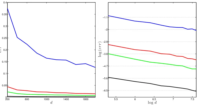
200 600 1000 1400 1800 0
0.05 0.1 0.15 0.2 0.25 0.3 0.35 0.4
d
e
r
r
5.5 6 6.5 7 7.5
−6.5 −5.6 −4.7 −3.8 −2.9 −2 −1.1
logd
lo
g
(
e
r
r
)
Figure 1: The left plot shows the perturbation error of eigenvectors against matrix size d
ranging from 200to 2000, with different eigengap γ. The right plot shows log(err) against log(d). The slope is around −0.5. Blue lines represent γ= 10; red lines γ = 50; green lines
γ = 100; and black lines γ = 500. We report the largest error over100 runs.
The perturbation of eigenvectors is measured by the element-wise error:
err:= max
1≤i≤rηimin∈{±1}
kηievi−vik∞,
where{evi}ri=1 are the eigenvectors of Ae=A+E in the descending order.
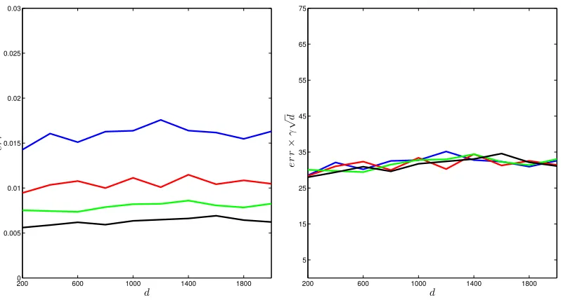
To investigate how the error depends onγ andd, we generateEaccording to mechanism (a) with s = 10, L = 3, and run simulations in different parameter configurations: (1) let the matrix size d range from 200 to 2000, and choose the eigengap γ in {10,50,100,500}
(Figure 1); (2) fix the productγ√dto be one of{2000,3000,4000,5000}, and let the matrix sizedrun from 200 to 2000 (Figure 2).
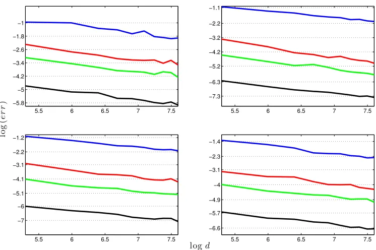
To find how the errors behave forEgenerated from different methods, we run simulations as in (1) but generate E differently. We construct E through mechanism (a) with L = 10, s= 3 and L = 0.6, s= 50, and also through mechanism (b) with L0 = 1.5, ρ= 0.9 and
L0 = 7.5, ρ= 0.5 (Figure 3). The parameters are chosen such that kEk∞ is about 30.
In Figure 1 – 3, we report the largest error based on 100 runs. Figure 1 shows that the error decreases asdincreases (the left plot); and moreover, the logarithm of the error is linear in log(d), with a slope−0.5, that is,err∝1/√d(the right plot). We can take the eigengap
γ into consideration and characterize the relationship in a more refined way. In Figure 2, it is clear that err almost falls on the same horizontal line for different configurations of
200 600 1000 1400 1800 0
0.005 0.01 0.015 0.02 0.025 0.03
d
e
r
r
200 600 1000 1400 1800
5 15 25 35 45 55 65 75
d
e
r
r
×
γ
√
d
Figure 2: The left plot shows the perturbation error of eigenvectors against matrix size d
ranging from 200 to 2000, when γ√d is kept fixed, with different values. The right plot shows the error multiplied by γ√d against d. Blue lines represent γ√d = 2000; red lines
γ√d= 3000; green lines γ√d= 4000; and black lines γ√d= 5000. We report the largest error over 100runs.
same regardless of how E is generated. These simulation results provide stark evidence supporting the `∞ perturbation bound in Theorem 3.
4.2 Simulation: robust covariance esitmation
We consider the performance of the generic POET procedure in robust covariance estimation in this subsection. Note that the procedure is flexible in employing any pilot estimators
b
Σ,Λb,Vb satisfying the conditions (19) – (21) respectively.
We implemented the robust procedure with four different initial trios: (1) the sample covarianceΣbSwith its leadingreigenvalues and eigenvectors asΛbS andVbS; (2) the Huber’s
robust estimator ΣbR given in (14) and its top r eigen-structure estimatorsΛbR and VbR; (3)
the marginal Kendall’s tau estimatorΣbK with its correspondingΛbK andVbK; (4) lastly, we
use the spatial Kendall’s tau estimator to estimate the leading eigenvectors instead of the marginal Kendall’ tau, soVbK in (3) is replaced withVeK. We need to briefly review the two
types of Kendall’s tau estimators here, and specifically give the formula for ΣbK and VeK.
Kendall’s tau correlation coefficient, for estimating pairwise comovement correlation, is defined as
ˆ
τjk :=
2
n(n−1)
X
t<t0
5.5 6 6.5 7 7.5 −5.8
−5 −4.2 −3.4 −2.6 −1.8 −1
5.5 6 6.5 7 7.5 −7.3
−6.3 −5.2 −4.2 −3.2 −2.2 −1.1
5.5 6 6.5 7 7.5 −7
−6 −5.1 −4.1 −3.1 −2.2 −1.2
5.5 6 6.5 7 7.5 −6.6
−5.7 −4.9 −4 −3.1 −2.3 −1.4
lo
g
(
e
r
r
)
logd
Figure 3: These plots show log(err) aginst log(d), with matrix size d ranging from 200 to 2000 and different eigengap γ. The perturbation E is generated from different ways. Top left: L = 10, s = 3; top right: L = 0.6, s = 50; bottom left: L0 = 1.5, ρ = 0.9; bottom right: L0 = 7.5, ρ= 0.5. The slopes are around −0.5. Blue lines represent γ = 10; red lines
γ = 50; green lines γ = 100; and black lines γ = 500. We report the largest error over100 runs.
Its population expectation is related to the Pearson correlation via the transform rjk =
sinπ2 E[ˆτjk]
for elliptical distributions (which are far too restrictive for high-dimensional
applications). Then ˆrjk = sin
π
2τˆjk
is a valid estimation for the Pearson correlation
rjk. Letting Rb = (ˆrjk) and Db = diag( q
b
ΣR
11, . . . , q
b
ΣR
dd) containing the robustly estimated
standard deviations, we define the marginal Kendall’s tau estimator as
b
ΣK =DbRbD .b (25)
In the above construction ofDb, we still use the robust variance estimates from ΣbR.
The spatial Kendall’s tau estimator is a second-order U-statstic, defined as
e
ΣK := 2
n(n−1)
X
t<t0
(yt−yt0)(yt−yt0)T
kyt−yt0k2 2
Then VeS is constructed by the top r eigenvectors of ΣeK. It has been shown by Fan
et al. (2017+) that under elliptical distribution, ΣbK and its top r eigenvalues ΛbK satisfy
(19) and (20) while VeS suffices to conclude (21). Hence Method (4) indeed provides good
initial estimators if data are from elliptical distribution. However, since ΣbK attains (19)
for elliptical distribution, by similar argument for deriving Proposition 4 based on our `∞
pertubation bound, VbK consisting of the leading eigenvectors of ΣbK is also valid for the
generic POET procedure. For more details about the two types of Kendall’s tau, we refer the readers to Fang et al. (1990); Choi and Marden (1998); Han and Liu (2014); Fan et al. (2017+) and references therein.
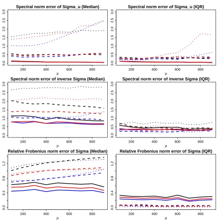
In summary, Method (1) is designed for the case of sub-Gaussian data; Method (3) and (4) work under the situation of elliptical distribution; while Method (2) is proposed in this paper for the general heavy-tailed case with bounded fourth moments without further distributional shape constraints.
We simulatednsamples of (ftT, uTt)T from two settings: (a) a multivariate t-distribution with covariance matrix diag{Ir,5Id} and various degrees of freedom (ν = 3 for very heavy
tail, ν = 5 for medium heavy tail and ν = ∞ for Gaussian tail), which is one example of the elliptical distribution (Fang et al., 1990); (b) an element-wise iid one-dimensional t distribution with the same covariance matrix and degrees of freedomν= 3,5 and∞, which is a non-elliptical heavy-tailed distribution.
Each row of coefficient matrix B is independently sampled from a standard normal distribution, so that with high probability, the pervasiveness condition holds withkBkmax=
O(√logd). The data is then generated byyt=Bft+utand the true population covariance
matrix is Σ =BBT + 5Id.
For d running from 200 to 900 and n = d/2, we calculated errors of the four robust estimators in different norms. The tuning for α in minimization (14) is discussed more throughly in Fan et al. (2017b). For the thresholding parameter, we used τ = 2plogd/n. The estimation errors are gauged in the following norms: kΣb>u −Σuk, k(Σb>)−1 −Σ−1k
and kΣb>−ΣkΣ as shown in Theorem 6. The two different settings are separately plotted
in Figures 4 and 5. The estimation errors of applying sample covariance matrix ΣbS in
Method (1) are used as the baseline for comparison. For example, if relative Frobenius norm is used to measure performance,k(Σb>)(k)−ΣkΣ/k(Σb>)(1)−ΣkΣ will be depicted for
k = 2,3,4, where (Σb>)(k) are generic POET estimators based on Method (k). Therefore
if the ratio curve moves below 1, the method is better than naive sample estimator (Fan et al., 2013) and vice versa. The more it gets below 1, the more robust the procedure is against heavy-tailed randomness.
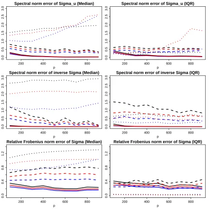
The first setting (Figure 4) represents a heavy-tailed elliptical distribution, where we expect Methods (2), (3), (4) all outperform the POET estimator based on the sample covariance, i.e. Method (1), especially in the presence of extremely heavy tails (solid lines for ν = 3). As expected, all three curves under various measures show error ratios visibly smaller than 1. On the other hand, if data are indeed Gaussian (dotted line for ν =
200 400 600 800
0.0
0.5
1.0
1.5
2.0
2.5
3.0
Spectral norm error of Sigma_u (Median)
p
error r
atio
200 400 600 800
0.0
0.5
1.0
1.5
2.0
2.5
3.0
Spectral norm error of Sigma_u (IQR)
p
error r
atio
200 400 600 800
0.0
0.5
1.0
1.5
2.0
2.5
3.0
Spectral norm error of inverse Sigma (Median)
p
error r
atio
200 400 600 800
0.0
0.5
1.0
1.5
2.0
2.5
3.0
Spectral norm error of inverse Sigma (IQR)
p
error r
atio
200 400 600 800
0.0
0.4
0.8
1.2
Relative Frobenius norm error of Sigma (Median)
p
error r
atio
200 400 600 800
0.0
0.4
0.8
1.2
Relative Frobenius norm error of Sigma (IQR)
p
error r
atio
Figure 4: Error ratios of robust estimates against varying dimension. Blue lines represent errors of Method (2) over Method (1) under different norms; black lines errors of Method (3) over Method (1); red lines errors of Method (4) over Method (1). (ftT, uTt) is generated by multivariate t-distribution with df = 3 (solid), 5 (dashed) and ∞ (dotted). The median errors and their IQR’s (interquartile range) over100 simulations are reported.
leverages the advantage of spatial Kendall’s tau, performs more robustly than Method (3), which solely base its estimation of the eigen-structure on marginal Kendall’s tau.
distribu-200 400 600 800
0.0
0.5
1.0
1.5
2.0
2.5
3.0
Spectral norm error of Sigma_u (Median)
p
error r
atio
200 400 600 800
0.0
0.5
1.0
1.5
2.0
2.5
3.0
Spectral norm error of Sigma_u (IQR)
p
error r
atio
200 400 600 800
0.0
0.5
1.0
1.5
2.0
2.5
3.0
Spectral norm error of inverse Sigma (Median)
p
error r
atio
200 400 600 800
0.0
0.5
1.0
1.5
2.0
2.5
3.0
Spectral norm error of inverse Sigma (IQR)
p
error r
atio
200 400 600 800
0.0
0.4
0.8
1.2
Relative Frobenius norm error of Sigma (Median)
p
error r
atio
200 400 600 800
0.0
0.4
0.8
1.2
Relative Frobenius norm error of Sigma (IQR)
p
error r
atio
Figure 5: Error ratios of robust estimates against varying dimension. Blue lines represent errors of Method (2) over Method (1) under different norms; black lines errors of Method (3) over Method (1); red lines errors of Method (4) over Method (1). (ftT, uTt) is generated by element-wise iid t-distribution with df = 3 (solid), 5 (dashed) and ∞ (dotted). The median errors and their IQR’s (interquartile range) over 100 simulations are reported.
5. Proof organization of main theorems
5.1 Symmetric Case
For shorthand, we write τ = kEk∞, and κ =
√
dkEVkmax. An obvious bound for κ is
κ ≤ √rµ τ (by Cauchy-Schwarz inequality). We will use these notations throughout this subsection.
Recall the spectral decomposition of A in (8). Expressing E in terms of the column vectors ofV and V⊥, which form an orthogonal basis inRn, we write
[V, V⊥]TE[V, V⊥] =:
E11 E12
E21 E22
. (27)
Note that E12 = E21T since E is symmetric. Conceptually, the perturbation results in a rotation of [V, V⊥], and we write a candidate orthogonal basis as follows:
V := (V +V⊥Q)(Ir+QTQ)−1/2, V⊥:= (V⊥−V QT)(Id−r+QQT)−1/2, (28)
where Q ∈ R(d−r)×r is to be determined. It is straightforward to check that [V , V ⊥] is
an orthogonal matrix. We will choose Q in a way such that (V , V⊥)TAe(V , V⊥) is a block
diagonal matrix, i.e.,VT⊥AVe = 0. Substituting (28) and simplifying the equation, we obtain
Q(Λ1+E11)−(Λ2+E22)Q=E21−QE12Q. (29)
The approach of studying perturbation through a quadratic equation is known. See Stewart (1990) for example. Yet, to the best of our knowledge, existing results study perturbation under orthogonal-invariant norms (or unitary-invariant norms in the complex case), which includes a family of matrix operator norms and Frobenius norm, but excludes the matrix max-norm. The advantages of orthogonal-invariant norms are pronounced: such norms of a symmetric matrix only depend on its eigenvalues regardless of eigenvectors; moreover, with suitable normalization they are consistent in the sense kABk ≤ kAk · kBk. See Stewart (1990) for a clear exposition.
The max-norm, however, does not possess these important properties. An imminent issue is that it is not clear how to relateQtoV⊥Q, which will appear in (29) after expanding
Eaccording to (27), and which we want to control. Our approach here is to studyQ:=V⊥Q
directly through a transformed quadratic equation, obtained by left multiplyingV⊥to (29).
Denote H = V⊥E21, Q = V⊥Q, L1 = Λ1 +E11, L2 = V⊥(Λ2+E22)V⊥T. If we can find an
appropriate matrixQ withQ=V⊥Q, and it satisfies the quadratic equation
Q L1−L2Q=H−QHTQ, (30)
then Q also satisfies the quadratic equation (29). This is because multiplying both sides of (30) by V⊥T yields (29), and thus any solution Q to (30) with the form Q= V⊥Q must
result in a solutionQ to (29).
Once we have such Q (or equivalently Q), then (V , V⊥)TAe(V , V⊥) is a block diagonal
eigenvectors, namely span{ev1, . . . ,ver}. We will verify the two spaces are identical in Lemma
7. Before stating that lemma, we first provide bounds onkQkmaxand kV −Vkmax.
Lemma 5 Suppose |λr| −ε > 4rµ(τ + 2rκ). Then, there exists a matrix Q ∈ R(d−r)×r
such that Q = V⊥Q ∈ Rd×r is a solution to the quadratic equation (30), and Q satisfies
kQkmax≤ω/
√
d. Moreover, ifrω <1/2, the matrix V defined in (28) satisfies
kV −Vkmax≤2
√
µ ωr/
√
d . (31)
Here, ω is defined asω = 8(1 +rµ)κ/(|λr| −ε).
The second claim of the lemma (i.e., the bound (31)) is relatively easy to prove once the first claim (i.e., the bound on kQkmax) is proved. To understand this, note that we can rewrite V as V = (V +Q)(Ir+Q
T
Q)−1/2, and kQTQkmax can be controlled by a trivial inequality kQTQkmax ≤dkQk2
max ≤w2. To prove the first claim, we construct a sequence of matrices through recursion that converges to the fixed pointQ, which is a solution to the quadratic equation (30). For all iterates of matrices, we prove a uniform max-norm bound, which leads to a max-bound on kQkmax by continuity. To be specific, we initializeQ
0 = 0, and given Qt, we solve a linear equation:
Q L1−L2Q=H−Q
t
HTQt, (32)
and the solution is defined as Qt+1. Under some conditions, the iterate Qt converges to a limitQ, which is a solution to (30). The next general lemma captures this idea. It follows from Stewart (1990) with minor adaptations.
Lemma 6 Let T be a bounded linear operator on a Banach space B equipped with a norm
k · k. Assume that T has a bounded inverse, and define β =kT−1k−1. Letϕ:B → B be a map that satisfies
kϕ(x)k ≤ηkxk2, and kϕ(x)−ϕ(y)k ≤2ηmax{kxk,kyk}kx−yk (33) for some η ≥ 0. Suppose that B0 is a closed subspace of B such that T−1(B0) ⊆ B0 and
ϕ(B0)⊆ B0. Suppose y∈ B0 that satisfies 4ηkyk< β2. Then, the sequence initialized with
x0 = 0 and iterated through
xk+1=T−1(y+ϕ(xk)), k≥0 (34)
converges to a solution x? to T x = y+ϕ(x). Moreover, we have x? ⊆ B0, and kx?k ≤
2kyk/β.
To apply this lemma to the equation (30), we view B as the space of matrices Rd×r
with the max-norm k · kmax, and B0 as the subspace of matrices of the form V⊥Q where
Q∈R(d−r)×r. The linear operatorT is set to be theT(Q) =Q L1−L2Q, and the mapϕis set to be the quadratic functionϕ(Q) =−QHTQ. Roughly speaking, under the assumption of Lemma 6, the nonlinear effect caused by ϕ is weak compared with the linear operator
T. Therefore, it is crucial to show T is invertible, i.e. to give a good lower bound on
kT−1k−1
issue arises when A is not of exact low rank, which will be discussed at the end of the subsection.
If there is no perturbation (i.e.,E = 0), all the iteratesQtare simply 0, soV is identical toV. If the perturbation is not too large, the next lemma shows that the column vectors of V span the same space as span{ev1, . . . ,evr}.
In other words, with a suitable orthogonal matrixR, the columns ofV Rareev1, . . . ,evr.
Lemma 7 Suppose |λr| −ε >max{3τ,64(1 +rµ)r3/2µ1/2κ}. Then, there exists an
orthog-onal matrix R∈Rr×r such that the column vectors ofV R areve1, . . . ,evr.
Proof of Theorem 2 It is easy to check that under the assumption of Theorem 2, the conditions required in Lemma 5 and Lemma 7 are satisfied. Hence, the two lemmas imply Theorem 2.
To study the perturbation of individual eigenvectors, we assume, in addition to the con-dition on |λr|, that λ1, . . . , λr satisfy a uniform gap, (namely δ > kEk2). This additional assumption is necessary, because otherwise, the perturbation may lead to a change of rel-ative order of eigenvalues, and we may be unable to match eigenvectors from the order of eigenvalues. Suppose R ∈Rr×r is an orthogonal matrix such that V R are eigenvectors of
e
A. Now, under the assumption of Theorem 2, the column vectors ofVe andV Rare identical
up to sign, so we can rewrite the differenceVe −V as
e
V −V =V(R−Ir) + (V −V). (35)
We already provided a bound on kV −Vkmax in Lemma 5. By the triangular inequality, we can derive a bound on kVkmax. If we can prove a bound on kR−Irkmax, it will finally leads to a bound on kVe −Vkmax. In order to do so, we use the Davis-Kahan theorem to
obtain an bound on hvei, vii for all i∈[r]. This will lead to a max-norm bound on R−Ir
(with the price of potentially increasing the bound by a factor of r). The details about the proof of Theorem 3 are in the appendix.
We remark that the conditions on|λr|−in Theorem 2 and Theorem 3 are only useful in
cases where|λr|>kA−Ark∞. Ideally, we would like to have results with assumptions only
involvingλr and λr+1, like in the Davis-Kahan theorem. Unfortunately, unlike orthogonal-invariant norms that only depend on the eigenvalues of a matrix, the max-norm k · kmax is not orthogonal-invariant, and thus it also depends on the eigenvectors of a matrix. For this reason, it is not clear whether we could obtain a lower bound on kT−1k−1
max using only the eigenvaluesλrand λr+1 so that Lemma 6 could be applied. The analysis appears to be difficult if we do not have a bound on kT−1k−1
max, considering that even in the analysis of linear equations, we need invertibility and a well-controlled condition number.
5.2 Asymmetric case
LetAd, Ed bed
1+d2 square matrices defined as
Ad:=
0 A
AT 0
, Ed:=
0 E
ET 0
Also denoteAed:=Ad+Ed. This augmentation of an asymmetric matrix into a symmetric
one is called Hermitian dilation. Here the superscript dmeans the Hermitian dilation. We also use this notation to denote quantities corresponding to Ad and Aed.
An important observation is that
0 A
AT 0
ui
±vi
=±σi
ui
±vi
.
From this identity, we know thatAdhave nonzero eigenvalues ±σi where 1≤i≤rank(A),
and its corresponding eigenvectors are (uTi ,±viT)T. For a given r, we stack these (normal-ized) eigenvectors with indicesi∈[r] into a matrixVd∈R(d1+d2)×2r:
Vd:= √1
2
U U
V −V
.
Through the augmented matrices, we can transfer eigenvector results for symmetric matrices to singular vectors of asymmetric matrices. However, we cannot directly invoke the results proved for symmetric matrices, due to an issue about the coherence of Vd: whend1 andd2 are not comparable, the coherence µ(Vd) can be very large even when µ(V) and µ(U) are bounded. To understand this, consider the case where r= 1, d1d2, and all entries of U areO(1/√d1), and all entries ofV areO(1/
√
d2). Then, the coherencesµ(U) andµ(V) are
O(1), but µ(Vd) =O((d1+d2)/d2)1.
This unpleasant issue about the coherence, nevertheless, can be tackled if we consider a different matrix norm. In order to deal with the different scales of d1 and d2, we define the weighted max-norm for any matrixM with d1+d2 rows as follows:
kMkw :=
√
d1Id1 0
0 √d2Id2
M
max. (36)
In other words, we rescale the topd1 rows ofM by a factor of
√
d1, and rescale the bottom
d2 rows by
√
d2. This weighted norm serves to balance the potential different scales of d1 and d2.
The proofs of theorems in Section 2.2 will be almost the same with those in the symmetric case, with the major difference being the new matrix norm. Because the derivation is slightly repetitive, we will provide concise proofs in the appendix . Similar to the decomposition in (2.1),
Ad=
0 Ar
ATr 0
+
0 A−Ar
AT −ATr 0
=:Adr+ (Ad−Adr),
whereAdr is has rank 2r. Equivalently,
Adr =
r
X
i=1
σi(uTi , viT)T(uTi , vTi )− r
X
i=1
σi(uTi ,−viT)T(uTi,−viT).
simi-lar quantity as |λr|). Recall µ0 = µ(U) ∨µ(V), τ0 = p
d1/d2kEk∞ ∨
p
d2/d1kEk1 and ε0 =
p
d1/d2kA − Ark∞ ∨
p
d2/d1kA − Ark1. In the proof, we will also use
κ0 = max{
√
d1kEVkmax,
√
d2kETUkmax}, which is a quantity similar toκ.
The next key lemma, which is parallel to Lemma 5, provides a bound on the solution
Qd to the quadratic equation
QdLd1−Ld2Qd=Hd−Qd(Hd)TQd. (37)
Lemma 8 Suppose σr − ε0 > 16rµ0(τ0 + rκ0). Then, there exists a matrix Qd ∈
R(d1+d2−2r)×2r such that Qd = V⊥dQd ∈ R(d1+d2)×2r is a solution to the quadratic
equa-tion (37), and Qd satisfieskQdkw ≤ω0. Moreover, if rω0 <1/2, the matrix V
d
defined in (28) satisfies
kVd−Vdkw≤6
√
µ0rω0. (38)
Here, ω0 is defined as ω0 = 8(1 +rµ0)κ0/3(σr−ε0).
In this lemma, the bound (38) bears a similar form to (31): if we consider the max-norm, the firstd1 rows of V
d
−Vdcorrespond to the left singular vectorsu
i’s, and they scale with
1/√d1; and the lastd2 rows correspond to the right singular vectors vi’s, which scale with
1/√d2. Clearly, the weighted max-normk · kw indeed helps to balance the two dimensions.
The rest of the proofs can be found in the appendix.
Acknowledgments
A. Proofs for Section 2.1
Denote the column span of a matrixM by span(M). Suppose two matricesM1, M2∈Rn×m
(m≤n) have orthonormal column vectors. It is known that (Stewart, 1990)
d(M1, M2) :=kM1M1T −M2M2Tk2=ksin Θ(M1, M2)k2. (39) where Θ(M1, M2) are the canonical angles between span(M1) and span(M2). Recall the notations defined in (27), and also recall κ = √dkEVkmax, Λ1 = diag{λ1, . . . , λr}, Λ2 = diag{λr+1, . . . , λn},L1= Λ1+E11,L2 =V⊥(Λ2+E22)V⊥T andH=V⊥E21. The first lemma bounds kHkmax.
Lemma 9 We have the following bound on kHkmax:
kHkmax≤(1 +rµ)κ/√d.
Proof Using the definitionE21 =V⊥TEV in (27), we can write H =V⊥V⊥TEV. Since the
columns ofV and V⊥ form an orthogonal basis in Rd, clearly
V VT +V⊥V⊥T =Id. (40)
By Cauchy-Schwarz inequality and the definition of µ, for anyi, j∈[d],
|(V VT)ij|= r
X
k=1
|VikVjk| ≤ r
X
k=1
Vik21/2
·
r
X
k=1
Vjk21/2
≤ rµ
d .
Using the identity (40) and the above inequality, we derive
kHkmax≤ kEVkmax+kV VTEVkmax
≤(1 +dkV VTkmax)kEVkmax≤(1 +rµ)kEVkmax, which completes the proof.
Lemma 10 If |λr|> κr
√
µ, then L1 is an invertible matrix. Furthermore, inf
kQ0kmax=1
kQ0L1−L2Q0kmax≥ |λr| −3rµ(τ +rκ)−ε , (41)
where Q0 is an d×r matrix.
Proof Let Q0 be anyd×r matrix with kQ0kmax= 1. Note
Q0L1−L2Q0=Q0Λ1+Q0E11−L2Q0.
We will derive upper bounds on Q0E11 and L2Q0, and a lower bound on Q0Λ1. Since
E11=VTEV by definition, we expand Q0E11 and use a trivial inequality to derive
By Cauchy-Schwarz inequality and the definition of µin (3), fori, j∈[d],
|(Q0VT)ij| ≤ r
X
k=1
|(Q0)ikVjk| ≤ r
X
k=1 (Q0)2ik
1/2
r
X
k=1
Vjk21/2 ≤√r·
r
rµ
d ,
Substituting kEVkmax=κ/
√
dinto (42), we obtain an upper bound:
kQ0E11kmax≤κr
√
µ . (43)
To bound L2Q0= (V⊥E22V⊥T + (A−Ar))Q0, we use the identity (40) and write
V⊥E22V⊥TQ0 =V⊥V⊥TEV⊥V⊥TQ0 = (Id−V VT)E(Id−V VT)Q0.
Using two trivial inequalities kEQ0kmax ≤ kEk∞kQ0kmax = kEk∞ and kVTQ0kmax ≤
kVTk∞kQ0kmax≤
√
d, we have
kE(Id−V VT)Q0kmax≤ kEQ0kmax+rkEVkmaxkVTQ0kmax
≤ kEk∞+r
√
dkEVkmax=τ+rκ .
In the proof of Lemma 9, we showedkV VTkmax≤rµ/d. Thus,
kV⊥E22V⊥TQ0kmax≤(1 +dkV VTkmax)· kE(Id−V VT)Q0kmax≤(1 +rµ)(τ +rκ). Moreover,k(A−Ar)Q0kmax≤ kA−Ark∞kQ0kmax=ε. Combining the two bounds,
kL2Q0kmax≤(1 +rµ)(τ+rκ) +ε. (44) It is straightforward to obtain a lower bound on kQ0Λ1kmax: since there is an entry ofQ0, say (Q0)ij, that has an absolute value of 1, we have
kQ0Λ1kmax≥ |(Q0)ijλj| ≥ |λr|. (45)
To show L1 is invertible, we use (42) and (45) to obtain
kQ0L1kmax≥ kQ0Λ1kmax− kQ0E11kmax≥ |λr| −κr
√
µ .
When |λr| −κr
√
µ > 0, L1 must have full rank, because otherwise we can choose an
appropriateQ0 in the null space ofL
T
1 so thatQ0L1 = 0, which is a contradiction. To prove the second claim of the lemma, we combine the lower bound (45) with upper bounds (43) and (44) to derive
kQ0L1−L2Q0kmax≥ kQ0L1kmax− kQ0E11kmax− kL2Q0kmax
≥ |λr| −κr
√
µ−(1 +rµ)(τ+rκ)−ε
≥ |λr| −3rµ(τ +rκ)−ε ,