Robust Principal Component Analysis with Adaptive Selection for
Tuning Parameters
Isao Higuchi [email protected]
Department of Applied Mathematics Hiroshima University
1-4-1, Kagamiyama
Higashi-Hiroshima 739-8527, Japan
Shinto Eguchi [email protected]
Institute of Statistical Mathematics and Graduate University of Advanced Studies 4-6-7, Minami-Azabu, Minato-ku Tokyo 106-8569, Japan
Editor: David Madigan
Abstract
The present paper discusses robustness against outliers in a principal component analysis (PCA). We propose a class of procedures for PCA based on the minimum psi principle, which unifies various approaches, including the classical procedure and recently proposed procedures. The reweighted matrix algorithm for off-line data and the gradient algorithm for on-line data are both investigated with respect to robustness. The reweighted matrix algorithm is shown to satisfy a desirable property with local convergence, and the on-line gradient algorithm is shown to satisfy an asymptotical stability of convergence. Some procedures in the class involve tuning parame-ters, which control sensitivity to outliers. We propose a shape-adaptive selection rule for tuning parameters using K-fold cross validation.
Keywords: K-fold cross validation, on-line algorithm, reweighted matrix algorithm, influence function, data contamination
1. Introduction
In both neural network and statistical studies, PCA is one of the most fundamental tools of dimen-sionality reduction for extracting effective features from high-dimensional vectors of input data. See Croux and Haesbroeck (2000) and De la Torre and Black (2001) for recent discussions. PCA is implemented by projecting input data onto the most informative subspace of lower dimension so that the hidden structure behind the input data may be clarified. The procedure of detecting principal components from input data in an on-line manner is related to the mechanism of a single neuron by the Hebbian adaptation rule, for which the learning theory has been discussed (Amari, 1977; Oja, 1982).
vector or subspace in the PCA. This motivates our study of robust PCA procedures. In what follows, we discuss anε-contamination model for a data distribution Fεdefined by
Fε= (1−ε)N(µ,V) +εH, (1)
where N(µ,V)is a Gaussian distribution with mean vector µ and covariance matrix V , and H is a distribution of possible outliers. In this modeling, it is assumed thatε, or the probability of outliers, is small and that the distribution H is unspecified but qualitatively different from the supposed dis-tribution N(µ,V). Thus, the model (1) lies in a kind ofε-neighborhood surrounding N(µ,V)taking into account all of the possible distributions H. If H has the mean vector µH and the covariance matrix VH, then the data distribution Fεhas the covariance matrix
Vε= (1−ε)V+εVH+ε(1−ε)(µ−µH)(µ−µH)T. (2)
Thus, the classical procedure works properly as long as VH'V and µH'µ, because the procedure
basically searches for the dominant eigenvectors of Vεby learning from input data generated by the assumed distribution Fε. However, even if the probabilityεis quite small, the classical procedure often breaks down when input data have a distribution Fε, such that µHor VHis far from the assumed
µ or V , as observed from (2).
A variety of outlier distributions H have infinite dimensionality, and the simplest candidate is a point-mass distributionδξ(x)degenerated at x=ξ. This choice corresponds to a situation in which the outliers occur deterministically in a singleton ξwith probability ε. The influence function of a procedure in the PCA is defined as the derivative atε=0 of the procedure under Fε in (1) with H=δξ. This concept will be more explicitly explored in a subsequent discussion. See Higuchi and Eguchi (1998) for the case of the PCA, and see Hampel (1974) and Hampel et al. (1986) for the general case.
We discuss a class of principal component analyzers defined using generic functions which con-tain tuning parameters. For example if we adopt a log-sigmoidal function as a generic function, the tuning parameters are the inverse temperature and saturation value parameters, as will be discussed in detail. In general the tuning parameter set makes a delicate trade between loss of information and degree of insensitivity to outliers. The main objective in the present paper is to provide a reasonable selection of tuning parameters of principal component analyzers. The basic idea is to craft a loss function that reflects as appropriate trade off between loss of information and robustness to outliers. We introduce K-fold cross validation for estimating the expected loss based on a given data set. As a result we build a method of data-adaptive selection of tuning parameters. In a simulation study, we examine the performance of the adaptive selection under three types of outlier distributions H displaying deterministic, structural and distributional contaminations based on (2). The three types of outliers are simulated in a numerical experiment, and we test the performance in a few cases of principal component analyzers. We provide an S implementation of the basic robust PCA at
http://home.hiroshima-u.ac.jp/oxbow/RobustPCA/.
2. A Class of Principal Component Vectors
In this section we propose a class of principal component vectors. In general, PCA aims to extract the most informative k-dimensional output vector y from an input vector x of p-dimension. This is achieved by learning the matrixΓwhich connects x to y=ΓT(x−µ) based on input data{x
t;t=
1,2,···}, where µ is a vector of center of the input data and Γ is a p×k orthonormal matrix, or
ΓTΓ=I (the k-identity matrix). In neural networks,Γis interpreted as the matrix of coefficients connecting p neurons to k neurons, where a learning process works by renewingΓaccording to a batch of inputs in an off-line manner or sequential input vectors in an on-line manner (Oja, 1982, 1989 and §8 in Haykin, 1999). By combining these approaches, we propose a certain class of procedures for PCA.
We present a concise review of the classical PCA for detecting the principal k-subspace. Let
z(x,µ,Γ) =1
2{kx−µk 2
− kΓT(x−µ)k2} (3) be half the square of the residual distance of x−µ from the subspace spanned by the columns ofΓ. We note that z(x,µ,Γ) =1
2minβ∈Rkkx−µ−Γβk2. See Hotelling (1933) for the original derivation. The classical PCA is simply given by minimizing
1 n
n
∑
t=1
z(xt,µ,Γ)
with respect to µ andΓ, which reduces to solving k dominant eigenvectors of the sample covariance matrix
S=1
n
n
∑
t=1
(xt−¯µ)(xt−¯µ)T, (4)
where the centralized vector ¯µ is given by∑nt=1xt/n. Thus, we obtain a solutionΓby stacking the k
dominant eigenvectors of S, which we write in the form
Γ=eigen(S).
We propose a variant of this classical procedure for PCA obtained by minimizing an objective function
E
(µ,Γ) = 1n
n
∑
t=1
Ψ(z(xt,µ,Γ)), (5)
whereΨ(z) is assumed to be a monotonic increasing function of z>0. VariousΨyield various procedures for PCA. As typical examples, the identity functionΨ0(z) =z reduces to the classical PCA and
Ψ1(z) =log
1
1+exp{−β(z−η)} (6)
defines Xu and Yuille’s self-organizing rule, where βandηare tuning parameters, referred to as the inverse temperature and saturation value, respectively (Xu and Yuille, 1995). Another possible function is
Ψ2(z) =
1−exp(−βz)
In general,Ψis interpreted as the generic function which gives the total function
E
, and we refer to the minimization ofE
in (5) as the “minimum psi principle generated byΨ”.Based on an argument similar to that of the classical PCA, we observe that the minimizer(˜µ,Γ˜)
of
E
(µ,Γ)satisfies the stationary equations˜µ = n
∑
t=1
pt(˜µ,Γ˜)xt, (8)
˜
Γ = eigen(S(˜µ,Γ˜)), (9)
where
pt(µ,Γ) =
ψ(z(xt,µ,Γ)) ∑n
s=1ψ(z(xs,µ,Γ))
,
S(µ,Γ) = n
∑
t=1
pt(µ,Γ)(xt−µ)(xt−µ)T, (10)
with ψ(z) = (∂/∂z)Ψ(z). Thus, the equilibrium point (˜µ,Γ˜) is expressed by the weighted mean and the covariance matrix, where the weight function pt depends upon ˜µ and ˜Γ, except for the
case ofψ(z) =1, which yields the classical procedure. In effect, (8) is determined only up to the addition of a vector in the subspace associated with ˜Γ. Thus µ∗= ˜µ+γis also a solution of (8) ifγ∈Im(Γ˜)≡ {Γ˜c|c∈Rk}, because µ∗+Im(Γ˜) = ˜µ+Im(Γ˜). However, (9) is independent of the
choice of possible solutions, so we adopt the expression (8) for convenience.
In PCA research, centralization of input data by a vector other than a sample mean has not been considered. In the present paper, we investigate the problem of centralization and explore the usefulness of a method using a vector such as (8). In conventional robust statistics, the estimation of location has been studied extensively. (See, for example, Huber, 1981.) Our estimator ˜µ can be viewed as one of several variants for robust estimation. However, our main objective concerning ˜µ is not the location estimation itself, but rather the data centralization for the extraction of principal components. Thus, ˜µ is naturally linked to ˜Γin the optimization of
E
(µ,Γ).For a batch of data{xt: 1≤t≤n}, we propose a fixed-point algorithm. See Hyvarinen and Oja
(1997) for the related discussion on a fixed-point algorithm for ICA. This algorithm alternates two steps associated with the stationary equations (8) and (9) in the following:
Step 1: Given(µ1,Γ1), calculate
pt(1)=
ψ(z(xt,µ1,Γ1)) ∑n
s=1ψ(z(xs,µ1,Γ1))
.
Step 2: Using the estimated{p(t1)}in step 1, perform the same task as in the classical PCA:
µ2 = n
∑
t=1
p(t1)xt and
Γ2 = eigen(S(1)), (11)
Assuming hereafter that the generic functionΨ(z)is strictly concave in z, we have
E
(µ2,Γ2)−E
(µ1,Γ1)<∑n
t=1ψ(z(xt,µ1,Γ1))
n {
n
∑
t=1
p(t1)z(xt,µ2,Γ2)−
n
∑
t=1
p(t1)z(xt,µ1,Γ1)}
because, by assumption, Ψ(z2)−Ψ(z1)<ψ(z1)(z2−z1)for z1 <z2. In step 2, the procedure is equivalent to minimization of
∑
p(t1)z(xt,µ,Γ)with respect to(µ,Γ). Therefore, we conclude that the RM algorithm generated by{(µj,Γj): j≥1}
is responsible for the strict decrease of the objective function
E
(µ1,Γ1)>···>E
(µj,Γj)>···.This desirable property is mathematically the same as that of the EM algorithm. The possible region of(µ,Γ)that the algorithm works in is
X
×O
p,k, whereX
is the convex hull of data andO
p,k is thespace of p×k orthonormal matrices. We can easily check a condition for the convergence to the solution of the equations such that a set
{(µ,Γ)∈
X
×O
p,k:E
(µ,Γ)≤c}is compact for any fixed c≤
E
(µ1,Γ1). This is referred to as the regularity condition of Wu (1983), found in §3.4.2 of McLachlan and Krishnan (1997), and this condition implies that the sequence{(µj,Γj): j≥1}is convergent to a set of solutions of equations (8) and (9). However, even when
this regularity condition holds, the computational complexity with high dimensional data may be prohibitive since each iteration requires the solution of (11).
2.1 Stability of On-line Gradient Algorithm
We next discuss the on-line gradient algorithm. The gradient vector of the objective function is the sum of
G(µ,Γ)(xt) =ψ(z(xt,µ,Γ))G1(µ,Γ)(xt)
over t=1,2,···, where
G1(µ,Γ)(x) =
x−µ
(x−µ)(x−µ)TΓ−Γ
LT
[yyT]
with y=ΓT(x−µ), where the operator
LT
[·]sets all of the elements above the diagonal of its matrix argument to zero. Hence, the on-line gradient algorithm is given by
µt+1
Γt+1
=
µt
Γt
+rtG(µt,Γt)(xt) (12)
for t =1,2,···with a learning rate rt. If we apply the classical procedure this algorithm reduces
to the Oja algorithm (1982). See §8 in Haykin (1999) for the related algorithmic developments in PCA. The gradient algorithm (12) is different from the Oja algorithm only with respect to the factor ψ(z), which depends on the t-step(µt,Γt) and the t-th example xt through z=z(xt,µt,Γt)
centralization and has no connection toΓ. However, in the case of a non-constant weight function ψ(z), the µ-part is essentially connected not only to µ itself, but also toΓ through the z-variable. For the case of non-constantψ(z), we confine ourselves to the Xu-Yuille rule, which is generated byψ1(z) =β/(1+eβ(z−η)). Xu and Yuille implemented the on-line algorithm in the same fashion as (12) for theΓ-part, but the centralizing mean ¯µ was used for the µ-part. We will make a simple comparison between the two methods for the µ-part in a subsequent discussion.
The on-line gradient algorithm does not satisfy the property of uniform decrease of the objective function possessed by the reweighted algorithm as shown above. We first discuss the asymptotic convergence of (12) for the case of k=1,Γ=γ. See §8.4 in Haykin (1999) for the proof for the classical procedure. The on-line gradient algorithm (12) is a special case of the generic stochastic approximation algorithm
µt+1
γt+1
=
µt
γt
+rth(γt,µt,xt), (13)
where
h(γ,µ,x) =ψ(z(x,µ,γ))
x−µ
(x−µ)(x−µ)Tγ− {γT(x−µ)(x−µ)Tγ}γ
.
Ifψ(z)≡1, then (13) leads to the classical PCA. It is assumed thatψ is a finite function, so the convergence is proved using an argument similar to that used in the case of classical PCA.
Take the expectation of h(γt,µt,xt)over x, and then in the limit we have
¯
h(γ∞,µ∞) = lim
t→∞E[h(γt,µt,xt)]
=
m(γ∞,µ∞)−κ(γ∞,µ∞)µ∞ R(γ∞,µ∞)γ∞− {γT
∞R(γ∞,µ∞)γ∞}γ∞
,
where
κ(γ,µ) =E{ψ(z(x,µ,γ))}, m(γ,µ) =E{ψ(z(x,µ,γ))x}
and
R(γ,µ) =E[ψ(z(x,µ,γ))(x−µ)(x−µ)T].
Thus, our differential equation is
d dt
µt
γt
= h¯(γt)
=
m(γt,µt)−κ(γt,µt)µt R(γt,µ∞)γt− {γT
t R(γt,µ∞)γt}γt
. (14)
In the µ-part, we observe that µt behaves asymptotically as e−κ∞ta+m
∞/κ∞, which implies that m∞/κ∞is the stable-point, whereκ∞=κ(γ∞,µ∞)and m∞=m(γ∞,µ∞). Therefore, we consider only
d
dtγt =R(γt,µ∞)γt− {γtR(γt,µ∞)γt}γt.
We expandγt in terms of the set of eigenvectors{qk(∞): k=1,···,p}of R(γ∞,µ∞)with the domi-nant eigenvector q1(∞)as follows:
Let us decompose ¯h(γ)into ¯h1(γ,γ∞) +h¯2(γ,γ∞), where ¯
h1(γ,γ∞) = R(γ∞,µ∞)γ− {γTR(γ∞,µ∞)γ}γ ¯
h2(γ,γ∞) = {R(γ,µ∞)−R(γ∞,µ∞)}γ (15)
−[γT{R(γ,µ
∞)−R(γ∞,µ∞)}γ]γ.
Then the equilibrium condition ¯h1(γ∞,γ∞) =0 implies thatγ∞reduces to one of k eigenvectors of R(γ∞,µ∞); ¯h2(γ∞,γ∞) =0 holds identically. The differential equation
d dtγt =
¯ h1(γt,γ∞)
has an asymptotically stable point q1(∞)through the same discussion established in §8.4 in Haykin (1999). Hence the differential equation (14) leads to stable convergence to q1(∞).
Secondly, we observe that the case of k principal component vectors also satisfies the stable convergence, noting that our differential equation is
d
dtΓt =R(Γt,µ∞)Γt−
LT
[Γ TtR(Γt,µ∞)Γt]Γt,
where
R(Γ,µ) =E{ψ(z(x,µ,Γ))(x−µ)(x−µ)T}.
In effect, the RM algorithm is applicable to on-line data by solving the eigen problem for batch data with a new observation incorporated in each step. The computational burden is quite heavy relative to the on-line gradient algorithm, but we will pursue more rapid convergence property in a simulation study.
In the statistical literature another type of PCA methods has been proposed by minimizing
1 n
n
∑
t=1
Ψ(d(xt,µ,V))
with respect to(µ,V), where d is Mahalanobis squared distance, that is,
d(xt,µ,V) =
1
2(xt−µ) TV−1(x
t−µ).
See Campbell(1980), Devlin et al. (1981), Caussinus and Ruiz (1990), and Croux and Haesbroeck (2000). The use of the nonlinear generic functionΨis the same, but the essential difference is that our method aims at estimating the principal component vectors rather than estimating the scatter matrix V . One advantage of our method is that it does not need all the information of V . In fact only the first k dominant eigenvalues and the corresponding eigenvectors are needed in the algorithm, which is easily implemented by the singular-value decomposition algorithm even if the data set is of high dimension.
3. Robustness of the Proposed Principal Component Vectors
complement. As a result, the PCA fails to capture an important feature of the bulk of the data, which will be observed from a simple simulation study in Section 5. In the statistical literature, the robustification of the classical likelihood-based procedures has been discussed and well established: see Huber (1981) for some notions on robustness. Such contamination is typically expressed by the ε-contamination model,
(1−ε)N(µ,V)(x) +εδξ(x),
with the point-mass distributionδξas discussed in the Introduction. In the expression, εis unde-tectably small; nevertheless, the likelihood procedure based on the density function of N(µ,V)may sometimes break down for an extreme vectorξ. We next explore which first principal component vector or principal subspace is robust against outliers in our class. First, we consider the case of the first principal component vector, or k=1. In Higuchi and Eguchi (1998), the influence function of the Xu and Yuille rule defined byΨ1in (6) is given by
IFΨ1(ξ) =−ψ1(z(ξ,µ,γ1))˜γT1(ξ−µ)
p
∑
j=2 ˆ
λj˜γTj(ξ−µ)
˜
λj(λˆj−ˆλ1) ˜ γj,
where(λˆj,ˆγj)is the pair of the j-th dominant eigenvalue and its associated eigenvector of S defined
at (4) and(λ˜j,˜γj)is that of S(µ,Γ)defined at (10), and
ψ1(z) =∂Ψ1
(z)
∂z =
β
1+exp{β(z−η)}. (16)
The influence function assesses the effect on the principal component subspace of the contami-nation of the data{xt|1≤t≤n}by the outlierξ.
Secondly, we discuss a general case of k principal component vectors Γ= (γ1, . . . ,γk). We consider the matrix
P=ΓΓT.
The matrix P is the projection operator onto the subspace spanned by the eigenvectorsγI, see Tanaka (1988). Our estimator ˜P=Γ˜Γ˜Thas the influence function
IFΨ1(ξ; ˜P) =−ψ1(z(ξ,˜µ,Γ˜))
∑
ˆλjγ˜IT(ξ−˜µ)(ξ−˜µ)Tγ˜j
˜
λj(λˆj−ˆλI)
(γ˜Iγ˜Tj+γ˜jγ˜TI), (17)
where the summation is taken over{(I,j): I =1,···,k,j=1,···,p,I6= j}, and we will also use this summation convention in a subsequent discussion.
The formula is valid for the minimum psi principle for a generalΨ, see Kamiya and Eguchi (2001) for a detailed discussion, as well as a discussion of relative efficiency under a Gaussian distribution. The influence function, as a function ofξ, assesses the smoothness of the principal component subspace around the supposed distribution N(µ,V). The boundedness of the influence function inξqualitatively guarantees robustness for the target principal component subspace.
In PCA, µ needs to be estimated in order to centralize the data before extracting the principal component subspace. This is usually estimated as∑xt/n, which can be expressed in the form of a
functionalR
xdF(x)with F=Fn(empirical distribution). This usual estimation is Fisher consistent
sinceR
our PCA procedure automatically leads to a robust centralization of data. We typically observe an unbounded case for the usual principal component subspace, and a bounded case for Xu and Yuille’s principal component subspace.
The boundedness of IFΨconditional on
kΓ˜T(ξ−˜µ)k2≤d2 (18) with a positive constant d guarantees robustness against any outliersξ satisfying (18) in the con-tamination model, cf. Higuchi and Eguchi (1998) for the justification for this robustness. Using the formula (17) with generalΨ, we find a sufficient condition for the robustness
sup
z>0
√
zψ(z)<∞ (19)
withψ(z) =∂Ψ(z)/∂z. The proof is given as follows. First, we obtain
kIFΨ(ξ; ˜P)k ≤ ψ(z(ξ,˜µ,Γ˜))
∑
ˆλjγ˜IT(ξ−˜µ)(ξ−˜µ)Tγ˜j
˜
λj(ˆλj−λˆI)
kγ˜Iγ˜Tj+γ˜jγ˜TIk
≤ d
∑
ˆ
λjk˜γIγ˜Tj +γ˜j˜γTIk
˜
λj(λˆj−ˆλI)
|(ξ−˜µ)Tγ˜
j|ψ(z(ξ,˜µ,Γ˜))
from the assumption of (18). Since
z(ξ,˜µ,Γ˜) =1 2
p
∑
j=k+1
{˜γTj(ξ−˜µ)}2≥1 2{˜γ
T
j(ξ−˜µ)}2
for any j, k+1≤ j≤p by the definition of z at (3), we obtain
kIFΨ(ξ; ˜P)k ≤
∑
ˆλjkγ˜Iγ˜Tj+γ˜jγ˜TIk
˜
λj(ˆλj−λˆI)
d√2
q
z(ξ,˜µ,Γ˜)ψ(z(ξ,˜µ,Γ˜)) +d2ψ(z(ξ,˜µ,Γ˜))
.
Finally, we conclude that
kIFΨ(ξ; ˜P)k ≤C
d√2 sup
z>0
√
zψ(z) +d2sup
z>0 ψ(z)
for any outlierξin Rpsatisfying (18), where
C=
∑
ˆλjkγ˜Iγ˜Tj+γ˜jγ˜TIk
˜
λj(ˆλj−λˆI) .
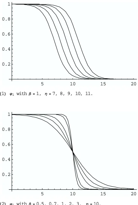
5 10 15 20 0.2
0.4 0.6 0.8 1
H1L ϕ1 withβ =1, η =7, 8, 9, 10, 11.
5 10 15 20
0.2 0.4 0.6 0.8 1
H2L ϕ1 withβ =0.5, 0.7, 1, 2, 3, η =10.
5 10 15 20
0.2 0.4 0.6 0.8 1
H3L ϕ2 withβ =0.1, 0.2, 0.5.
Fig. 1. Graphs of for several tuning parameters.ϕ
4. Adaptive Selection for Tuning Parameters
Letα be a parameter in the generic function Ψwhich defines our objective function (5). In this section, we focus on the role of the tuning parameterα. The performance of PCA by the proposed method generated byΨαdepends on the value of the tuning parameterα. As shown in (6) and (7), the generic functionΨ1involves tuning parametersβandη, andΨ2involvesβ.
Thus, generic functions control the sensitivity to outliers by these tuning parameters. See Fig-ure 1 for the graphs of the derivativesψ1andψ2ofΨ1andΨ2for several tuning parameters.
The generic functionΨ1whereη→∞orβ→0 yields the classical PCA. If we exactly assume Gaussian distribution, orε=0 in (1), then the classical PCA orψ(z)≡1, is recommended as the standard method. See Kamiya and Eguchi (2001) for a detailed discussion. This suggests that under the situation in whichε6=0, there exists an optimal selection for tuning parameters giving a generic function other thanψ(z)≡1.
We propose herein a method of determining tuning parameters as in (6) and (7), based on K-fold cross-validation. See Subsection 7.10 in Hastie et al. (2001) for the detailed discussion. Throughout the section, we focus on batch data.
Let F(x)be a data distribution which is assumed to generate input data x. Then, we adopt a generalization error function for assessing the performance of a given ˆµ and ˆΓusing
L(θˆ,F) =
Z
···
Z
Ψ0(z(x,ˆµ,Γˆ))dF(x) where
Ψ0(z) =log
1
1+exp{−β0(z·η0)}
withα0= (β0,η0) = (50,10). This choice of the error function is intended to achieve mild robust-ness to outliers. This is because we cannot obtain a sensible result if the error function itself is sensitive to outliers. The empirical error function is
Lemp(θˆ) = 1 n
n
∑
t=1
Ψ0(z(xt,ˆµ,Γˆ))
for given data {x1, . . . ,xn} and would be unchanged by data contamination if (ˆµ,Γˆ) is a robust
estimator. The choice ofβ0is universal, but that ofη0should be adaptive. For example, the median ofkxI−¯µkwith the usual centralizing vector ¯µ as a default value. Given a class of estimatorsˆθα
by the generic functionΨαwith the tuning parameter α, for exampleα= (β,η) in (6) or (7), we attempt to estimate the expected loss function, or the risk function associated with an estimator ˆθα, which is essentially
R(θˆα,F) =EF{L(θˆα,F)},
where EF denotes the mathematical expectation when input data x1,···,xnfollow from the
under-lying distribution F.
Here we provide a method of selectingα∗which generates ˆθα∗ with good performance. We use
K-fold validation to get a estimator of the generalization error L(θˆα,F). Here, we divide the data set D={x1, . . . ,xn}into K subsets{Dk={x(1k), . . . ,x
(k)
nk }: k=1,···,K}and so D= SK
k=1Dk. Define
CV(α) = 1
K
K
∑
k=1 L(empk) (θˆ
(−k)
where ˆθ(α−k)is the estimator based on the data setS
k06=kDk0 and
Lemp(k) (θ) = 1 nk
nk
∑
I=1
L(x(Ik),θ).
In this way, the estimator ˆθαand Dk are statistically independent, which implies elimination of the
bias in the empirical error Lemp(θˆα). In this formulation, we now define the optimalα∗by α∗=argmin
α CV(α).
We will explore the performance of this selection method for synthetic data situations.
5. Simulation Study
We explore the robustness of our class of principal component subspaces in numerical experiments, focusing on the classical rule (ψ(z) =1), the Xu-Yuille rule and the Gaussian kernel rule defined in (7). For our simulation study, we consider the following three types of outlier distributions H in the ε-contamination model defined by (1):
(i) Deterministic contamination: a sum of point-mass distributions at x=ξj for j=1,···,M.
(ii) Structural contamination: the same Gaussian distribution N(µ1,V1), but with the structure in µ1and V1being quite different from with that in µ and V , that is to say,kµ1−µkor tr(V1−V)2 is substantially large.
(iii) Distributional contamination: the same structure as in (µ,V) but the distribution is totally different from the Gaussian distribution N(µ,V).
First, we investigate the case in which ε is undetectably small, for example we take ε=0.03. We have performed a numerical study for the behavior of our procedure for seven-dimensional data in the following setting: µ= (0,···,0)T,V =diag(5,2,3,1,0.5,0.5,0.5). As for (i), ξ
1=
(0,0,0,0,0,0,b),ξ2= (0,0,0,0,0,b,0)with a probability 0.5 for each. In (ii) the distribution H is a Gaussian distribution with
µ1= (1,···,1)T,V
1=diag(0.5,2,3,1,0.5,0.5,0.5).
In (iii) the outlier, ξ has a distribution H of Cauchy-type of which the location-scatter structure is the same as(µ,V), that is, all the components of V−12(ξ−µ)are independently and identically
distributed according to a standard Cauchy distribution with density function 1/(π(1+x2)). We observe in a series of simulations in the above setting that the classical procedure(ψ(z) =1)
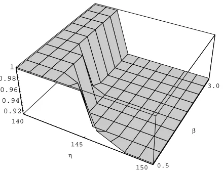
0.92 0.94 0.96 0.98 1
150 145
140
0.5
3.0
β
η
Figure 2: The plot of inner product of the PC vectors with/without outliers againstβandη.
occurrence than for setting (ii). In almost all of the cases of setting (iii), the PCA breaks down. Thus, we observe that the distributional contamination is more severe than the structural contamination for the classical PCA.
We confine ourselves to a typical case of input vectors from the structural contamination. We obtained 270 input vectors of 200-dimension from N(µ,V), where
µ= (0,···,0)T, V =diag(10,9,8,7,6,5,4,3,2,1,0.5,···,0.5), and 30 outliers from N(µ1,V1), where
µ1= (1,···,1)T, V1=diag(1,9,8,7,6,5,4,3,2,1,1,1,···,1),
and observed that the inner product of the first principal component vectors based on the data of 270 vectors and on the data added to 30 outliers is 0.678 when using the classical PCA. On the other hand the inner product is 0.999 using procedure defined by (16) withβ=0.5 andη=130. The RM algorithm is started with the initial vectorγ= (1/√200,···,1/√200)T and µ= (0,···,0), which assigns less weight to the 30 outliers after 10 iterations.
In this procedure, we heuristically choose the tuning parametersβandη. We observe in Figure 2 that the performance is not so sensitive to the choice ofβifη<145. In the subsequent simulation, we will investigate the data-adaptive selection for tuning parameters using the 10-fold CV method in Section 4.
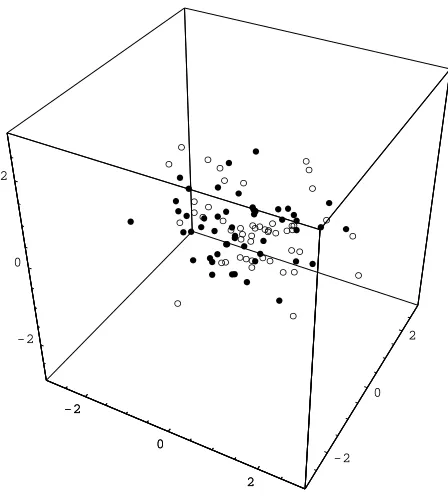
-2 0 2 -2 0 2 -2 0 2 o o o o o o o o o o o o o o o o o o o o o o o o o oo o o o o o o o o o o o o o o o o o o
o o o o o
-2
0
2
Figure 3: The plot of 50 observations and 50 outliers in the minor subspace.
principal component vectors with and without 50 outliers by the classical procedure. Alternatively our procedure gives 0.833, so we see that the procedure can detect a more sensible direction vector than the classical procedure. The proposed procedure detects the heterogeneity of structure, as indicated in Figure 4. If we have more information on the contamination or outlying structure, then we can build a shaper model for the outlier distribution. For example, we might suggest a two component Gaussian mixture model and estimate the structure in a more complete situation via the EM algorithm. However, to expect exact information on the outliers is often unrealistic in the present situation.
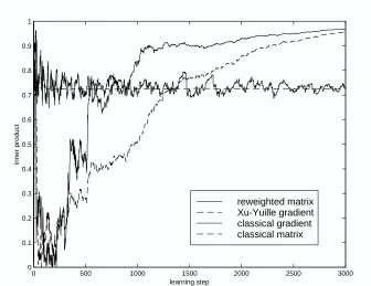
We apply the RM algorithm to on-line input vectors for comparison with the gradient learning algorithm. For the simulation study, we assume a specific form of model (ii) with ε=0.1 and Gaussian density with µ=0, µ1= (30,0,0,0,30)T, V=diag(9,7,5,3,1), and V1=diag(1,1,3,3,5). Thus, the true principal component vector of V is(1,0,0,0,0)in the simulation design. We observe that the RM algorithm is stable and attains rapid convergence from these on-line input vectors. However, the computational burden is much heavier than the on-line gradient algorithm, as shown in Figure 5.
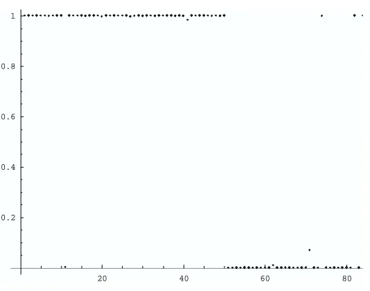
20 40 60 80 0.2
0.4 0.6 0.8 1
Fig. 4. The plot of the weight function of psi over 50 data with 50 outliers.
Figure 4: The plot of the weight function ofψover 50 data with 50 outliers.
We propose a robust procedure for centralization of the data in (12). In the neural networks liter-ature, such a variant for centralizing data has been ignored until now. Using the usual centralization is correct if all of the data are generated from Gaussian distribution. This is because the mean vector and covariance matrix are orthonormal as parameters, so that any influence on the principal vectors is independent of that on the mean vector. However, if the data in the mean vector are structured, this sometimes has a significant impact on the PCA. Here we consider a simple simulation study for investigating the difference between two procedures defined by adopting the weighted sample mean vector ˆµ in the RM algorithm and the sample mean vector ¯µ in classical PCA as the centralizer. We generate 180 observations from a Gaussian density N(0,V)with V =diag(9,7,5,3,1)and 20 outliers from N((0,0,20,0,0)T,V). Figure 7 shows the two-dimensional score plot produced by the classical PCA based on only the 180 observations without any outliers, where the horizontal axis is taken as taken exactly as the first principal component vector. We observe that the first principal component vector by ˆµ-centralization yields a proper direction.
6. Discussion
0 500 1000 1500 2000 2500 3000 0
0.1 0.2 0.3 0.4 0.5 0.6 0.7 0.8 0.9 1
learning step
inner product
reweighted matrix Xu-Yuille gradient classical gradient classical matrix
Fig. 5. The inner products of the true vector (1,0,0,0) and the PC vectors by RM, Xu-Yuille gradient, the classical gradient and classical matrix algorithms.
Figure 5: The inner products of the true vector(1,0,0,0) and the PC vectors by RM, Xu-Yuille gradient, the classical gradient and classical matrix algorithms.
Our major point is the adaptive selection of a set of tuning parameters which control the degree of robustification. In empirical studies, we observe that the robustness performance is sensitive to the selection of tuning parameters. K-fold cross validation properly gives the adaptive selection for tuning parameters in accordance with data. However the selection method is done only for batch data but it cannot be applied to on-line data, which we must post as a future research. The RM algorithm needs the evaluation of eigenvalues and eigenvectors of the full matrix. In this respect it requires heavy computational burdens, whereas the convergence is stable and rapid relative to the gradient algorithm. The RM algorithm must be improved when the dimension of the input vector is considerably high. There is room for improvement in solving the k-dominant eigenvectors from a computational point of view.
5 10 15 20 25 -126
-124 -122
Fig. 6. The plot of 10-fold CV for the Xu-Yuille rule for =1 fixed.
η
β
Figure 6: The plot of 10-fold CV for the Xu-Yuille rule forβ=1 fixed.
References
Amari, S. -I. Neural theory of association and concept formation. Biological Cybernetics, 26, 175– 185, 1977.
Campbell, N. A. Robust procedures in multivariate analysis 1: Robust covariance estimation. Ap-plied Statistics 29, 231-237, 1980.
Caussinus, H. and Ruiz, A. Interesting projections of multidimensional data by means of general-ized principal component analysis. COMPSTAT 90, 121–126, 1990.
Croux, C. and Haesbroeck, G. Principal component analysis based on robust estimators of the co-variance or correlation matrix: Influence functions and efficiencies. Biometrika, 87, 603-618, 2000.
De la Torre, F. and Black, M. Robust principal component analysis for computer vision. Interna-tional Conference on Computer Vision, 2001.
Hampel, F. R. The influence curve and its role in robust estimation. Journal of the American Statis-tical Association, 69, 383–393, 1974.
Hampel, F. R., Ronchetti, E. M., Rousseeuw, P. J. and Stahel, W. A. Robust Statistics: the Approach Based on Influence Functions. Wiley, 1986.
Hastie, T. J., Tibshirani, R. J. and Friedman, J. H. The Elements of Statistical Learning: Data Mining, Inference, and Prediction. Springer-Verlag, 2001.
-10 -5 0 5 10 15 -10
-5 0 5 10 15
1st PC
2nd PC
Data Outliers
1
v
2
Fig.7. The effect of centlization ways.
γ ( µ ) γ ( µ )
^
^ ^ _
Figure 7: The effect of centralization ways.
Higuchi, I. and Eguchi, S. The influence function of principal component analysis by self-organizing rule. Neural Computation, 10, 1435–1444, 1998.
Hotelling, H. Analysis of a complex of statistical variables into principal components. Journal of Educational Psychology, 24, 417–441, 1933.
Huber, P. J. Robust Statistics. Wiley, 1981.
Hyvarinen, A. and Oja, E. A fast fixed-point algorithm for independent component analysis. Neural Computation, 9, 1483–1492, 1997
Kamiya, H. and Eguchi, S. A class of robust principal component vectors. Journal of Multivariate Analysis, 76, 239–269, 2001.
McLachlan, G. J. and Krishnan, T. The EM Algorithm and Extensions. Wiley, 1997.
Oja, E. A simplified neuron model as a principal component analyzer. Journal of Mathematical Biology, 15, 267–273, 1982.
Tanaka, Y. Sensitivity analysis in principal component analysis: influence on the subspace spanned by principal components. Communications in Statistics -Theory and Methods, 17, 3157–3175, 1988.
Wu, C. F. J. On the convergence properties of the EM algorithm. Annals of Statistics, 11, 95–103, 1983.