Variational Message Passing

(1)

Variational Message Passing

Christopher M. Bishop [email protected]

Microsoft Research Cambridge Roger Needham Building 7 J. J. Thomson Avenue Cambridge CB3 0FB, U.K.

Editor: Tommi Jaakkola

Abstract

Bayesian inference is now widely established as one of the principal foundations for machine learn-ing. In practice, exact inference is rarely possible, and so a variety of approximation techniques have been developed, one of the most widely used being a deterministic framework called varia-tional inference. In this paper we introduce Variavaria-tional Message Passing (VMP), a general purpose algorithm for applying variational inference to Bayesian Networks. Like belief propagation, VMP proceeds by sending messages between nodes in the network and updating posterior beliefs us-ing local operations at each node. Each such update increases a lower bound on the log evidence (unless already at a local maximum). In contrast to belief propagation, VMP can be applied to a very general class of conjugate-exponential models because it uses a factorised variational approx-imation. Furthermore, by introducing additional variational parameters, VMP can be applied to models containing non-conjugate distributions. The VMP framework also allows the lower bound to be evaluated, and this can be used both for model comparison and for detection of convergence. Variational message passing has been implemented in the form of a general purpose inference en-gine called VIBES (‘Variational Inference for BayEsian networkS’) which allows models to be specified graphically and then solved variationally without recourse to coding.

Keywords: Bayesian networks, variational inference, message passing

1. Introduction

(2)

However, Monte Carlo methods are computationally very intensive, and also suffer from dif-ficulties in diagnosing convergence, while belief propagation is only guaranteed to converge for tree-structured graphs. Expectation propagation is limited to certain classes of model for which the required expectations can be evaluated, is also not guaranteed to converge in general, and is prone to finding poor solutions in the case of multi-modal distributions. For these reasons the framework of variational inference has received much attention.

In this paper, the variational message passing algorithm is developed, which optimises a varia-tional bound using a set of local computations for each node, together with a mechanism for pass-ing messages between the nodes. VMP allows variational inference to be applied automatically to a large class of Bayesian networks, without the need to derive application-specific update equa-tions. In VMP, the messages are exponential family distributions, summarised either by their natural parameter vector (for child-to-parent messages) or by a vector of moments (for parent-to-child mes-sages). These messages are defined so that the optimal variational distribution for a node can be found by summing the messages from its children together with a function of the messages from its parents, where this function depends on the conditional distribution for the node.

The VMP framework applies to models described by directed acyclic graphs in which the con-ditional distributions at each node are members of the exponential family, which therefore includes discrete, Gaussian, Poisson, gamma, and many other common distributions as special cases. For example, VMP can handle a general DAG of discrete nodes, or of lineGaussian nodes, or an ar-bitrary combination of the two provided there are no links going from continuous to discrete nodes. This last restriction can be lifted by introducing further variational bounds, as we shall discuss. Fur-thermore, the marginal distribution of observed data represented by the graph is not restricted to be from the exponential family, but can come from a very broad class of distributions built up from exponential family building blocks. The framework therefore includes many well known machine learning algorithms such as hidden Markov models, probabilistic PCA, factor analysis and Kalman filters, as well as mixtures and hierarchical mixtures of these.

Note that, since we work in a fully Bayesian framework, latent variables and parameters appear on an equal footing (they are all unobserved stochastic variables which are marginalised out to make predictions). If desired, however, point estimates for parameters can be made simply by maximising the same bound as used for variational inference.

As an illustration of the power of the message passing viewpoint, we use VMP within a software tool called VIBES (Variational Inference in BayEsian networkS) which allows a model to be speci-fied by drawing its graph using a graphical interface, and which then performs variational inference automatically on this graph.

The paper is organised as follows. Section 2 gives a brief review of variational inference meth-ods. Section 3 contains the derivation of the variational message passing algorithm, along with an example of its use. In Section 4 the class of models which can be handled by the algorithm is de-fined, while Section 5 describes the VIBES software. Some extensions to the algorithm are given in Section 6, and Section 7 concludes with an overall discussion and suggestions for future research directions.

2. Variational Inference

(3)

by X= (V,H)where V are the visible (observed) variables and H are the hidden (latent) variables. We assume that the model has the form of a Bayesian network and so the joint distribution P(X)

can be expressed in terms of the conditional distributions at each node i,

P(X) =

∏

i

P(Xi|pai) (1)

where pai denotes the set of variables corresponding to the parents of node i and Xi denotes the

variable or group of variables associated with node i.

Ideally, we would like to perform exact inference within this model to find posterior marginal distributions over individual latent variables. Unfortunately, exact inference algorithms, such as the junction tree algorithm (Cowell et al., 1999), are typically only applied to discrete or linear-Gaussian models and are computationally intractable for all but the simplest models. Instead, we must turn to approximate inference methods. Here, we consider the deterministic approximation method of variational inference.

The goal in variational inference is to find a tractable variational distribution Q(H)that closely approximates the true posterior distribution P(H|V). To do this we note the following decomposi-tion of the log marginal probability of the observed data, which holds for any choice of distribudecomposi-tion:

Q(H)

ln P(V) =

L

(Q) +KL(Q||P). (2)

Here

L

(Q) =

∑

H

Q(H)lnP(H,V)

Q(H) (3)

KL(Q||P) = −

∑

H

Q(H)lnP(H|V)

Q(H)

and the sums are replaced by integrals in the case of continuous variables. Here KL(Q||P)is the Kullback-Leibler divergence between the true posterior P(H|V)and the variational approximation

Q(H). Since this satisfies KL(Q||P)>0 it follows from (2) that the quantity

L

(Q)forms a lower bound on ln P(V).

We now choose some family of distributions to represent Q(H)and then seek a member of that family that maximises the lower bound

L

(Q)and hence minimises the Kullback-Leibler divergence KL(Q||P). If we allow Q(H) to have complete flexibility then we see that the maximum of the lower bound occurs when the Kullback-Leibler divergence is zero. In this case, the variational posterior distribution equals the true posterior and

L

(Q) =ln P(V). However, working with the true posterior distribution is computationally intractable (otherwise we wouldn’t be resorting to variational methods). We must therefore consider a more restricted family of Q distributions which has the property that the lower bound (3) can be evaluated and optimised efficiently and yet which is still sufficiently flexible as to give a good approximation to the true posterior distribution.

(4)

2.1 Factorised Variational Distributions

We wish to choose a variational distribution Q(H)with a simpler structure than that of the model, so as to make calculation of the lower bound

L

(Q)tractable. One way to simplify the dependency structure is by choosing a variational distribution where disjoint groups of variables are independent. This is equivalent to choosing Q to have a factorised form

Q(H) =

∏

i

Qi(Hi), (4)

where {Hi}are the disjoint groups of variables. This approximation has been successfully used

in many applications of variational methods (Attias, 2000; Ghahramani and Beal, 2001; Bishop, 1999). Substituting (4) into (3) gives

L

(Q) =

∑

H

∏

i

Qi(Hi)ln P(H,V)−

∑

i

∑

Hi

Qi(Hi)ln Qi(Hi).

We now separate out all terms in one factor Qj,

L

(Q) =

∑

Hj

Qj(Hj)hln P(H,V)i∼Qj(Hj)+H(Qj) +

∑

i6=j H(Qi)

= −KL(Qj||Q?j) +terms not in Qj (5)

whereHdenotes entropy and we have introduced a new distribution Q?_j, defined by

ln Q?_j(Hj) =hln P(H,V)i∼Q(Hj)+const. (6)

andh·i∼Q(Hj)denotes an expectation with respect to all factors except Qj(Hj). The bound is

max-imised with respect to Qj when the KL divergence in (5) is zero, which occurs when Qj =Q?j.

Therefore, we can maximise the bound by setting Qjequal to Q?j. Taking exponentials of both sides

we obtain

Q?_j(Hj) = 1

Zexphln P(H,V)i∼Q(Hj), (7)

where Z is the normalisation factor needed to make Q?_j a valid probability distribution. Note that the equations for all of the factors are coupled since the solution for each Qj(Hj)depends on

expec-tations with respect to the other factors Qi6=j. The variational optimisation proceeds by initialising

each of the Qj(Hj)and then cycling through each factor in turn replacing the current distribution

with a revised estimate given by (7).

3. Variational Message Passing

In this section, the variational message passing algorithm will be derived and shown to optimise a factorised variational distribution using a message passing procedure on a graphical model. For the initial derivation, it will be assumed that the variational distribution is factorised with respect to each hidden variable Hi and so can be written

Q(H) =

∏

i

Qi(Hi).

From (6), the optimised form of the jth factor is given by

(5)

. . .

ch

j

cp

(_kj)

≡

pa

k

\

H

j

pa

j

H

j

X

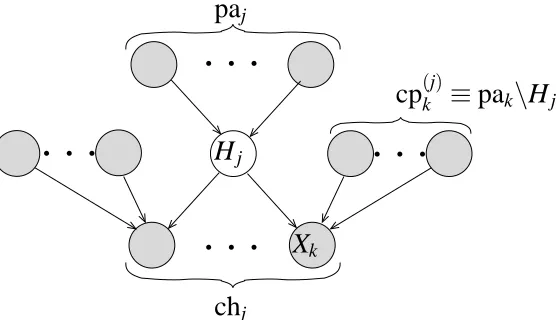
k

Figure 1: A key observation is that the variational update equation for a node Hj depends only on

expectations over variables in the Markov blanket of that node (shown shaded), defined as the set of parents, children and co-parents of that node.

We now substitute in the form of the joint probability distribution of a Bayesian network, as given in (1),

ln Q?_j(Hj) =

∑

iln P(Xi|pai)

∼Q(Hj)+const.

Any terms in the sum over i that do not depend on Hj will be constant under the expectation and

can be subsumed into the constant term. This leaves only the conditional P(Hj|paj)together with

the conditionals for all the children of Hj, as these have Hj in their parent set,

ln Q?_j(Hj) =hln P(Hj|paj)i∼Q(Hj)+

∑

_k_∈ch_jhln P(Xk|pak)i∼Q(Hj)+const. (8)

where chj are the children of node j in the graph. Thus, the expectations required to evaluate Q?j

involve only those variables lying in the Markov blanket of Hj, consisting of its parents, children

and co-parents1cp(j)_k . This is illustrated in the form of a directed graphical model in Figure 1. Note that we use the notation Xk to denote both a random variable and the corresponding node in the

graph. The optimisation of Qj can therefore be expressed as a local computation at the node Hj.

This computation involves the sum of a term involving the parent nodes, along with one term from each of the child nodes. These terms can be thought of as ‘messages’ from the corresponding nodes. Hence, we can decompose the overall optimisation into a set of local computations that depend only on messages from neighbouring (i.e. parent and child) nodes in the graph.

3.1 Conjugate-Exponential Models

The exact form of the messages in (8) will depend on the functional form of the conditional distri-butions in the model. It has been noted (Attias, 2000; Ghahramani and Beal, 2001) that important simplifications to the variational update equations occur when the distributions of variables,

(6)

tioned on their parents, are drawn from the exponential family and are conjugate2 with respect to the distributions over these parent variables. A model where both of these constraints hold is known as a conjugate-exponential model.

A conditional distribution is in the exponential family if it can be written in the form

P(X|Y) =exp[φ(Y)Tu(X) +f(X) +g(Y)] (9) whereφ(Y)is called the natural parameter vector and u(X)is called the natural statistic vector. The term g(Y)acts as a normalisation function that ensures the distribution integrates to unity for any given setting of the parameters Y. The exponential family contains many common distributions, including the Gaussian, gamma, Dirichlet, Poisson and discrete distributions. The advantages of exponential family distributions are that expectations of their logarithms are tractable to compute and their state can be summarised completely by the natural parameter vector. The use of conjugate distributions means that the posterior for each factor has the same form as the prior and so learning changes only the values of the parameters, rather than the functional form of the distribution.

If we know the natural parameter vector φ(Y)for an exponential family distribution, then we can find the expectation of the natural statistic vector with respect to the distribution. Rewriting (9) and definingg as a reparameterisation of g in terms ofe φgives,

P(X|φ) =exp[φTu(X) +f(X) +eg(φ)].

We integrate with respect to X,

Z

X

exp[φT_u₍_X_{) +}_f₍_X_{) +}

e

g(φ)]dX=

Z

X

P(X|φ)dX = 1

and then differentiate with respect toφ

Z

X d dφexp[φ

T_u₍_X_{) +} _f₍_X_{) +}

e

g(φ)]dX = d

dφ(1) = 0

Z

X

P(X|φ)

u(X) + deg(φ) dφ

dX = 0.

And so the expectation of the natural statistic vector is given by

hu(X)i_P(_X|_φ₎ = −dge(φ)

dφ . (10)

We will see later that the factors of our Q distribution will also be in the exponential family and will have the same natural statistic vector as the corresponding factor of P. Hence, the expectation of u under the Q distribution can also be found using (10).

3.2 Optimisation of Q in Conjugate-Exponential Models

We will now demonstrate how the optimisation of the variational distribution can be carried out, given that the model is conjugate-exponential. We consider the general case of optimising a factor

(7)

. . .

pa

_Y

cp

_Y

ch

Y

X

Y

Figure 2: Part of a graphical model showing a node Y , the parents and children of Y , and the co-parents of Y with respect to a child node X .

Q(Y)corresponding to a node Y , whose children include X , as illustrated in Figure 2. From (9), the log conditional probability of the variable Y given its parents can be written

ln P(Y|pa_Y) =φ_Y(pa_Y)T_uY₍_Y_{) +}_f

Y(Y) +gY(paY). (11)

The subscript Y on each of the functions φ_Y,uY,fY,gY is required as these functions differ for

different members of the exponential family and so need to be defined separately for each node. Consider a node X∈chYwhich is a child of Y . The conditional probability of X given its parents

will also be in the exponential family and so can be written in the form

ln P(X|Y,cp_Y) =φ_X(Y,cp_Y)TuX(X) +fX(X) +gX(Y,cpY) (12)

where cp_Y are the co-parents of Y with respect to X , in other words, the set of parents of X excluding

Y itself. The quantity P(Y|pa_Y)in(11) can be thought of as a prior over Y , and P(X|Y,cp_Y)as a (contribution to) the likelihood of Y .

E

x

a

m

p

le If X is Gaussian distributed with mean Y and precision_{contains only}_{β, and the log conditional for X is} β, it follows that the co-parent set cpY

ln P(X|Y,β) =

_βY

−β/2 T

X X2

+1

2(lnβ−βY

2₋_{ln 2π}₎_. ₍₁₃₎

Conjugacy requires that the conditionals of (11) and (12) have the same functional form with respect to Y , and so the latter can be rewritten in terms of uY(Y)by defining functionsφXY andλas

follows

ln P(X|Y,cp_Y) =φ_XY(X,cp_Y)T_u

Y(Y) +λ(X,cpY). (14)

It may appear from this expression that the functionφ_XY depends on the form of the parent con-ditional P(Y|pa_Y) and so cannot be determined locally at X . This is not the case, because the conjugacy constraint dictates uY(Y)for any parent Y of X , implying thatφXY can be found directly

(8)

E

x

a

m

p

le Continuing the above example, we can find_give φXY by rewriting the log conditional in terms of Y to

ln P(X|Y,β) =

_βX

−β/2 T

Y Y2

+1

2(lnβ−βX

2₋_{ln 2π}₎_, which lets us defineφ_XY and dictate what uY(Y)must be to enforce conjugacy,

φ_XY(X,β)def=

_βX

−β/2

, uY(Y) =

Y Y2

. (15)

From (12) and (14), it can be seen that ln P(X|Y,cp_Y)is linear in uX(X)and uY(Y)respectively.

Conjugacy also dictates that this log conditional will be linear in uZ(Z)for each co-parent Z∈cpY.

Hence, ln P(X|Y,cp_Y)must be a multi-linear3function of the natural statistic functions u of X and its parents. This result is general, for any variable A in a conjugate-exponential model, the log conditional ln P(A|paA)must be a multi-linear function of the natural statistic functions of A and its

parents. E x a m p

le The log conditional ln P(X|Y,β)in (13) is multi-linear in each of the vectors, uX(X) =

X X2

, uY(Y) =

Y Y2

, u_β(β) =

_β

lnβ

.

Returning to the variational update equation (8) for a node Y , it follows that all the expectations on the right hand side can be calculated in terms of thehuifor each node in the Markov blanket of

Y . Substituting for these expectations, we get

ln Q∗_Y(Y) = φ_Y(pa_Y)TuY(Y) +fY(Y) +gY(paY)

∼Q(Y)

+

∑

k∈chY

_φ

XY(Xk,cpk)TuY(Y) +λ(Xk,cpk)

∼Q(Y)+const.

which can be rearranged to give

ln Q_Y∗(Y) =

"

hφ_Y(pa_Y)i_∼_Q(Y)+

∑

k∈chY

hφ_XY(Xk,cpk)i∼Q(Y)

#T uY(Y)

+fY(Y) +const. (16)

It follows that Q_Y∗ is an exponential family distribution of the same form as P(Y|paY)but with a

natural parameter vectorφ∗_Y such that

φ∗

Y =hφY(paY)i+

∑

k∈chY

hφ_XY(Xk,cpk)i (17)

where all expectations are with respect to Q. As explained above, the expectations ofφ_Y and each

φXY are multi-linear functions of the expectations of the natural statistic vectors corresponding to

their dependent variables. It is therefore possible to reparameterise these functions in terms of these

(9)

expectations

e

φ_Y {huii}i∈paY

= hφ_Y(pa_Y)i

e_φ_XY huki,{huji}j∈cpk

= hφ_XY(Xk,cpk)i.

The final step is to show that we can compute the expectations of the natural statistic vectors u under

Q. From (16) any variable A has a factor QA with the same exponential family form as P(A|paA).

Hence, the expectations of uA can be found from the natural parameter vector of that distribution

using (10). In the case where A is observed, the expectation is irrelevant and we can simply calculate

uA(A)directly.

E

x

a

m

p

le In (15), we definedφXY(X,β) =

_βX

−β/2

. We now reparameterise it as

e

φXY huXi,huβi

def =

huβi0huXi0

−1 2huβi0

wherehuXi0andhuβi0are the first elements of the vectorshuXiandhuβirespectively (and so are equal tohXiandhβi). As required, we have reparameterised φ_XY into a functioneφ_XY which is a multi-linear function of natural statistic vectors.

3.3 Definition of the Variational Message Passing Algorithm

We have now reached the point where we can specify exactly what form the messages between nodes must take and so define the variational message passing algorithm. The message from a parent node Y to a child node X is just the expectation under Q of the natural statistic vector

mY→X=huYi. (18)

The message from a child node X to a parent node Y is

mX→Y =eφXY huXi,{mi→X}i∈cpY

(19)

which relies on X having received messages previously from all the co-parents. If any node A is observed then the messages are as defined above but withhuAireplaced by uA.

E

x

a

m

p

le If X is Gaussian distributed with conditional P(X|Y,β), the messages to its parents Y andβare mX→Y =

hβi hXi − hβi/2

, m_X_→_β=

−1 2

X2−2hXi hYi+Y2

1 2

and the message from X to any child node is

hXi

X2

.

When a node Y has received messages from all parents and children, we can finds its updated posterior distribution Q_Y∗ by finding its updated natural parameter vector φ∗_Y. This vector φ∗_Y is computed from all the messages received at a node using

φ∗

Y = eφY {mi→Y}i∈paY

+

∑

j∈chY

(10)

which follows from (17). The new expectation of the natural statistic vectorhuYiQ_Y∗ can then be

found, as it is a deterministic function ofφ_Y∗.

The variational message passing algorithm uses these messages to optimise the variational dis-tribution iteratively, as described in Algorithm 1 below. This algorithm requires that the lower bound

L

(Q)be evaluated, which will be discussed in Section 3.6.

Algorithm 1 The variational message passing algorithm

1. Initialise each factor distribution Qj by initialising the corresponding moment vector huj(Xj)i.

2. For each node Xjin turn,

• Retrieve messages from all parent and child nodes, as defined in (18) and (19). This will require child nodes to retrieve messages from the co-parents of Xj.

• Compute updated natural parameter vectorφ∗_j using (20).

• Compute updated moment vectorhuj(Xj)igiven the new setting of the parameter vector.

3. Calculate the new value of the lower bound

L

(Q)(if required).

4. If the increase in the bound is negligible or a specified number of iterations has been reached, stop. Otherwise repeat from step 2.

3.4 Example: the Univariate Gaussian Model

To illustrate how variational message passing works, let us apply it to a model which represents a set of observed one-dimensional data{xn}N

n=1with a univariate Gaussian distribution of mean µ and

precisionγ,

P(x|

H

) =

N

∏

n=1

N

(xn|µ,γ−1).

We wish to infer the posterior distribution over the parameters µ andγ. In this simple model the exact solution is tractable, which will allow us to compare the approximate posterior with the true posterior. Of course, for any practical application of VMP, the exact posterior would not be tractable otherwise we would not be using approximate inference methods.

In this model, the conditional distribution of each data point xnis a univariate Gaussian, which

is in the exponential family and so its logarithm can be expressed in standard form as

ln P(xn|µ,γ−1) =

_γ

µ −γ/2

T xn x2_n

+1

2(lnγ−γµ

2₋_{ln 2}_π₎

and so ux(xn) = [xn,x2n]T. This conditional can also be written so as to separate out the dependencies

on µ andγ

ln P(xn|µ,γ−1) =

γxn −γ/2

T µ µ2

+1

2(lnγ−γx

2

(11)

N

(b)

N

(c) (d)

(a)

N

µ

γ

µ

γ

µ

{mxn→µ} {mxn→γ}

mµ→xn

mγ→xn

γ

µ

γ

x

n

x

n

x

n

x

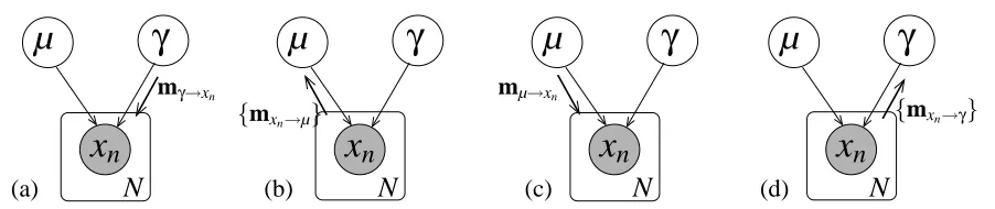
n

Figure 3: (a)-(d) Message passing procedure for variational inference in a univariate Gaussian model. The box around the xi node denotes a plate, which indicates that the contained

node and its connected edges are duplicated N times. The braces around the messages leaving the plate indicate that a set of N distinct messages are being sent.

=

−1

2(xn−µ)2 1 2

T _γ

lnγ

−ln 2π (22)

which shows that, for conjugacy, uµ(µ)must be[µ,µ2]T and uγ(γ)must be[γ,lnγ]T or linear

trans-forms of these.4 If we use a separate conjugate prior for each parameter then µ must have a Gaussian prior and γa gamma prior since these are the exponential family distributions with these natural statistic vectors. Alternatively, we could have chosen a normal-gamma prior over both parameters which leads to a slightly more complicated message passing procedure. We define the parameter priors to have hyper-parameters m,β, a and b, so that

ln P(µ|m,β) =

_β

m −β/2

T µ µ2

+1

2(lnβ−βm

2₋_{ln 2}_π₎

ln P(γ|a,b) =

−b a−1

T _γ

lnγ

+a ln b−lnΓ(a).

3.4.1 VARIATIONALMESSAGEPASSING IN THEUNIVARIATE GAUSSIANMODEL

We can now apply variational message passing to infer the distributions over µ andγvariationally. The variational distribution is fully factorised and takes the form

Q(µ,γ) =Qµ(µ)Qγ(γ).

We start by initialising Qµ(µ)and Qγ(γ) and find initial values ofhuµ(µ)iandhuγ(γ)i. Let us

choose to update Qµ(µ) first, in which case variational message passing will proceed as follows

(illustrated in Figure 3a-d).

(a) As we wish to update Qµ(µ), we must first ensure that messages have been sent to the children

of µ by any co-parents. Thus, messages mγ→xn are sent fromγto each of the observed nodes

xn. These messages are the same, and are just equal to huγ(γ)i= [hγi,hlnγi]T, where the

expectation are with respect to the initial setting of Qγ.

(12)

(b) Each xnnode has now received messages from all co-parents of µ and so can send a message

to µ which is the expectation of the natural parameter vector in (21),

mxn→µ=

hγixn −hγi/2

.

(c) Node µ has now received its full complement of incoming messages and can update its natural parameter vector,

φ∗ µ=

_β

m −β/2

+

N

∑

n=1

mxn→µ.

The new expectationhuµ(µ)i can then be computed under the updated distribution Q∗µ and

sent to each xnas the message mµ→xn= [hµi,hµ

2_i_]T_.

(d) Finally, each xnnode sends a message back toγwhich is

mxn→γ=

−1 2(x

2

n−2xnhµi+hµ2i) 1

2

andγcan update its variational posterior

φ∗

γ =

−b a−1

+

N

∑

n=1

mxn→γ.

As the expectation of u_γ(γ) has changed, we can now go back to step (a) and send an updated message to each xn node and so on. Hence, in variational message passing, the message passing

procedure is repeated again and again until convergence (unlike in belief propagation on a junction tree where the exact posterior is available after a message passing is performed once). Each round of message passing is equivalent to one iteration of the update equations in standard variational inference.

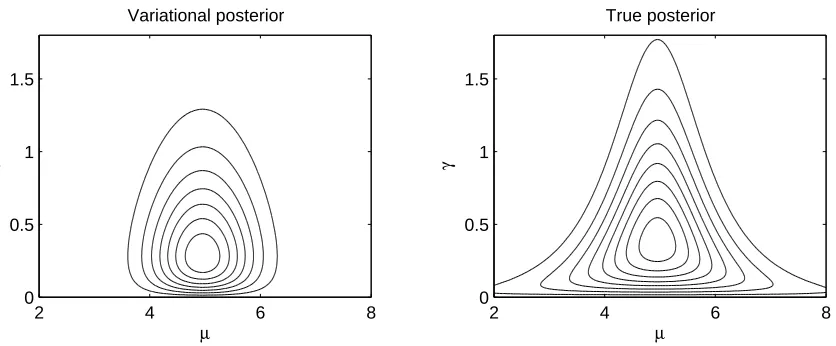
Figure 4 gives an indication of the accuracy of the variational approximation in this model, showing plots of both the true and variational posterior distributions for a toy example. The differ-ence in shape between the two distributions is due to the requirement that Q be factorised. Because KL(Q||P)has been minimised, the optimal Q is the factorised distribution which lies slightly inside P.

3.5 Initialisation and Message Passing Schedule

The variational message passing algorithm is guaranteed to converge to a local minimum of the KL divergence. As with many approximate inference algorithms, including Expectation-Maximisation and Expectation Propagation, it is important to have a good initialisation to ensure that the local minimum that is found is sufficiently close to the global minimum. What makes a good initialisation will depend on the model. In some cases, initialising each factor to a broad distribution will suffice, whilst in others it may be necessary to use a heuristic, such as using K-means to initialise a mixture model.

(13)

2 4 6 8 0

0.5 1 1.5

µ

γ

Variational posterior

2 4 6 8

0 0.5 1 1.5

True posterior

µ

γ

Figure 4: Contour plots of the variational and true posterior over the mean µ and precision γof a Gaussian distribution, given four samples from

N

(x|5,1). The parameter priors are

P(µ) =

N

(0,1000)and P(γ) =Gamma(0.001,0.001).

messages in VMP can be passed according to a very flexible schedule. At any point, any factor can be selected and it can be updated locally using only messages from its neighbours and co-parents. There is no requirement that factors be updated in any particular order. However, changing the up-date order can change which stationary point the algorithm converges to, even if the initialisation is unchanged.

Another constraint on belief propagation is that it is only exact for graphs which are trees and suffers from double-counting if loops are included. VMP does not have this restriction and can be applied to graphs of general form.

3.6 Calculation of the Lower Bound

L

(Q)

The variational message passing algorithm makes use of the lower bound

L

(Q)as a diagnostic of convergence. Evaluating the lower bound is also useful for performing model selection, or model averaging, because it provides an estimate of the log evidence for the model.

The lower bound can also play a useful role in helping to check the correctness both of the ana-lytical derivation of the update equations and of their software implementation, simply by evaluating the bound after updating each factor in the variational posterior distribution and checking that the value of the bound does not decrease. This can be taken a stage further (Bishop and Svens´en, 2003) by using numerical differentiation applied to the lower bound. After each update, the gradient of the bound is evaluated in the subspace corresponding to the parameters of the updated factor, to check that it is zero (within numerical tolerances). This requires that the differentiation take account of any constraints on the parameters (for instance that they be positive or that they sum to one). These checks, of course, provide necessary but not sufficient conditions for correctness. Also, they add computational cost so would typically only be employed whilst debugging the implementation.

(14)

Although the correctness tests discussed above also provide a check on the mutual consistency of the two bodies of code, it would clearly be more elegant if their evaluation could be unified.

This is achieved naturally in the variational message passing framework by providing a way to calculate the bound automatically, as will now be described. To recap, the lower bound on the log evidence is defined to be

L

(Q) =hln P(H,V)i − hln Q(H)i,

where the expectations are with respect to Q. In a Bayesian network, with a factorised Q distribution, the bound becomes

L

(Q) =

∑

i

hln P(Xi|pai)i −

∑

i∈H

hln Qi(Hi)i

def

=

∑

i

L

i

where it has been decomposed into contributions from the individual nodes{

L

i}. For a particular

latent variable node Hj, the contribution is

L

j=

ln P(Hj|paj)

−ln Qj(Hj)

.

Given that the model is conjugate-exponential, we can substitute in the standard form for the expo-nential family

L

j = hφj(paj)Tihuj(Hj)i+hfj(Hj)i+hgj(paj)i −hφ∗_jThuj(Hj)i+hfj(Hj)i+gej(φ∗j)

i

,

where the functiongejis a reparameterisation of gjso as to make it a function of the natural parameter

vector rather than the parent variables. This expression simplifies to

L

j = (hφj(paj)i −φ∗j) T

huj(Hj)i+hgj(paj)i −gej(φ∗j). (23)

Three of these terms are already calculated during the variational message passing algorithm:hφ_j(paj)i

andφ∗_j when finding the posterior distribution over Hj in (20), andhuj(Hj)iwhen calculating

out-going messages from Hj. Thus, considerable saving in computation are made compared to when

the bound is calculated separately.

Each observed variable Vkalso makes a contribution to the bound

L

k = hln P(Vk|pak)i

= hφ_k(pak)iTuk(Vk) +fk(Vk) +gek(hφk(pak)i).

Again, computation can be saved by computing uk(Vk) during the initialisation of the message

passing algorithm.

Example 1 Calculation of the Bound for the Univariate Gaussian Model

In the univariate Gaussian model, the bound contribution from each observed node xnis

L

xn =

hγihµi −hγi/2

T xn x2_n

+1

2 hlnγi − hγihµ

(15)

and the contributions from the parameter nodes µ andγare

L

µ =

_β

m−β0m0 −β/2+β0/2

T hµi hµ2i

+1

2 lnβ−βm

2₋_ln_β0₊_β0_m02

L

γ =

−b+b0 a−a0

T hγi hlnγi

+a ln b−lnΓ(a)−a0ln b0+lnΓ(a0).

The bound for this univariate Gaussian model is given by the sum of the contributions from the µ andγnodes and all xnnodes.

4. Allowable Models

The variational message passing algorithm can be applied to a wide class of models, which will be characterised in this section.

4.1 Conjugacy Constraints

The main constraint on the model is that each parent–child edge must satisfy the constraint of conjugacy. Conjugacy allows a Gaussian variable to have a Gaussian parent for its mean and we can extend this hierarchy to any number of levels. Each Gaussian node has a gamma parent as the distribution over its precision. Furthermore, each gamma distributed variable can have a gamma distributed scale parameter b, and again this hierarchy can be extended to multiple levels.

A discrete variable can have multiple discrete parents with a Dirichlet prior over the entries in the conditional probability table. This allows for an arbitrary graph of discrete variables. A variable with an Exponential or Poisson distribution can have a gamma prior over its scale or mean respectively, although, as these distributions do not lead to hierarchies, they may be of limited interest.

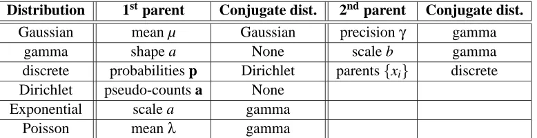
These constraints are listed in Table 1. This table can be encoded in implementations of the variational message passing algorithm and used during initialisation to check the conjugacy of the supplied model.

4.1.1 TRUNCATEDDISTRIBUTIONS

The conjugacy constraint does not put any restrictions on the fX(X)term in the exponential family

distribution. If we choose fX to be a step function

fX(X) =

0 : X≥0

−∞ : X<0

then we end up with a rectified distribution, so that P(X|θ) =0 for X <0. The choice of such a truncated distribution will change the form of messages to parent nodes (as the gX normalisation

(16)

Distribution 1stparent Conjugate dist. 2ndparent Conjugate dist.

Gaussian mean µ Gaussian precisionγ gamma

gamma shape a None scale b gamma

discrete probabilities p Dirichlet parents{xi} discrete

Dirichlet pseudo-counts a None

Exponential scale a gamma

Poisson meanλ gamma

Table 1: Distributions for each parameter of a number of exponential family distributions if the model is to satisfy conjugacy constraints. Conjugacy also holds if the distributions are replaced by their multivariate counterparts e.g. the distribution conjugate to the precision matrix of a multivariate Gaussian is a Wishart distribution. Where “None” is specified, no standard distribution satisfies conjugacy.

potential problem with the use of a truncated distribution is that no standard distributions may exist which are conjugate for each distribution parameter.

4.2 Deterministic Functions

We can considerably enlarge the class of tractable models if variables are allowed to be defined as deterministic functions of the states of their parent variables. This is achieved by adding determin-istic nodes into the graph, as have been used to similar effect in the BUGS software (see Section 5). Consider a deterministic node X which has stochastic parents Y={Y1, . . . ,YM}and which has

a stochastic child node Z. The state of X is given by a deterministic function f of the state of its parents, so that X= f(Y). If X were stochastic, the conjugacy constraint with Z would require that

P(X|Y) must have the same functional form, with respect to X , as P(Z|X). This in turn would dictate the form of the natural statistic vector uX of X , whose expectationhuX(X)iQwould be the

message from X to Z.

Returning to the case where X is deterministic, it is still necessary to provide a message to Z of the formhuX(X)iQwhere the function uX is dictated by the conjugacy constraint. This message

can be evaluated only if it can be expressed as a function of the messages from the parent variables, which are the expectations of their natural statistics functions {huYi(Yi)iQ}. In other words, there

must exist a vector functionψ_X such that

huX(f(Y))iQ=ψX(huY1(Y1)iQ, . . . ,huYM(YM)iQ).

As was discussed in Section 3.2, this constrains uX(f(Y))to be a multi-linear function of the set of

functions{uYi(Yi)}.

A deterministic node can be viewed as a having a conditional distribution which is a delta func-tion, so that P(X|Y) =δ(X−f(Y)). If X is discrete, this is the distribution that assigns probability one to the state X=f(Y)and zero to all other states. If X is continuous, this is the distribution with the property thatR

(17)

Example 2 Using a Deterministic Function as the Mean of a Gaussian

Consider a model where a deterministic node X is to be used as the mean of a child Gaussian distri-bution

N

(Z|X,β−1)and where X equals a function f of Gaussian-distributed variables Y1, . . . ,YM. The natural statistic vectors of X (as dictated by conjugacy with Z) and those of Y1, . . . ,YM are

uX(X) =

X X2

, uYi(Yi) =

Yi Y2

i

for i=1. . .M

The constraint on f is that uX(f) must be multi-linear in{uYi(Yi)}and so both f and f

2 _{must be} multi-linear in {Yi} and{Y_i2}. Hence, f can be any multi-linear function of Y1, . . . ,YM. In other words, the mean of a Gaussian can be the sum of products of other Gaussian-distributed variables.

Example 3 Using a Deterministic Function as the Precision of a Gaussian

As another example, consider a model where X is to be used as the precision of a child Gaussian distribution

N

(Z|µ,X−1)and where X is a function f of gamma-distributed variables Y1, . . . ,YM. The natural statistic vectors of X and Y1, . . . ,YM are

uX(X) =

X

ln X

, uYi(Yi) =

Yi

lnYi

for i=1. . .M.

and so both f and ln f must be multi-linear in{Yi}and{lnYi}. This restricts f to be proportional to a product of the variables Y1, . . . ,YM as the logarithm of a product can be found in terms of the logarithms of terms in that product. Hence f =c∏_iYiwhere c is a constant. A function containing a summation, such as f =∑_iYi, would not be valid as the logarithm of the sum cannot be expressed as a multi-linear function of Yiand lnYi.

4.2.1 VALIDATINGCHAINS OFDETERMINISTICFUNCTIONS

The validity of a deterministic function for a node X is dependent on the form of the stochastic nodes it is connected to, as these dictate the functions uX and{uYi(Yi)}. For example, if the function was a

summation f =∑_iYi, it would be valid for the first of the above examples but not for the second. In

addition, it is possible for deterministic functions to be chained together to form more complicated expressions. For example, the expression X=Y1+Y2Y3can be achieved by having a deterministic product node A with parents Y2 and Y3 and a deterministic sum node X with parents Y1 and A. In

this case, the form of the function uA is not determined directly by its immediate neighbours, but

instead is constrained by the requirement of consistency for the connected deterministic subgraph. In a software implementation of variational message passing, the validity of a particular deter-ministic structure can most easily be checked by requiring that the function uXi be specified

explic-itly for each deterministic node Xi, thereby allowing the existing mechanism for checking conjugacy

to be applied uniformly across both stochastic and deterministic nodes.

4.2.2 DETERMINISTICNODEMESSAGES

To examine message passing for deterministic nodes, we must consider the general case where the deterministic node X has multiple children{Zj}. The message from the node X to any child Zj is

simply

mX→Zj = huX(f(Y))iQ

(18)

For a particular parent Yk, the function uX(f(Y))is linear with respect to uYk(Yk)and so it can be

written as

uX(f(Y)) =ΨX,Yk({uYi(Yi)}i=k6 ).uYk(Yk) +λ({uYi(Yi)}i6=k)

whereΨX,Ykis a matrix function of the natural statistics vectors of the co-parents of Yk. The message

from a deterministic node to a parent Yk is then

mX→Yk =

"

∑

j

mZj→X

#

ΨX,Yk({mYi→X}i6=k)

which relies on having received messages from all the child nodes and from all the co-parents. The sum of child messages can be computed and stored locally at the node and used to evaluate all child-to-parent messages. In this sense, it can be viewed as the natural parameter vector of a distribution which acts as a kind of pseudo-posterior over the value of X .

4.3 Mixture Distributions

So far, only distributions from the exponential family have been considered. Often it is desirable to use richer distributions that better capture the structure of the system that generated the data. Mixture distributions, such as mixtures of Gaussians, provide one common way of creating richer probability densities. A mixture distribution over a variable X is a weighted sum of a number of component distributions

P(X| {πk},{θk}) = K

∑

k=1

πkPk(X|θk)

where each Pk is a component distribution with parameters θk and a corresponding mixing

coeffi-cientπk indicating the weight of the distribution in the weighted sum. The K mixing coefficients

must be non-negative and sum to one.

A mixture distribution is not in the exponential family and therefore cannot be used directly as a conditional distribution within a conjugate-exponential model. Instead, we can introduce an additional discrete latent variableλwhich indicates from which component distribution each data point was drawn, and write the distribution as

P(X|λ,{θk}) =

K

∏

k=1

Pk(X|θk)δλk.

Conditioned on this new variable, the distribution is now in the exponential family provided that all of the component distributions are also in the exponential family. In this case, the log conditional probability of X given all the parents (includingλ) can be written as

ln P(X|λ,{θk}) =

∑

k

δ(λ,k)φ_k(θk)Tuk(X) +fk(X) +gk(θk)

.

If X has a child Z, then conjugacy will require that all the component distributions have the same natural statistic vector, which we can then call uX so: u1(X) =u2(X) =. . .=uK(X)def=uX(X). In

(19)

the same form (that is, f1= f2=. . .= fK def

= fX), although this is not required by conjugacy. In this

case, where all the distributions are the same, the log conditional becomes

ln P(X|λ,{θk}) =

"

∑

k

δ(λ,k)φ_k(θk)

#T

uX(X) +fX(X)

+

∑

k

δ(λ,k)gk(θk)

= φ_X(λ,{θk})TuX(X) +fX(X) +geX(φX(λ,{θk}))

where we have defined φ_X =∑kδ(λ,k)φk(θk) to be the natural parameter vector of this mixture

distribution and the functiong_eX is a reparameterisation of gX to make it a function ofφX (as in

Section 3.6). The conditional is therefore in the same exponential family form as each of the com-ponents.

We can now apply variational message passing. The message from the node X to any child is

huX(X)ias calculated from the mixture parameter vectorφ_X(λ,{θk}). Similarly, the message from X to a parentθk is the message that would be sent by the corresponding component if it were not

in a mixture, scaled by the variational posterior over the indicator variable Q(λ=k). Finally, the message from X toλis the vector of size K whose kth element ishln Pk(X|θk)i.

4.4 Multivariate Distributions

Until now, only scalar variables have been considered. It is also possible to handle vector variables in this framework (or to handle scalar variables which have been grouped into a vector to capture posterior dependencies between the variables). In each case, a multivariate conditional distribution is defined in the overall joint distribution P and the corresponding factor in the variational posterior

Q will also be multivariate, rather than factorised with respect to the elements of the vector. To

understand how multivariate distributions are handled, consider the d-dimensional Gaussian distri-bution with mean µ and precision matrix5Λ:

P(x|µ,Λ−1) =

s

|Λ|

(2π)dexp −

1 2(x−µ)

T_Λ₍_x₋_µ₎_.

This distribution can be written in exponential family form

lnN(x|µ,Λ−1) =

_Λ

µ −1

2vec(Λ) T

x

vec(xxT)

+1

2(ln|Λ| −µ

T_Λ_µ₋_{d ln 2}_π₎

where vec(·) is a function that re-arranges the elements of a matrix into a column vector in some consistent fashion, such as by concatenating the columns of the matrix. The natural statistic function for a multivariate distribution therefore depends on both the type of the distribution and its dimen-sionality d. As a result, the conjugacy constraint between a parent node and a child node will also constrain the dimensionality of the corresponding vector-valued variables to be the same. Multi-variate conditional distributions can therefore be handled by VMP like any other exponential family distribution, which extends the class of allowed distributions to include multivariate Gaussian and Wishart distributions.

(20)

A group of scalar variables can act as a single parent of a vector-valued node. This is achieved using a deterministic concatenation function which simply concatenates a number of scalar values into a vector. In order for this to be a valid function, the scalar distributions must still be conjugate to the multivariate distribution. For example, a set of d univariate Gaussian distributed variables can be concatenated to act as the mean of a d-dimensional multivariate Gaussian distribution.

4.4.1 NORMAL-GAMMADISTRIBUTION

The mean µ and precision γparameters of a Gaussian distribution can be grouped together into a single bivariate variable c={µ,γ}. The conjugate distribution for this variable is the normal-gamma distribution, which is written

ln P(c|m,λ,a,b) =

   

mλ −1

2λ

−b−1 2λm

2 a−1

2    

   

µγ µ2γ

γ

lnγ

  

+12(lnλ−ln 2π) +a ln b−lnΓ(a).

This distribution therefore lies in the exponential family and can be used within VMP instead of separate Gaussian and gamma distributions. In general, grouping these variables together will im-prove the approximation and so increase the lower bound. The multivariate form of this distribution, the normal-Wishart distribution, is handled as described above.

4.5 Summary of Allowable Models

In summary, the variational message passing algorithm can handle probabilistic models with the following very general architecture: arbitrary directed acyclic subgraphs of multinomial discrete variables (each having Dirichlet priors) together with arbitrary subgraphs of univariate and mul-tivariate linear Gaussian nodes (having gamma and Wishart priors), with arbitrary mixture nodes providing connections from the discrete to the continuous subgraphs. In addition, deterministic nodes can be included to allow parameters of child distributions to be deterministic functions of parent variables. Finally, any of the continuous distributions can be singly or doubly truncated to restrict the range of allowable values, provided that the appropriate moments under the truncated distribution can be calculated along with any necessary parent messages.

This architecture includes as special cases models such as hidden Markov models, Kalman filters, factor analysers, principal component analysers and independent component analysers, as well as mixtures and hierarchical mixtures of these.

5. VIBES: An Implementation of Variational Message Passing

(21)

(a)

N

µ

γ

x

i

(b)

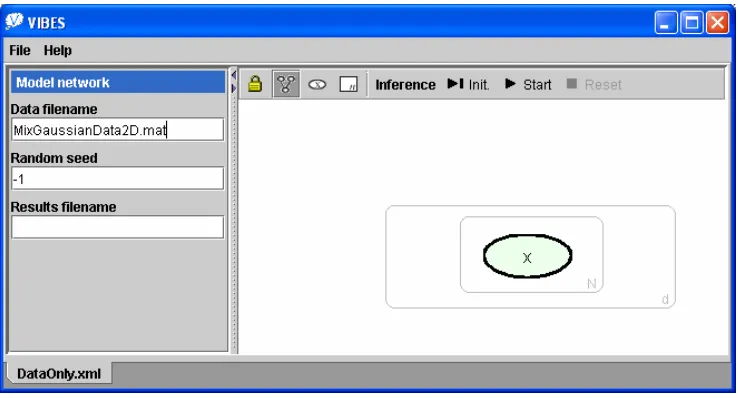
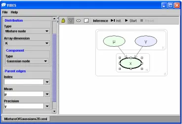
Figure 5: (a) Bayesian network for the univariate Gaussian model. (b) Screenshot of VIBES show-ing how the same model appears as it is beshow-ing edited. The node x is selected and the panel to the left shows that it has a Gaussian conditional distribution with mean µ and precisionγ. The plate surrounding x shows that it is duplicated N times and the heavy border indicates that it is observed (according to the currently attached data file).

VIBES. Models can also be specified in a text file, which contains XML according to a pre-defined model definition schema. VIBES is written in Java and so can be used on Windows, Linux or any operating system with a Java 1.3 virtual machine.

As in WinBUGS, the convention of making deterministic nodes explicit in the graphical rep-resentation has been adopted, as this greatly simplifies the specification and interpretation of the model. VIBES also uses the plate notation of a box surrounding one or more nodes to denote that those nodes are replicated some number of times, specified by the parameter in the bottom right hand corner of the box.

Once the model is specified, data can be attached from a separate data file which contains observed values for some of the nodes, along with sizes for some or all of the plates. The model can then be initialised which involves: (i) checking that the model is valid by ensuring that conjugacy and dimensionality constraints are satisfied and that all parameters are specified; (ii) checking that the observed data is of the correct dimensionality; (iii) allocating memory for all moments and messages; (iv) initialisation of the individual distributions Qi.

Following a successful initialisation, inference can begin immediately. As inference proceeds, the current state of the distribution Qi for any node can be inspected using a range of diagnostics

(22)

terminate automatically when the change in the bound during one iteration drops below a small value. Alternatively, the optimisation can be stopped after a fixed number of iterations.

The VIBES software can be downloaded from http://vibes.sourceforge.net. This soft-ware was written by one of the authors (John Winn) whilst a Ph.D. student at the University of Cambridge and is free and open source. Appendix A contains a tutorial for applying VIBES to an example problem involving a Gaussian Mixture model. The VIBES web site also contains an online version of this tutorial.

6. Extensions to Variational Message Passing

In this section, three extensions to the variational message passing algorithm will be described. These extensions are intended to illustrate how the algorithm can be modified to perform alternative inference calculations and to show how the conjugate-exponential constraint can be overcome in certain circumstances.

6.1 Further Variational Approximations: The Logistic Sigmoid Function

As it stands, the VMP algorithm requires that the model be conjugate-exponential. However, it is possible to sidestep the conjugacy requirement by introducing additional variational parameters and approximating non-conjugate conditional distributions by valid conjugate ones. We will now illustrate how this can be achieved using the example of a conditional distribution over a binary variable x∈0,1 of the form

P(x|a) = σ(a)x[1−σ(a)]1−x = eaxσ(−a)

where

σ(a) = 1

1+exp(−a)

is the logistic sigmoid function.

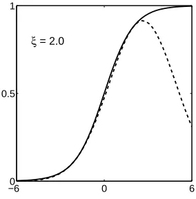
We take the approach of Jaakkola and Jordan (1996) and use a variational bound for the logistic sigmoid function defined as

σ(a)>F(a,ξ) def= σ(ξ)exp[(a−ξ)/2+λ(ξ)(a2−ξ2)]

whereλ(ξ) = [1/2−g(ξ)]/2ξandξis a variational parameter. For any given value of a we can make this bound exact by settingξ2=a2. The bound is illustrated in Figure 6 in which the solid curve shows the logistic sigmoid functionσ(a)and the dashed curve shows the lower bound F(a,ξ)

forξ=2.

We use this result to define a new lower bound

L

e 6

L

by replacing each expectation of the form hln[eaxσ(−a)]i with its lower bound hln[eaxF(−a,ξ)]i. The effect of this transformation is to replace the logistic sigmoid function with an exponential, therefore restoring conjugacy to the model. Optimisation of eachξparameter is achieved by maximising this new bound

L, leading to

e the re-estimation equation

ξ2₌_a2 Q.

(23)

−60 0 6 0.5

1

ξ = 2.0

Figure 6: The logistic sigmoid functionσ(a)and variational bound F(a,ξ).

It follows from (8) that the factor in Q corresponding to P(x|a)is updated using ln Q?_x(x) = hln(eaxF(−a,ξ))i_∼_Q_x_(x)+

∑

k∈chx

hln P(Xk|pak)i_∼_Q_x_(x)+const.

= haxi_∼_Q_x_(x)+

∑

k∈chx

hbkxi_∼Qx(x)+const.

= a?x+const.

where a?=hai+∑_khbkiand the{bk}arise from the child terms which must be in the form(bkx+

const.)due to conjugacy. Therefore, the variational posterior Qx(x)takes the form Qx(x) =σ(a?)x[1−σ(a?)]1−x.

6.1.1 USING THELOGISTICAPPROXIMATION WITHINVMP

We will now explain how this additional variational approximation can be used within the VMP framework. The lower bound

L

e contains terms likehln(eaxF(−a,ξ))iwhich need to be evaluated and so we must be able to evaluate [hai a2]T_{. The conjugacy constraint on a is therefore that}

its distribution must have a natural statistic vector ua(a) = [a a2]. Hence it could, for example, be

Gaussian.

For consistency with general discrete distributions, we write the bound on the log conditional ln P(x|a)as

ln P(x|a) >

0

a

T _δ (x−0)

δ(x−1)

+ (−a−ξ)/2+λ(ξ)(a2−ξ2) +lnσ(ξ)

=

_δ

(x−1)−1 2

λ(ξ)

T a a2

−ξ/2−λ(ξ)ξ2+lnσ(ξ).

The message from node x to node a is therefore

mx→a=

hδ(x−1)i −1 2

λ(ξ)

(24)

can be carried out, for example, just before sending a message from x to a. The only remaining modification is to the calculation of the lower bound in (23), where the termgj(paj)

is replaced by the expectation of its bound,

gj(paj)

>(− hai −ξ)/2+λ(ξ)(a2−ξ2) +lnσ(ξ).

This extension to VMP enables discrete nodes to have continuous parents, further enlarging the class of allowable models. In general, the introduction of additional variational parameters enor-mously extends the class of models to which VMP can be applied, as the constraint that the model distributions must be conjugate no longer applies.

6.2 Finding a Maximum A Posteriori Solution

The advantage of using a variational distribution is that it provides a posterior distribution over latent variables. It is, however, also possible to use VMP to find a Maximum A Posteriori (MAP) solution, in which values of each latent variable are found that maximise the posterior probability. Consider choosing a variational distribution which is a delta function

QMAP(H) =δ(H−H?)

where H?is the MAP solution. From (3), the lower bound is

L

(

Q

) = hln P(H,V)i − hln Q(H)i

= ln P(H?,V) +h_δ

where h_δis the differential entropy of the delta function. By considering the differential entropy of a Gaussian in the limit as the variance goes to 0, we can see that h_δ=log a,a→0. Thus h_δ does not depend on H? and so maximising

L

(

Q

)is equivalent to finding the MAP solution. However, since the entropy h_δtends to−∞, so does

L

(

Q

)and so, whilst it is still trivially a lower bound on the log evidence, it is not an informative one. In other words, knowing the probability density of the posterior at a point is uninformative about the posterior mass.

The variational distribution can be written in factorised form as

QMAP(H) =

∏

j

Qj(Hj).

with Qj(Hj) =δ(Hj−H?j). The KL divergence between the approximating distribution and the true

posterior is minimised if KL(Qj||Q?j) is minimised, where Q?j is the standard variational solution

given by (6). Normally, Qj is unconstrained so we can simply set it to Q?j. However, in this case, Qjis a delta function and so we have to find the value of H?j that minimises KL(δ(Hj−H?j)||Q?j).

Unsurprisingly, this is simply the value of H?_j that maximises Q?_j(H?_j).

In the message passing framework, a MAP solution can be obtained for a particular latent vari-able Hjdirectly from the updated natural statistic vectorφ?j using

(φ?_j)Tduj(Hj) dHj

=0.

For example, if Q?_j is Gaussian with mean µ then H?_j =µ or if Q?_j is gamma with parameters a,b,

(25)

Given that the variational posterior is now a delta function, the expectation of any function

hf(Hj)iunder the variational posterior is just f(H?j). Therefore, in any outgoing messages,huj(Hj)i

is replaced by uj(H?j). Since all surrounding nodes can process these messages as normal, a MAP

solution may be obtained for any chosen subset of variables (such as particular hyper-parameters), whilst a full posterior distribution is retained for all other variables.

6.3 Learning Non-conjugate Priors by Sampling

For some exponential family distribution parameters, there is no standard probability distribution which can act as a conjugate prior. For example, there is no standard distribution which can act as a conjugate prior for the shape parameter a of the gamma distribution. This implies that we cannot learn a posterior distribution over a gamma shape parameter within the basic VMP framework. As discussed above, we can sometimes introduce conjugate approximations by adding variational parameters, but this may not always be possible.

The purpose of the conjugacy constraint is two-fold. First, it means that the posterior distri-bution of each variable, conditioned on its neighbours, has the same form as the prior distridistri-bution. Hence, the updated variational distribution factor for that variable has the same form and inference involves just updating the parameters of that distribution. Second, conjugacy results in variational distributions being in standard exponential family form allowing their moments to be calculated analytically.

If we ignore the conjugacy constraint, we get non-standard posterior distributions and we must resort to using sampling or other methods to determine the moments of these distributions. The disadvantages of using sampling include computational expense, inability to calculate an analytical lower bound and the fact that inference is no longer deterministic for a given initialisation and ordering. The use of sampling methods will now be illustrated by an example showing how to sample from the posterior over the shape parameter of a gamma distribution.

Example 4 Learning a Gamma Shape Parameter

Let us assume that there is a latent variable a which is to be used as the shape parameter of K gamma distributed variables{x1. . .xK}. We choose a to have a non-conjugate prior of an inverse-gamma distribution:

P(a|α,β)∝a−α−1exp

−β a

.

The form of the gamma distribution means that messages sent to the node a are with respect to a natural statistic vector

ua=

a

lnΓ(a)

which means that the updated factor distribution Q?_ahas the form

ln Q?_a(a) =

"

K