A Compression Approach to Support Vector Model Selection

(1)

A Compression Approach to Support Vector Model Selection

Ulrike von Luxburg [email protected]

Olivier Bousquet [email protected]

Bernhard Sch¨olkopf [email protected]

Max Planck Institute for Biological Cybernetics Spemannstrasse 38

72076 T¨ubingen, Germany

Editor: John Shawe-Taylor

Abstract

In this paper we investigate connections between statistical learning theory and data compression on the basis of support vector machine (SVM) model selection. Inspired by several generalization bounds we construct “compression coefficients” for SVMs which measure the amount by which the training labels can be compressed by a code built from the separating hyperplane. The main idea is to relate the coding precision to geometrical concepts such as the width of the margin or the shape of the data in the feature space. The so derived compression coefficients combine well known quantities such as the radius-margin term R2/ρ2_{, the eigenvalues of the kernel matrix, and}

the number of support vectors. To test whether they are useful in practice we ran model selection experiments on benchmark data sets. As a result we found that compression coefficients can fairly accurately predict the parameters for which the test error is minimized.

Keywords: Support vector machine, compression coefficient, minimum description length, model

selection

1. Introduction

In classification one tries to learn the dependency of labels y on patterns x from a given training set

(xi,yi)i=1...m. We are interested in the connections between two different methods to analyze this

problem: a data compression approach and statistical learning theory.

The minimum description length (MDL) principle (cf. Barron et al., 1998, and references therein) states that, among a given set of hypotheses, one should choose the hypothesis that achieves the shortest description of the training data. Intuitively, this seems to be a reasonable choice: by Shan-non’s source coding theorem (cf. Cover and Thomas, 1991) we know that an efficient code is closely related to the data generating distribution. Moreover, an easy-to-describe hypothesis is less likely to overfit than a more complicated one.

(2)

space, it bounds the generalization error essentially by the quantity −ln P(U)/m, where U is the subset of hypotheses consistent with the training examples. Intuitively we can argue that, according

to Shannon’s theorem,₋ln P(U)corresponds to the length of the shortest code for this subset.

There are statistical learning theory approaches which directly use compression arguments to bound the generalization ability of a classifier, for example the one of Vapnik (1998, sec. 6.2). In this framework, classifiers are used to construct codes that can transmit the labels of a set of training patterns. What those codes essentially do is to tell the receiver which classifier h from a given hypotheses class he should use to reconstruct the training labels from the training patterns (this is

described in detail in Section 2). For such a code, the compression coefficient C(h)is defined as

C(h):= number of bits to code y1, ...,ymusing h

m . (1)

The denominator corresponds to the number of bits we need to transmit the uncompressed binary

vector(y1, ...,ym). The numerator tells us how many bits we need to transmit the same information

using the code constructed with help of classifier h. Hence, the compression coefficient is a number between 0 and 1 which describes how efficient the code works. Intuitively, if the compression

coefficient C(h) is small, h is a “simple” hypothesis which we expect not to overfit too much and

hence to have a small generalization error. This belief is supported by the following theorem, which

bounds the risk R(h) of a classifier h (i.e., the expected generalization error with respect to the

0-1-loss) in terms of the compression coefficient:

Theorem 1 (Section 6.2 in Vapnik 1998) With probability at least 1₋ηover m random training points drawn iid according to the unknown distribution P, the risk R(h)of classifier h is bounded by

R(h)_≤2 ln(2)C(h)₋ln(η)

m

simultaneously for all classifiers h in a finite hypotheses set.

This bound has the disadvantage that it is only valid in the restricted setting where the hypotheses space is finite and independent of the training data.

A different bound that directly works in the coding setting has recently been stated by Blum and Langford (2003). Their setting is slightly different from the one of Vapnik. For a given set of

training and test points, the sender constructs a codeσthat transmits the labels of both training and

test points. Rtestis then defined as the error which the codeσmakes on the given test set.

Theorem 2 (Corollary 3 in Blum and Langford 2003) With probability at least 1−ηover m ran-dom training points and m ranran-dom test points drawn iid according to the unknown distribution P, and for all codesσwhich encode the training labels without error, the error Rtest(σ)on the test set

satisfies

Rtest(σ)_≤C(σ)₋lnη

m .

(3)

Inspired by the compression coefficient bounds we want to explore whether the connection between statistical learning theory and data compression is only of theoretical interest or whether it can also be exploited for practical purposes. The first part of the work (Section 2) will consist in using hyperplanes learned by SVMs to construct codes for the training labels. Those codes work by encoding the direction of the separating hyperplane. To make them efficient, we will use geometric concepts such as the size of the margin or the shape of the data in the feature space, and sparsity arguments. The main insight of this section is on how to transform those geometrical concepts into an actual code for labels. In the end we obtain compression coefficients that contain quantities already known to be meaningful in the statistical learning theory of SVMs, such as the radius-margin

term R2/ρ2_{, the eigenvalues of the kernel matrix, and the number of support vectors. In the second}

part (Section 3) we then test the model selection performance of our compression coefficients on benchmark data sets. We find that the compression coefficients perform comparable or better than several standard bounds.

Now we want to establish some notation. We assume that the reader is familiar with some basic concepts concerning support vector machines such as a kernel, the margin, and support vectors. In

the following, the training data will always consist of m pairs(xi,yi)i=1,...,mof patterns with labels.

The patterns are assumed to live in some Hilbert space (the feature space), and the labels have binary

values_±1. For a given kernel function k we denote the kernel matrix by K := (k(xi,xj))i,j=1,...,m. We

will denote its eigenvalues byλ1, ...,λm, where theλi are sorted in non-increasing order. Later on

we will also consider the kernel matrix KSV restricted to the span of the support vectors. To define

it, let _{xi1, ...,xis} ⊂ {x1, ...,xm} the set of support vectors, SV :={k|xk ∈span{xi1, ...,xis}} the

indices of those training points which are in the subspace spanned by the support vectors. Then the

kernel matrix restricted to the span of the support vectors is defined as KSV:= (k(xi,xj))i,j∈SV. In the

MDL literature, classifiers are called “hypotheses”. In what follows, we use the word “hypothesis” synonymous to “classifier”. A hypotheses space is then the space of all possible classifiers we can

choose from. The sphere Sd_R−1is the surface of a ball with radius R in the space d. The function log

will always denote the logarithm to the base 2. Code lengths will often be given by some logarithmic

term, for instance_dlog m_e. To keep the notations simple, we will omit the ceil brackets and simply

write log m.

2. Compression Coefficients for SVMs

The basic setup for the compression coefficient framework is the following. We are given m pairs

(xi,yi)i=1,...,mof training patterns with labels and assume that an imaginary sender and receiver both

know the training patterns. It will be the task of the sender to transmit the labels of the training patterns to the receiver. This reflects the basic structure of a classification problem: we want to

predict the labels y for given patterns x. That is, we want to learn something about P(y_|x). Sender

and receiver are allowed to agree on the details of the code before transmission starts. Then the sender gets the training data and chooses a classifier that separates the training data. He transmits to the receiver which classifier he chose. The receiver can then apply this classifier to the training patterns and reconstruct all the labels.

To understand how this works let us consider a simple example. Before knowing the data, sender

and receiver agree on a finite hypotheses space containing k hypotheses h1, ...,hk. The sender gets

(4)

hypotheses, say h7, classifies all training points correctly. In this case the sender transmits “7” to

the receiver. The receiver can now reconstruct the labels of the training patterns by classifying them

according to hypothesis h7. Now consider the case where there is no hypothesis that classifies all

training patterns correctly. In this case, the receiver cannot reconstruct all labels without error if the sender only transmits the hypothesis. Additionally he has to know which of the training points are misclassified by this hypothesis. In our example, assume that hypothesis 7 misclassifies the training points 3, 14, and 20. The information the sender now transmits is “hypothesis: 7; misclassified

points: 3, 14, 20”. The receiver can then construct the labels of all patterns according to h7 and

flip the labels he obtained for patterns 3, 14, and 20. After this, he has labeled all training patterns correctly.

This example shows how a classification hypothesis can be used to transmit the labels of training points. In general, a finite, fixed hypothesis space as it was used in the example may not contain a good hypothesis for previously unseen training points and will result in long codes. To avoid this, the sender will have to adapt the hypothesis space to the training points and communicate this to the receiver.

One principle that can already be observed in the example above is the way training errors are handled. As above, the code will always consist of two parts: the first part which serves to describe the hypothesis, and the second part, which tells the receiver which of the training points are misclassified by this hypothesis.

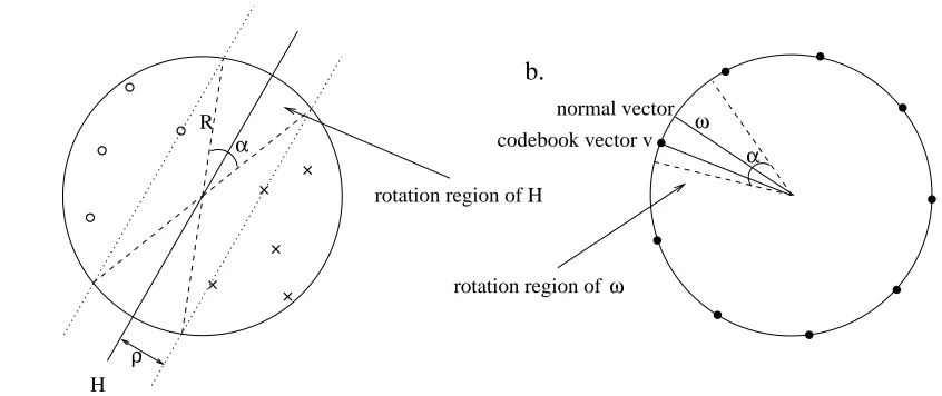
In the following we want to investigate how SVMs can be used for coding the labels. The main part of those codes will consist in transmitting the direction of the separating hyperplane constructed by the SVM. We will always consider the simplified problem where the hyperplane goes through the origin. The hypotheses space consists of all possible directions the normal vector can take. It can be identified with the unit sphere in the feature space. In case of an infinite dimensional feature space, recall that by the representer theorem the solution of an SVM always lies in the subspace spanned by the training points. Thus the normal vector we want to code is a vector in a Hilbert space of dimension at most m (where m is the number of training points). The trick to determine the precision by which we have to code this vector is to interpret the margin in terms of coding

precision: Suppose the data are (correctly) classified by a hyperplane with normal vector ω and

marginρ. A fact that often has been observed (e.g., Sch ¨olkopf and Smola, 2002, p. 194) is that in

case of a large margin, small perturbations of the direction of the hyperplane will not change the classification result on the training points. In compression language this means that we do not have to code the direction of the hyperplane with high accuracy – the larger the margin, the less accurate we have to code. So we will adapt the precision by which we code this direction to the width of the margin. Suppose that all training patterns lie in a ball of radius R around the origin and that

they are separated by a hyperplane H through the origin with normal vectorωand marginρ. Then

every “slightly rotated” hyperplane that still lies within the margin achieves the same classification result on all training points as the original hyperplane (cf. Figure 1a). Thus, instead of using the

hyperplane with normal vectorωto separate the training points we could use any convenient vector

v as normal vector – as long as the corresponding hyperplane still remains inside the margin. In this

context, note that rotating a hyperplane by some angleαcorresponds to rotating its normal vector

by the same angle. We denote the set of normal vectors such that the corresponding hyperplanes still

lie inside the margin the rotation region ofω. The region in which the corresponding hyperplanes

(5)

H

R

α

ρ

a.

rotation region of H

ω α

ω b.

rotation region of normal vector

codebook vector v

Figure 1: (a) The training points are separated by hyperplane H with marginρ. If we change the

direction of H such that the new hyperplane still lies inside the rotation region determined by the margin (dashed lines), the new hyperplane obtains the same classification result on the training points as H. (b) The hyperplanes in the rotation region of H (indicated by

the dashed lines) correspond to normal vectors inside the rotation region ofω. The black

points indicate the positions of equidistant codebook vectors on the sphere. The distance

between those vectors has to be chosen so small that in each cone of angleαthere is at

least one codebook vector. In this example, vector v is the codebook vector closest to

normal vectorω, and by construction it lies inside the rotation region ofω.

To code the direction ofω, we will construct a discrete set of “codebook vectors” on the sphere.

An arbitrary vector will be coded by choosing the closest codebook vector. From the preceding discussion we can see that the set of codebook vectors has to be constructed in such a way that the

closest codebook vector for every possible normal vectorω is inside the rotation region ofω(cf.

Figure 1b). An equivalent formulation is to construct a set of points on the surface of the sphere

such that the balls of radiusρcentered at those points cover the sphere. The minimal number of

balls we need to achieve this is called the covering number of the sphere.

Proposition 3 (Covering numbers of spheres) The number nd of balls of radiusρwhich are

re-quired to cover the sphere Sd_R−1of radius R in d-dimensional Euclidean space (d_≥2) satisfies

R ρ

d−1

≤nd≤2

Rπ

ρ d−1

.

The constant in the upper bound can be improved, but as we will be interested in log-covering numbers later, this does not make much difference in our application.

Proof We prove the upper bound by induction. For d =2, the sphere is a circle which can be

covered with_d2Rπ/ρ_{e ≤}2_dRπ/ρ_eballs. Now assume the proposition is true for the sphere Sd_R−1.

To construct aρ-covering on Sd_R we first cover the cylinder Sd_R−1_×[₋Rπ/2,Rπ/2]with a grid of

˜

(6)

sphere such that the one edge of the cylinder is mapped on the north pole, the other edge on the south pole, and the ’equator’ of the cylinder is mapped to the equator of the sphere. As the distances

between the grid points do not increase by this mapping, the projected points form aρ-cover of the

sphere Sd_R. By the induction assumption, the number of points in thisρ-cover satisfies

nd+1≤n˜d+1=nd· dRπ/ρe ≤2dRπ/ρed−1· dRπ/ρe=2dRπ/ρed.

We construct a lower bound on the covering number by dividing the surface area of the whole sphere by the area of the part of the surface covered by one single covering ball. The area of this part is smaller than the whole surface of the small ball. So we get a lower bound by dividing the

sur-face area of Sd_R−1by the surface area of Sd_ρ−1. As the surface area of a sphere with radius R is Rd−1

times the surface area of the unit sphere we get(R/ρ)d−1_{as lower bound for the covering number.}

Now we can explain how the sender will encode the direction of the separating hyperplane. Before getting the data, sender and receiver agree on a procedure on how to determine the centers of a covering of a unit sphere, given the number of balls to use for this covering, and on a way of enumerating these centers in some order. Furthermore, they agree on which kernel the sender will use for his SVM. Both sender and receiver get to see the training patterns, the sender also gets the training labels. Now the sender trains a (soft margin) SVM on the training data to obtain a

hyperplane that separates the training patterns with some marginρ(maybe with some errors). Then

he computes the number n of balls of radius ρone needs to cover the unit sphere in the feature

space according to Proposition 3. He constructs such a covering according to the procedure he and the receiver agreed on. The centers of the covering balls form his set of codebook vectors. The sender enumerates the set of codebook vectors in the predefined way from 1 to n. Then he chooses a codebook vector which lies inside the rotation region of the normal vector (this is always possible by

construction). We denote its index in∈ {1, ...,n}. Now he transmits the total number n of codebook

vectors and the index inof the one he chose. The receiver now constructs the same set of codebook

vectors according to the common procedure, enumerates them in the same predefined way as the

sender and picks vector in. This is the normal vector of the hyperplane he was looking for, and he

can now use the corresponding hyperplane to classify the training patterns. In the codes below, we

refer to the pair(n,in)as position of the codebook vector.

When we count how many bits the sender needs to transmit the two numbers n and inwe have

to keep in mind that to decode, the receiver has to know which parts of the binary string belong to n

and in, respectively. The number n of codebook vectors is given as in Proposition 3, but as it depends

on the margin it cannot be bounded independent from the training data. So the sender cannot use a fixed number of bits to encode n. Instead we use a trick described in Cover and Thomas (1991, p. 149): To build a code for the number n, we take the binary representation of n and duplicate every bit. To mark the end of the code we use the string 01. As an example, n = 27 with the binary representation 11011 will be coded as 111100111101. So the receiver knows that the code of n is finished when he comes upon a pair of nonequal bits. We now apply this trick recursively: to code n, we first have to code the length log n of its binary code and then send the actual bits of the code of n. But instead of coding log n with the duplication code explained above, we can also first transmit the length log log n of the code of log n and then transmit the code of log n, and so on. At some point we stop this recursive procedure and code the last remaining number with the duplication

(7)

the sum continues until the last positive term (cf. p. 150 in Cover and Thomas, 1991). Having

transmitted n, we can send inwith log n bits, because inis a number between 1 and n and the sender

now already knows n. All in all, the sender needs log∗n+log n bits to transmit the position of the

codebook vector.

The second part of the code deals with transmitting which of the training patterns are misclas-sified by the hyperplane corresponding to the chosen codebook vector. We have to be careful how we define the misclassified training points in case of a soft margin SVM. For a soft margin SVM it is allowed that some training points lie inside the margin. For those training points which end up inside the rotation region of the hyperplane, our rotation argument breaks down. It cannot be guaranteed that when the receiver uses the hyperplane corresponding to the codebook vector, the points inside the rotation region are classified in the same way as the sender classified them with the original hyperplane. Thus the sender has to transmit which points are inside the rotation region, and he also has to send their labels. All other points can be treated more easily. The sender has to transmit which of the points outside the rotation region were misclassified. The receiver knows that those points will also be misclassified by his hyperplane, and he can flip their labels to get them right. Below we will refer to the part consisting of the information on the points inside the rotation region and on the misclassified points outside the rotation region as misclassification information.

The number r of points inside the rotation region is a number between 0 and m, thus we can transmit its binary representation using log m bits. After transmitting r, the receiver knows how

many training points lie inside the region, but not which of them. There are m_r

possibilities which of the training points are the points inside the rotation region. Before transmission, sender and

receiver agree on an ordering on those possibilities. Now the sender can transmit the index irof the

one that is the true one. As this is a number between 1 and m_r

, and as the receiver at this point

already knows r, this can be encoded with log m_rbits. Next the sender can use r bits to send the

labels of the r points inside the rotation region. Finally the sender has to transmit the number l of

misclassified training points outside the rotation region. It is a number between 1 and m₋r, thus we

can use log(m₋r)bits for this. To transmit which of the vectors are the misclassified ones, we send

the index il with log m−_lr

bits. All together, we need log m+log m_r+r+log(m₋r) +log m−_l r

bits to transmit the misclassification information. For simplicity, we bound this quantity from above

by(r+l+2)log m+r.

Now we can formulate our first code:

Code 1 Sender and receiver agree on the training patterns, a fixed kernel, and on a procedure for choosing the positions of t balls to cover the unit sphere in a d-dimensional Euclidean space. Now the sender trains an SVM with the fixed kernel on the training patterns, determines the size of the margin ρand the number n of balls he needs to cover the sphere up to the necessary accuracy according to Proposition 3. Furthermore, he determines which of the training patterns lie inside the rotation region and which patterns outside this region are misclassified by the SVM solution. Now he transmits

• the position of the codebook vector (log∗n+log n bits)

• the misclassification information ((r+l+2)log m+r bits )

(8)

constructs a hyperplane using this vector as normal vector. He classifies all training patterns ac-cording to this hyperplane, labels the points inside the rotation region as transmitted by the sender, and flips the labels of the misclassified training points outside the rotation region.

As defined in Equation (1), the compression coefficient of a code is given by the number of bits it needs to transmit all its information, divided by the number m of labels that were transmitted. Hence, according to our computations above, the compression coefficient of Code 1 is given by

C1=

1 m(log

∗_n₊_{log n}_{+ (}_r₊_l₊₂₎_{log m}₊_r₎

with n=2_dRπ/ρ_ed−1according to Proposition 3.

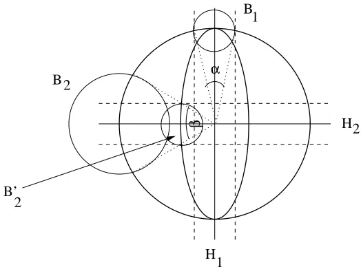
Now we want to refine this code in several aspects. In the construction above we worked with the smallest sphere which contains all the training points. But in practice, the shape of the data in the feature space is typically ellipsoid rather than spherical. This means that large parts of the sphere we used above are actually empty, and thus the code we constructed is not very efficient. Now we want to take into account the shape of the data in the feature space to construct a shorter code. In this setting it will turn out to be convenient to choose the hypotheses space to have the same shape as the data space. The reason for this is the following: When using the rotation argument from above, we observe that in the ellipsoid situation the maximal rotation angle of the hyperplane induced by

some fixed marginρdepends on the actual direction of the hyperplane (cf. Figure 2). This means

that the sets of points on a spherical hypotheses space which classify the training data in the same way as the hyperplane also have different sizes, depending on the direction of the hyperplane. To construct an optimal set of codebook vectors on the spherical hypotheses space we thus had to cover the sphere with balls of different sizes. Instead of this spherical hypotheses space now consider a hypotheses space which has the same ellipsoid form as the data space. In this case, the sets of vectors which correspond to directions inside the rotation regions can be represented by balls of equal sizes, centered on the surface of the ellipsoid (cf. Figure 2).

Now we want to determine the shape of the ellipsoid containing the data points in the feature space. The lengths of the principal axes of this ellipse can be described in terms of the eigenvalues of the kernel matrix:

Proposition 4 (Shape of the data ellipse) For given training patterns(xi)i=1,...,mand kernel k, let

λ1, ....,λdbe the eigenvalues of the kernel matrix K= (k(xi,xj))i,j=1,...,m. Then all training patterns

are contained in an ellipse with principal axes of lengths√λ1, ..., √_λ

din the feature space.

Proof The trick of the proof is to interpret the eigenvectors of the kernel matrix, who originally

live in d, as vectors in the feature space. Let Hm:=span{δxi|i=1, ...,m} the subspace of the

feature space spanned by the training examples. It is endowed with the scalar product_hδxi,δxjiK=

k(xi,xj). Let(ei)i=1,...,mthe canonical basis of mandh·,·i m the Euclidean scalar product. Define

the mapping T : m_→Hm,ei7→δxi. For u=∑

m

i=1uiei,v=∑mj=1vjej∈ mwe have

hTu,T v_iK=h m

∑

i=1

uiδxi, m

∑

j=1

vjδxjiK= m

∑

i,j=1

uivjhδxi,δxjiK= m

∑

i,j=1

uivjk(xi,xj) =u0Kv. (2)

Let v1, ...,vd∈ mbe the normalized eigenvectors of the matrix K corresponding to the eigenvalues

λ1, ...,λd, i.e., Kvi=λiviandhvi,vji m =δ_{i j}. From Equation (2) we can deduce

(9)

H 1

H2 B2

B 1

B’ 2

β

α

Figure 2: In this figure, the ellipse represents the data domain and the large circle represents a

spherical hypotheses space. Consider two hyperplanes H1 and H2 with equal margin.

The balls B1 resp. B2 indicate the sets of hypotheses that yield the same classification

result as H1resp. H2. The sizes of those balls depend on the direction of the hyperplane

with respect to the ellipse. In the example shown, B1is smaller than B2, hence H1must be

coded with higher accuracy than H2. Note that if we use the ellipse itself as hypotheses

space, we have to consider the balls B1 and B02 which are centered on the surface of the

ellipse and have equal size.

in particular_kT vikK =

√_λ

i. Furthermore we have

hδxi,T vjiK=hδxi, m

∑

l=1

(vj)lδxliK= m

∑

l=1

(vj)lk(xi,xl) = (Kvj)i= (λjvj)i=λj(vj)i.

Altogether we can now see that in the feature space, all data points δxi lie in the ellipse whose

principal axes have direction T vj and length

p

λj because the ellipse equation is satisfied:

d

∑

j=1





hδxi, T vj kT vjkKiK

p λj





2 =

∑

j

((vj)i)2≤1.

Here the last equality follows from the fact that∑j((vj)i)2is the Euclidean norm of a row vector of

the orthonormal matrix containing the eigenvectors(v1, ...,vd).

Now that we know the shape of the ellipse, we have to find out how many balls of radius ρ

(10)

high dimensional spaces this does not make much difference, especially if some of the axes are very small. Computing a rough bound on the covering numbers of an ellipse is easy:

Proposition 5 (Covering numbers of ellipses) The number n of balls of radius ρ which are re-quired to cover a d-dimensional ellipse with principal axes c1, ...,cd satisfies

d

∏

i=1

ci

ρ ≤n≤

d

∏

i=1

2ci

ρ

.

Proof The smallest parallelepiped containing the ellipse has side lengths 2c1, ...,2cd and can be

covered with a grid of∏d_i=1_d2ci/ρeballs of radius ρ. This gives an upper bound on the covering

number.

To obtain a lower bound we divide the volume of the ellipse by the volume of one single ball.

Let vd be the volume of a d-dimensional unit ball. Then the volume of a d-dimensional ball of

radiusρisρdvdand the volume of an ellipse with axes c1, ...,cdis given by vd∏di=1cd. So we need

at least∏d_i=1(ci/ρ)balls.

Now we can formulate the refined code:

Code 2 This code works analogously to Code 1, the only difference is that sender and receiver work with a covering of the data ellipse instead of a covering of the enclosing sphere.

The compression coefficient of Code 2 is

C2=

1 m(log

∗_n₊_{log n}_{+ (}_r₊_l₊₂₎_{log m}₊_r₎_,

with n=∏d_i=1_d2√λi/ρeaccording to Propositions 4 and 5.

It is interesting to notice that the main complexity term in the compression coefficient is the logarithm of the number of balls needed to cover the region of interest of the hypotheses space. So the shape of the bounds we obtain is very similar to classical bounds based on covering numbers in statistical learning theory. This is not so surprising since we explicitly approximate our hypotheses space by covers, but there is a somewhat deeper connection. Indeed, when we construct our code, we consider all normal vectors in a certain region as equivalent with respect to the labeling they give of the data. This means that we define a metric on the set of possible normal vectors which is related to the induced Hamming distance on the data (that is the natural distance in the ”coordinate projections” of our function class on the data). Hence, when we adapt the size of the balls to the direction in hypotheses space (in Figure 2), we actually say that Hamming distance 1 on the data translates into a certain radius. Hence, we are led to build covers in this induced distance which is exactly the distance which is used in classical covering number bounds for classification. So the compression approach gives another motivation, of information theoretic flavor, for considering that the right measure of the capacity of a function class is the metric entropy of its coordinate projections.

Both compression coefficients we derived so far implicitly depend on the dimension d of the

feature space in which we code the hyperplane. Above we always used d=m as the solution of

(11)

by working in this subspace. The procedure then works as follows: the sender trains the SVM and

determines the support vectors and the marginρ. The ellipse that we have to consider now is the

ellipse determined by the kernel matrix KSV restricted to the linear span of the support vectors (cf.

notations at the end of Section 1). The reason for this is that we are only interested in what happens if we slightly change the direction of the normal vector within the subspace spanned by the support vectors.

To let the receiver know the subspace he is working in, the sender has to transmit which of the training patterns are support vectors. This part of the code will be called support vector information. As the number s of support vectors is between 0 and m, the sender first codes s with log m bits and

then the index isof the actual support vectors among the m_s

possibilities with log m_sbits. So the

support vector information can be coded with log m+log m_s_≤(s+1)log m bits. After submitting

the information about the support vectors, the code proceeds analogously to Code 2.

Code 3 Sender and receiver agree on the training patterns, the kernel, and the procedure of cover-ing an ellipsoid. After traincover-ing an SVM, the sender transmits

• the support vector information ((s+1)log m bits),

• the position of the codebook vector (log∗n+log n bits),

• the misclassification information ((r+l+2)log m+r bits ).

To decode, the receiver constructs the hypotheses space consisting of the data ellipse projected on the subspace spanned by the support vectors. He covers this ellipse with n balls and chooses the vector representing the normal vector of the hyperplane. Then he labels the training patterns by first projecting them into the subspace and then classifying them according to the hyperplane. Finally, he deals with the misclassified training points as in the codes before.

The compression coefficient of Code 3 is given as

C3=

1 m(log

∗_n₊_{log n}_{+ (}_r₊_l₊_s₊₃₎_{log m}₊_r₎_,

with n_≤∏s_i=1_d2√γi/ρeaccording to Propositions 4 and 5. Hereγi denote the eigenvalues of the

restricted kernel matrix KSV.

A further dimension reduction can be obtained with the following idea: It has been empirically observed that on most data sets the axes of the data ellipse decrease fast for large dimensions. Once the axis in one direction is very small, we want to discard this dimension by projecting in a lower dimensional subspace using kernel principal component decomposition (cf. Sch ¨olkopf and Smola,

2002). A projection P will be allowed if the image P(ω) of the normal vectorωis still within the

rotation region induced by the marginρ. In this case we construct codebook vectors for P(ω)in

the lower dimensional subspace. We have to make sure that the vector representing P(ω)is still

contained in the original rotation region.

In more detail, this approach works as follows: First we train the SVM and get the normal

vectorωand marginρ. For convenience, we now normalize ωto length R byω0:=_||ω_ω_||R. After

normalizing, we know that a vector v still lies inside the rotation region if _kω0−vk ≤ρ. Now

(12)

the projection on the subspace spanned by the first dP eigenvectors. To determine whether we are

allowed to perform projection dPwe have to check whetherkP(ω0)−ω0k ≤ρ. If not, the hyperplane

corresponding to P(ω0)is not within the rotation region any more, and we are not allowed to make

this projection. Otherwise, we are still within the rotation region after projecting ω0, so we can

discard the last m₋dP dimensions. In this case, we call P a valid projection. We then can encode

the projected normal vector P(ω0)in an dP-dimensional subspace. As P(ω0)is not in the center of

the rotation region any more, we have to code its direction more precisely now. We have to ensure

that the codebook vector v for P(ω0) still is in the original rotation region, that is_kv₋ω0k ≤ρ.

Define

cP:=

1

ρkω0−P(ω0)k

(note that for a valid projection, cP ∈[0,1]), and choose the radius r of the covering balls as r=

ρq1₋c2

P. Then we have

kω0−vk2≤ kω0−P(ω0)k2+kP(ω0)−vk2≤c2Pρ2+ (1−c2P)ρ2=ρ2.

Thus the codebook vector v is still within the allowed distance ofω0.

All in all our procedure now works as follows: The sender trains an SVM. From now on he works in the subspace spanned by the support vectors only. In this subspace, he performs the PCA

and determines the smallest dPsuch that the projection on the subspace of dPdimensions is a valid

projection.The principal axes of the ellipse in the subspace are now given by the first dPeigenvalues

of the restricted kernel matrix KSV, and we have to construct a covering of this ellipse with covering

radius r=ρ

q

1₋c2_P. Then the code proceeds as before. The number dPwill be called the projection

information and can be encoded with log m bits.

Code 4 Sender and receiver agree on the training patterns, the kernel, the procedure of covering ellipsoids, and on how to perform kernel PCA. The sender trains the SVM and chooses a valid projection on some subspace. He transmits

• the projection information (log m bits),

• the position of the codebook vector (log∗n+log n bits),

• the misclassification information ((r+l+2)log m+r bits ).

To decode, the receiver constructs the hypotheses space consisting of the ellipse in the subspace spanned by the support vectors. Then he performs a PCA in this subspace and projects the hypothe-ses space on the subspace spanned by the first dP principal components. He covers the remaining

ellipse with n balls and continues as in the codes before.

The compression coefficient of this code is given by

C4=

1 m(log

∗_n₊_{log n}_{+ (}_r₊_l₊_s₊₄₎_{log m}₊_r₎_,

with n_≤∏dP

i=1d2√γi/(ρ

q

1₋c2_P)_e, cP as described above, andγi the eigenvalues of the restricted

(13)

So far we always considered codes which use the direction of the hyperplane as hypothesis. A totally different approach is to reduce the data by transmitting support vectors and their labels. Then the receiver can train his own SVM on the support vectors and will get the same result as the sender. Note that in this case, we not only have to transmit which of the vectors are support vectors as in the other codes, but also the labels of the support vectors. On the other hand we have the advantage that we do not have to treat the points inside the rotation region separately as they are support vectors anyway. The misclassification information only consists in the misclassified points which are not support vectors. This simple code works as follows:

Code 5 Sender and receiver agree on training patterns and a kernel. The sender sends

• the labels of the support vectors (s bits),

• the information on the misclassified points outside the rotation region ((l+1)log m bits).

To decode this information, the receiver trains an SVM with the support vectors as training set. Then he computes the classification result of this SVM for the remaining training patterns and flips the labels of the misclassified non-support vector training points.

This code has a compression coefficient of

C5=

1

m((s+l+2)log m+s).

3. Experiments

To test the utility of the derived compression coefficients for applications, we ran model selection experiments on different artificial and real world data sets. We used all data sets in the bench-mark data set repository compiled and explained in detail in R¨atsch et al. (2001). The data sets are available at http://ida.first.fraunhofer.de/projects/bench/benchmarks.htm. Most of the data sets in this repository are preprocessed versions of data sets originating from the UCI, Delve, or STATLOG repositories. In particular, all data sets are normalized. The data sets are called banana (5300 points), breast cancer (277 points), diabetis (768 points), flare-solar (1066 points), german (1000 points), heart (2700 points), image (2310 points), ringnorm (7400 points), splice (3175 points), thyroid (215 points), titanic (2201 points), twonorm (7400 points), waveform (5100 points). To be consistent with earlier versions of this manuscript we also used the data sets abalone (4177 points), Wisconsin breast cancer (683 points) from the UCI repository, and the US postal handwritten digits data set (9298 points). In all experiments, we first permuted the whole data set and divided it into as many

disjoint training subsets of sample size m=100 or 500 as possible. We centered each training subset

in the feature space as described in Section 14.2. of Sch ¨olkopf and Smola (2002) and then used it to train soft margin SVMs with Gaussian kernels. The test error was computed on the training subset’s complement.

For different choices of the soft margin parameter C _∈[100, ...,105] and the kernel width

σ∈[10−2_{, ...,}₁₀3_]_{we computed the compression coefficients and chose the parameters where the}

(14)

the origin. We compared the test errors corresponding to the chosen parameters to the ones obtained by model selection criteria from different generalization bounds. To state those bounds we denote

the empirical risk of a classifier by Remp and the true risk of a classifier by Rtrue. Note that the

definition of the risks varies slightly for the different bounds, for example with respect to the used loss function. We refer to the cited papers for details. The bounds we consider are the following:

• The radius-margin bound of Vapnik (1998). We here cite the version stated in Bartlett and

Shawe-Taylor (1999): with probability at least 1₋δ,

Rtrue≤Remp+

s c m(

R2

ρ2log

2_m₋_log_δ₎_.

The quantity we compute in the experiments is Remp+

p

(R2_{log m}₎_/₍ρ2_m₎_.

• The rescaled radius-margin bound of Chapelle and Vapnik (2000). It uses the shape of the

training data in the feature space to refine the classical radius margin bound. In this case, the

quantity R2/ρ2in the above bound is replaced by

m

∑

k=1

λ2 k max

i=1,...,mA 2 ik(

∑

j=1,...,m

Ajkyjαj)2,

where A is the matrix of the normalized eigenvectors of the kernel matrix K,λkare the

eigen-values of the kernel matrix, andαthe coefficients of the SVM solution.

• The trace bound of Bartlett and Mendelson (2001) which contains the eigenvalues of the

kernel matrix: with probability at least 1₋δ,

Rtrue≤Remp+Rademacher+

r

8 ln(2/δ)

m ,

where the Rademacher complexity is given by Rademacher_≤∑m_i=1pλi/m. The quantity we

compute in the experiments is Remp+Rademacher.

• The compression scheme bound of Floyd and Warmuth (1995) using the sparsity of the SVM

solution: with probability at least 1₋δ,

Rtrue≤

1 m₋s

ln

m

s

+lnm

2

δ

,

where s is the number of support vectors. In the experiments we computed the quantity

ln m_s/(m₋s). Note that if s=m this bound is infinite. We omitted those cases from the

plots.

• The sparse margin bound of Herbrich et al. (2000) which uses the size of the margin and the

sparsity of the solution: with probability at least 1₋δ,

Rtrue≤

1 m₋s

κlnem

κ +ln m2

δ

,

whereκ=min(_dR_ρ22+1e,d+1). For our experiments we compute the quantity

1 m₋s κln

em

κ

.

(15)

• The span estimate of Vapnik and Chapelle (2000), cf. also Opper and Winther (2000). This bound is different from all the other bounds as it estimates the leave-one-out error of the classifier. To achieve this, it bounds for each support vector how much the solution would change if this particular support vector were removed from the training set.

All experimental results shown below were obtained with training set size m=100; the results

for m=500 are comparable. The interested reader can study those results, as well as many

more plots which we cannot show here because they would use too much space, on the webpage http://www.kyb.tuebingen.mpg.de/bs/people/ule.

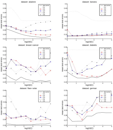
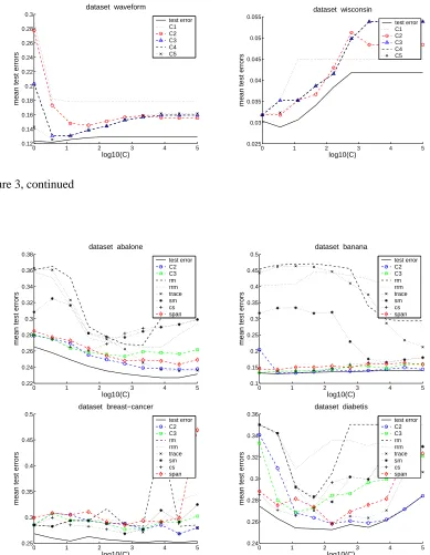
The goal of our first experiment is to use the compression coefficients to select the kernel width

σ. In Figure 3 we study which of the five compression coefficients achieves the best results on this

task. The plots in this figure were obtained as follows. For each training set, each parameter C and

each compression coefficient we chose the kernel widthσfor which the compression coefficient was

minimal. Then we evaluated the test error for the chosen parameters on the test set and computed the mean over all runs on the different training sets. Plotted are the means of these test errors versus parameter C, as well as the means of the minimal true test errors.

We can observe that for nearly all data sets, the compression coefficients C2, C3, and C4yield

better results than the simple coefficients C1 and C5. This can be explained by the fact that C1

and C5 only use one part of information (the size of the margin or the number of support vectors,

respectively), while the other coefficients combine several parts of information (margin, shape of

data, number of support vectors). When we compare coefficients C3and C4 we observe that they

have nearly identical values. This indicates that the gain we obtain by projecting into a smaller subspace using kernel PCA is outweighed by the additional information we have to transmit about

this projection. As C3 is simpler to compute, we thus prefer C3 to C4. From now on we want to

evaluate the results of the most promising compression coefficients C2and C3.

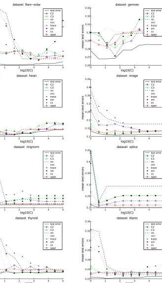
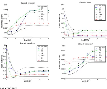
In Figure 4 we compare compression coefficients C2 and C3 to all the other model selection

criteria. The plots were obtained in the same way as the ones above. We see that for most data

sets, the performance of C2is rather good, and in most cases it is better than C3. It performs nearly

always comparable or better than the standard bounds, in particular it is nearly always better than

the widely-used radius margin bound. Among all bounds, C2and the span bound achieve the best

results. Comparing those two bounds shows that no one is superior to the other one: C2 is better

than the span bound on five data sets (abalone, banana, diabetis, german, usps), the span bound

is better than C2on five data sets (image, ringnorm, splice, thyroid, waveform), and they achieve

(16)

0 1 2 3 4 5 0.22

0.24 0.26 0.28 0.3 0.32 0.34 0.36 0.38

dataset abalone

log10(C)

mean test errors

test error C1 C2 C3 C4 C5

0 1 2 3 4 5

0.1 0.15 0.2 0.25 0.3 0.35 0.4 0.45 0.5

dataset banana

log10(C)

mean test errors

0 1 2 3 4 5

0.25 0.26 0.27 0.28 0.29 0.3 0.31 0.32 0.33 0.34

dataset breast−cancer

log10(C)

mean test errors

0 1 2 3 4 5

0.24 0.26 0.28 0.3 0.32 0.34 0.36

dataset diabetis

log10(C)

mean test errors

0 1 2 3 4 5

0.34 0.36 0.38 0.4 0.42 0.44 0.46

dataset flare−solar

log10(C)

mean test errors

0 1 2 3 4 5

0.26 0.27 0.28 0.29 0.3 0.31 0.32 0.33

dataset german

log10(C)

mean test errors

Figure 3: Comparison among the compression coefficients. For each training set, each soft

mar-gin parameter C and each compression coefficient we chose the kernel width σ for

(17)

0 1 2 3 4 5 0.15 0.2 0.25 0.3 0.35 0.4 0.45 0.5

dataset heart

log10(C)

mean test errors

0 1 2 3 4 5

0.1 0.15 0.2 0.25 0.3

dataset image

log10(C)

mean test errors

0 1 2 3 4 5

0.02 0.03 0.04 0.05 0.06 0.07 0.08 0.09 0.1

dataset ringnorm

log10(C)

mean test errors

0 1 2 3 4 5

0.2 0.25 0.3 0.35 0.4 0.45

dataset splice

log10(C)

mean test errors

0 1 2 3 4 5

0 0.05 0.1 0.15 0.2 0.25

dataset thyroid

log10(C)

mean test errors

0 1 2 3 4 5

0.22 0.24 0.26 0.28 0.3 0.32 0.34

dataset titanic

log10(C)

mean test errors

0 1 2 3 4 5

0.025 0.03 0.035 0.04 0.045 0.05 0.055

dataset twonorm

log10(C)

mean test errors

0 1 2 3 4 5

0.1 0.15 0.2 0.25 0.3 0.35

dataset usps

log10(C)

mean test errors

(18)

0 1 2 3 4 5 0.12 0.14 0.16 0.18 0.2 0.22 0.24 0.26 0.28 0.3

dataset waveform

log10(C)

mean test errors

0 1 2 3 4 5

0.025 0.03 0.035 0.04 0.045 0.05 0.055

dataset wisconsin

log10(C)

mean test errors

Figure 3, continued

0 1 2 3 4 5

0.22 0.24 0.26 0.28 0.3 0.32 0.34 0.36 0.38

dataset abalone

log10(C)

mean test errors

test error C2 C3 rm rrm trace sm cs span

0 1 2 3 4 5

0.1 0.15 0.2 0.25 0.3 0.35 0.4 0.45 0.5

dataset banana

log10(C)

mean test errors

0 1 2 3 4 5

0.25 0.3 0.35 0.4 0.45 0.5

log10(C)

mean test errors

0 1 2 3 4 5

0.24 0.26 0.28 0.3 0.32 0.34 0.36

dataset diabetis

log10(C)

mean test errors

Figure 4: Comparison between C2, C3, and the other bounds. For each training set, each soft

margin parameter C and each bound we chose the kernel widthσfor which the bound

(19)

0 1 2 3 4 5 0.34 0.36 0.38 0.4 0.42 0.44 0.46

log10(C)

mean test errors

0 1 2 3 4 5

0.26 0.27 0.28 0.29 0.3 0.31 0.32 0.33

dataset german

log10(C)

mean test errors

0 1 2 3 4 5

0.15 0.2 0.25 0.3 0.35 0.4 0.45 0.5

dataset heart

log10(C)

mean test errors

0 1 2 3 4 5

0.1 0.15 0.2 0.25 0.3 0.35 0.4 0.45

dataset image

log10(C)

mean test errors

0 1 2 3 4 5

0 0.05 0.1 0.15 0.2 0.25 0.3 0.35 0.4 0.45

dataset ringnorm

log10(C)

mean test errors

0 1 2 3 4 5

0.2 0.25 0.3 0.35 0.4 0.45

dataset splice

log10(C)

mean test errors

0 1 2 3 4 5

0 0.05 0.1 0.15 0.2 0.25 0.3 0.35

dataset thyroid

log10(C)

mean test errors

0 1 2 3 4 5

0.22 0.24 0.26 0.28 0.3 0.32 0.34

dataset titanic

log10(C)

mean test errors

(20)

0 1 2 3 4 5 0.025

0.03 0.035 0.04 0.045 0.05 0.055 0.06

dataset twonorm

log10(C)

mean test errors

0 1 2 3 4 5

0.1 0.15 0.2 0.25 0.3 0.35 0.4 0.45

dataset usps

log10(C)

mean test errors

0 1 2 3 4 5

0.12 0.14 0.16 0.18 0.2 0.22 0.24 0.26 0.28 0.3

dataset waveform

log10(C)

mean test errors

0 1 2 3 4 5

0.025 0.03 0.035 0.04 0.045 0.05 0.055 0.06

dataset wisconsin

log10(C)

mean test errors

Figure 4, continued

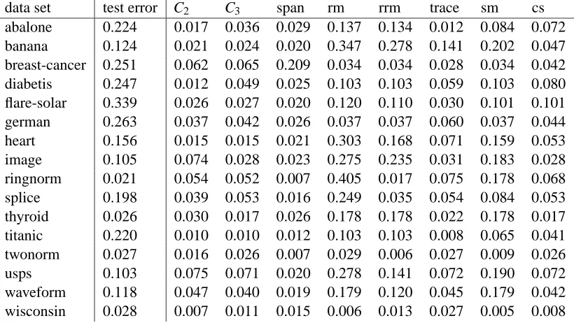
The goal of the next experiment was not only to select the kernel widthσ, but to find the best

values for the kernel widthσ and the soft margin parameter C simultaneously. Its results can be

seen in Table 1, which was produced as follows. For each training set we chose the parameters

σand C for which the respective bounds were minimal, and evaluated the test error for the chosen

parameters. Then we computed the means over the different training runs. The first column contains the mean value of the minimal test error. The other columns contain the offset by which the test errors selected by the different bounds are worse than the optimal test error. On most data sets, the radius margin bound, the rescaled radius margin bound, and the sparse margin bound perform rather poorly. Often their results are worse than those of the other bounds by one order of magnitude.

Among the other bounds, C2and the span bound are the two superior bounds. Between those two

bounds, there is a tendency towards the span bound in this experiment: C2beats the span bound on

6 data sets, the span bound beats C2on 10 data sets. Thus C2does not perform as good as the span

bound, but it gets close.

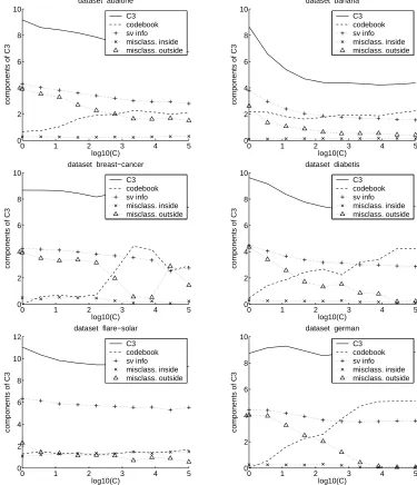
To explain the good performance of the compression coefficients we now want to analyze their properties in more detail. As the compression coefficients are a sum of several terms it is a natural question which of the terms has the largest influence on the actual value of the sum. To answer this

(21)

cor-data set test error C2 C3 span rm rrm trace sm cs

abalone 0.224 0.017 0.036 0.029 0.137 0.134 0.012 0.084 0.072

banana 0.124 0.021 0.024 0.020 0.347 0.278 0.141 0.202 0.047

breast-cancer 0.251 0.062 0.065 0.209 0.034 0.034 0.028 0.034 0.042

diabetis 0.247 0.012 0.049 0.025 0.103 0.103 0.059 0.103 0.080

flare-solar 0.339 0.026 0.027 0.020 0.120 0.110 0.030 0.101 0.101

german 0.263 0.037 0.042 0.026 0.037 0.037 0.060 0.037 0.044

heart 0.156 0.015 0.015 0.021 0.303 0.168 0.071 0.159 0.053

image 0.105 0.074 0.028 0.023 0.275 0.235 0.031 0.183 0.028

ringnorm 0.021 0.054 0.052 0.007 0.405 0.017 0.075 0.178 0.068

splice 0.198 0.039 0.053 0.016 0.249 0.035 0.054 0.084 0.053

thyroid 0.026 0.030 0.017 0.026 0.178 0.178 0.022 0.178 0.017

titanic 0.220 0.010 0.010 0.012 0.103 0.103 0.008 0.065 0.041

twonorm 0.027 0.016 0.026 0.007 0.029 0.006 0.027 0.009 0.026

usps 0.103 0.075 0.071 0.020 0.278 0.141 0.072 0.190 0.072

waveform 0.118 0.047 0.040 0.019 0.179 0.120 0.045 0.179 0.042

wisconsin 0.028 0.007 0.011 0.015 0.006 0.013 0.027 0.005 0.008

Table 1: Model selection results for selecting the kernel widthσand the soft margin parameter C

simultaneously. For each training set and each bound we chose the parametersσand C

(22)

responding to the support vector information, the term log∗n+log n corresponding to the position

of the codebook vector, the term(r+1)log m+r corresponding to the points inside the rotation

re-gion, and the term(l+1)log m corresponding to the information on the misclassified points outside

the rotation region. For each fixed soft margin parameter C we chose the kernel widthσwhere the

value of the compression coefficient C3 is minimal. For this value ofσ, we plotted the means of

the different terms. Here we only show the plots for compression coefficient C3 (as C3 has more

different terms than C2) on the first six data sets (in alphabetical order). The plots on the other data

sets, as well as the plots for C2, are very similar to the ones we show. We find that all terms (except

the term “misclass. inside” which is negligible) are of the same order of magnitude, with no term consistently dominating the other ones. This behavior is attractive as it shows that all different parts of information have substantial influence on the value of the compression coefficient.

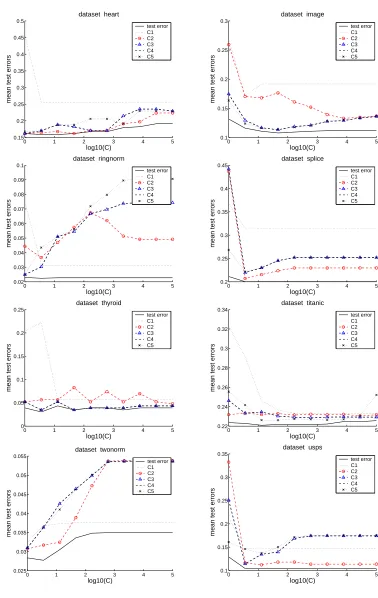
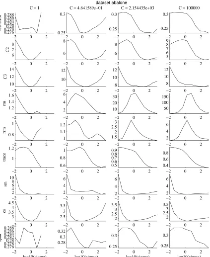
Finally we want to study the shapes of the curves of the different bounds. As we use the values of the bounds to predict the qualitative behavior of the test error it is important that the shapes of the bounds’ curves are similar to the shape of the test error curve. In Figure 6 we plot those shapes for

the compression coefficients C2, C3, and the other bounds versus the kernel widthσ. We show the

plots for every second value of C (to cover the whole range of values of C we used) and for the first six data sets (in alphabetical order). First of all we can observe that the value of the compression coefficient is often larger than 1. This is also the case for several of the other bounds, and is due to the fact that most bounds only yield nontrivial results for very large sample sizes. This need not be a problem for applications as we use the bounds to predict the qualitative behavior of the test error, not the quantitative one. Secondly, the compression scheme and the sparse margin bound suffer from the fact that they only attain finite values when the number of support vectors is smaller than

the number of training vectors. Among all bounds, only C2, C3and the span bound seem to be able

to predict the shape of the test error curve.

The main conclusions we can draw from all experimental results is that in all three tasks

(pre-dicting the shape of the test error curve, choosing parameterσ, choosing parametersσand C) the

span bound and compression coefficient C2 have the best performance among all bounds, where

(23)

0 1 2 3 4 5 0

2 4 6 8 10

dataset abalone

log10(C)

components of C3

C3 codebook sv info misclass. inside misclass. outside

0 1 2 3 4 5

0 2 4 6 8 10

dataset banana

log10(C)

components of C3

0 1 2 3 4 5

0 2 4 6 8 10

log10(C)

components of C3

0 1 2 3 4 5

0 2 4 6 8 10

dataset diabetis

log10(C)

components of C3

0 1 2 3 4 5

0 2 4 6 8 10 12

log10(C)

components of C3

0 1 2 3 4 5

0 2 4 6 8 10

dataset german

log10(C)

components of C3

Figure 5. Here we study the relationship between the different components of C3. We plot the

lengths of the codes for the support vector information (“sv info”), the position of the codebook vector (“codebook”), the information on the points inside the rotation region (“misclass. inside”), and the information about the misclassified points outside the rotation region (“misclass. outside”).

4. Conclusions

(24)

C2because it is easy to compute and yields good results in the experiments. The results it achieves

are comparable to those of the state of the art span bound. The theoretical justification for using compression coefficients are the generalization bounds we cited in Section 2. They were proved in an abstract coding theoretic setting. We now derived methods to apply these bounds in practi-cal applications. This shows that the connection between information theory and learning can be exploited in every-day machine learning applications.

Acknowledgements

(25)

−2 0 2 0.276 0.2780.28 0.282 0.284 0.286 0.288 test error

C = 1

−2 0 2

0.25 0.3

C = 4.641589e+01

−2 0 2

0.25 0.3

C = 2.154435e+03

−2 0 2

0.25 0.3

C = 100000

−2 0 2

6 7 8

C2

−2 0 2

6 8

−2 0 2

6 8

−2 0 2

5 6 7 8 9

−2 0 2

10 12 14

C3

−2 0 2

10 12

−2 0 2

8 10 12

−2 0 2

8 10 12

−2 0 2

1.2 1.4 1.6

rm

−2 0 2

2 4 6

−2 0 2

10 20 30

−2 0 2

50 100 150

−2 0 2

0.8 1

rrm

−2 0 2

1 1.1 1.2

−2 0 2

1.5 2 2.5 3

−2 0 2

2 4 6

−2 0 2

1 1.2

trace

−2 0 2

0.6 0.8 1

−2 0 2

0.5 0.6 0.7 0.8 0.9

−2 0 2

0.4 0.6 0.8

−2 0 2

2 4 6 8 10 sm

−2 0 2

2 4 6

−2 0 2

2 4 6

−2 0 2

2 4 6

−2 0 2

3 3.5 4 4.5

cs

−2 0 2

2.5 3 3.5

−2 0 2

2 2.5 3 3.5

−2 0 2

2 2.5 3 3.5

−2 0 2

0.276 0.2780.28 0.282 0.284 0.286 0.288 span log10(sigma)

−2 0 2

0.28 0.3 0.32

log10(sigma)

−2 0 2

0.25 0.3

log10(sigma)

−2 0 2

0.25 0.3

log10(sigma)

dataset abalone

Figure 6: Shapes of curves. Plotted are the mean values of the bounds themselves over the

differ-ent training runs versus the kernel widthσ, for fixed values of the soft margin parameter

(26)

−2 0 2 0.15 0.2 0.25 0.3 0.35 test error

C = 1

−2 0 2

0.2 0.3 0.4

C = 4.641589e+01

−2 0 2

0.2 0.3 0.4

C = 2.154435e+03

−2 0 2

0.15 0.2 0.25 0.3 0.35

C = 100000

−2 0 2

6 8

C2

−2 0 2

4 6

−2 0 2

4 6 8

−2 0 2

4 6 8

−2 0 2

10 15

C3

−2 0 2

5 10

−2 0 2

5 10

−2 0 2

5 10

−2 0 2

1.4 1.6 1.8

rm

−2 0 2

2 4 6

−2 0 2

5 10 15 20 25

−2 0 2

20 40 60 80 100

−2 0 2

0.8 1 1.2

rrm

−2 0 2

0.8 1 1.2 1.4

−2 0 2

2 4

−2 0 2

2 4 6 8 10 12 14

−2 0 2

1.06 1.08 1.1 1.12 1.14 trace

−2 0 2

0.7 0.8 0.9

−2 0 2

0.6 0.8

−2 0 2

0.5 0.6 0.7 0.8 0.9

−5 0 5

0 10 20

sm

−50 0 5

10 20

−5 0 5

0 10 20

−50 0 5

10 20

−5 0 5

2 4 6

cs

−50 0 5

5

−5 0 5

0 5

−50 0 5

5

−2 0 2

0.15 0.2 0.25 0.3 0.35 span log10(sigma)

−2 0 2

0.2 0.3 0.4

log10(sigma)

−2 0 2

0.2 0.3 0.4

log10(sigma)

−2 0 2

0.2 0.25 0.3 0.35 log10(sigma) dataset banana

(27)

−2 0 2 0.285

0.29 0.295

test error

C = 1

−2 0 2

0.29 0.3 0.31

C = 4.641589e+01

−2 0 2

0.3 0.4

C = 2.154435e+03

−2 0 2

0.3 0.4 0.5

C = 100000

−2 0 2

6 8

C2

−2 0 2

6 8

−2 0 2

6 8 10

−2 0 2

8 10

−2 0 2

10 15

C3

−2 0 2

10 12 14

−2 0 2

10 15

−2 0 2

10 15

−2 0 2

0.5 1 1.5

rm

−2 0 2

2 4 6

−2 0 2

5 10 15 20

−2 0 2

20 40 60

−2 0 2

0.5 1

rrm

−2 0 2

0.8 1 1.2

−2 0 2

1 1.5

−2 0 2

1 2 3

−2 0 2

0.5 1

trace

−2 0 2

0.5 1

−2 0 2

0.5 1

−2 0 2

0.4 0.6 0.81 1.2

−5 0 5

0 2 4

sm

−5 0 5

0 20 40

−5 0 5

0 20 40

−5 0 5

1 2 3

−5 0 5

2 3 4

cs

−5 0 5

2 4 6

−5 0 5

2 4 6

−5 0 5

1.5 2 2.5

−2 0 2

0.28 0.3 0.32

span

log10(sigma)

−2 0 2

0.3 0.32 0.34 0.36 0.38 log10(sigma)

−2 0 2

0.3 0.4 0.5

log10(sigma)

−2 0 2

0.2 0.3

log10(sigma)

(28)

−2 0 2 0.3

0.35

test error

C = 1

−2 0 2

0.3 0.35

C = 4.641589e+01

−2 0 2

0.3 0.35

C = 2.154435e+03

−2 0 2

0.3 0.35

C = 100000

−2 0 2

6 8

C2

−2 0 2

5 6 7

−2 0 2

6 8

−2 0 2

6.57 7.58 8.5

−2 0 2

10 15

C3

−2 0 2

10 12 14

−2 0 2

8 10 12 14

−2 0 2

8 10 12 14

−2 0 2

0.5 1 1.5

rm

−2 0 2

2 4 6

−2 0 2

5 10 15 20 25

−2 0 2

20 40 60 80 100

−2 0 2

0.5 1

rrm

−2 0 2

1 1.2

−2 0 2

1 1.5 2

−2 0 2

2 4

−2 0 2

0.5 1

trace

−2 0 2

0.5 0.6 0.7 0.8 0.9

−2 0 2

0.4 0.6 0.8

−2 0 2

0.4 0.6 0.8

−5 0 5

0 10 20

sm

−50 0 5

10 20

−5 0 5

0 10 20

−50 0 5

10 20

−5 0 5

2 4 6

cs

−50 0 5

5

−5 0 5

0 5

−50 0 5

5

−2 0 2

0.26 0.28 0.3 0.32 0.34 span log10(sigma)

−2 0 2

0.24 0.26 0.280.3 0.32 0.34 log10(sigma)

−2 0 2

0.26 0.28 0.3 0.32 0.34 log10(sigma)

−2 0 2

0.3 0.32 0.34

log10(sigma)

dataset diabetis

(29)

−2 0 2 0.36

0.38 0.4

test error

C = 1

−2 0 2

0.36 0.38 0.4

C = 4.641589e+01

−2 0 2

0.355 0.36 0.365

C = 2.154435e+03

−2 0 2

0.36 0.38

C = 100000

−2 0 2

5 6

C2

−2 0 2

4.5 5 5.5 6 6.5

−2 0 2

4.2 4.4

−2 0 2

4.4 4.6 4.85 5.2 5.4

−2 0 2

12 13

C3

−2 0 2

10 11 12

−2 0 2

9.6 9.810 10.2 10.4 10.6 10.8

−2 0 2

10 10.5 11 11.5

−2 0 2

1.3 1.4 1.5

rm

−2 0 2

2 3 4

−2 0 2

2 4 6 8 10 12

−2 0 2

20 40

−2 0 2

0.82 0.84 0.86 0.880.9 0.92 rrm

−2 0 2

1 1.1 1.2

−2 0 2

1 1.5

−2 0 2

1 2

−2 0 2

1 1.1 1.2

trace

−2 0 2

0.6 0.8 1 1.2

−2 0 2

0.5 1

−2 0 2

0.5 1

−5 0 5

18 20 22

sm

−50 0 5

20 40

−5 0 5

5 10 15

−55 0 5

10 15

−5 0 5

4 6 8

cs

−52 0 5

4 6

−5 0 5

3 4 5

−53 0 5

4 5

−2 0 2

0.36 0.38 0.4

span

log10(sigma)

−2 0 2

0.35 0.4

log10(sigma)

−2 0 2

0.3 0.35

log10(sigma)

−2 0 2

0.25 0.3 0.35

log10(sigma)