Using Local Dependencies within Batches to
Improve Large Margin Classifiers
Volkan Vural [email protected]
Department of Electrical and Computer Engineering Northeastern University
Boston, MA 02115
Glenn Fung [email protected]
Balaji Krishnapuram [email protected] Computer Aided Diagnosis and Therapy
Siemens Medical Solutions Malvern, PA 19355
Jennifer G. Dy [email protected]
Department of Electrical and Computer Engineering Northeastern University
Boston, MA 02115
Bharat Rao [email protected]
Computer Aided Diagnosis and Therapy Siemens Medical Solutions
Malvern, PA 19355
Editor: Lyle Ungar
Abstract
Most classification methods assume that the samples are drawn independently and identically from an unknown data generating distribution, yet this assumption is violated in several real life prob-lems. In order to relax this assumption, we consider the case where batches or groups of samples may have internal correlations, whereas the samples from different batches may be considered to be uncorrelated. This paper introduces three algorithms for classifying all the samples in a batch jointly: one based on a probabilistic formulation, and two based on mathematical programming analysis. Experiments on three real-life computer aided diagnosis (CAD) problems demonstrate that the proposed algorithms are significantly more accurate than a naive support vector machine which ignores the correlations among the samples.
Keywords: batch-wise classification, support vector machine, linear programming, machine
learning, statistical methods, unconstrained optimization
1. Introduction
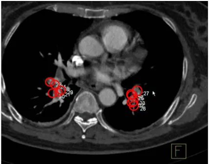
Figure 1: Two pulmonary emboli (blood clots) as they are detected by the Candidate Generation algorithm in a CT image. The candidates are shown as five circles for the left embolus & six circles for the right embolus. The disease status of spatially overlapping or proximate candidates is highly correlated.
is commonly violated in many real-life problems where sub-groups of samples have a high degree of correlation amongst both their features and their labels.
A sample problem with the characteristics described above is computer aided diagnosis (CAD), where the goal is to detect structures of interest to physicians in medical images: for example, to identify potentially malignant tumors in computed tomography (CT) scans, X-ray images, etc. In an almost universal paradigm for CAD algorithms, this problem is addressed by a three-stage system: (1) identification of potentially unhealthy candidates regions of interest (ROI) from a medical image, (2) computation of descriptive features for each candidate, and (3) classification of each candidate (e.g., normal or diseased) based on its features.
Figure 1 displays a CT image of a lung showing circular marks that point to potential diseased candidate regions that are detected by a CAD algorithm. There are five candidates on the left and six candidates on the right (marked by circles) in Figure 1. Descriptive features are extracted for each candidate and each candidate region is classified as normal or abnormal. In this setting, correlations exist among the candidates belonging to the same batch (image, in the case of CAD) both in the training data set and in the unseen testing data. Further, the level of correlation is a function of the pairwise distance between candidates: the disease status (class-label) of a candidate is highly correlated with the status of other spatially proximate candidates, but the correlations decrease as the distance is increased. Most conventional CAD algorithms classify one candidate at a time, ignoring the correlations amongst the candidates in an image. By explicitly accounting for the correlation structure between the labels of the test samples, classification accuracy can be improved.
batch-wise classification to mean training and testing classifiers in batches or groups (i.e., samples
in the same batch are learned and classified collectively). Our experiments on three real CAD prob-lems show that indeed incorporating the local dependencies among samples within a batch improve the classification accuracy significantly compared to standard SVMs.
Beyond the domain of CAD applications, our algorithms are quite general and may be used for batch-wise classification problems in many other contexts. In general, the proposed classifiers can be used whenever data samples are presented in independent batches. In the CAD example, a batch corresponds to an image and strong correlations among candidate samples are based on spatial proximity within an image. A similar relationship structure is true with geographical classification of regions in satellite images; an image would be a batch and spatial proximity corresponds to correlations among the pixel instances. In other contexts, a batch may correspond to data from the same hospital, the patients treated by the same doctor or nurse, etc. In non-medical contexts, a batch can be transactions from the same person, or documents from the same author. Another example is in credit card transaction approval where a single transaction has to be classified by taking into account both the entire set of available training transactions and other transactions made by the same person recently during the testing phase. In this credit card example, it might be preferable to test the recent transaction of this same person as a batch collectively rather than singly.
1.1 Related Work
We are not aware of previous work that exploit internal correlations among the samples to improve the performance of standard classifiers (such as, SVM). However, there exist classification algo-rithms that incorporate special relationships among the samples (the Markov property) into their model formulation. In natural language processing (NLP), conditional random fields (CRF) (Laf-ferty et al., 2001) and recently maximum margin Markov (MMM) networks (Taskar et al., 2004) are used to identify part-of-speech information about words by using the context of nearby words. CRF are also used in similar applications in spoken word recognition. For images, Markov random fields (MRF) (Besag, 1974; Geman and Geman, 1984) are applied to capture correlation among neighborhood pixels.
However, while these Markov models are also fairly general algorithms, they are both compu-tationally demanding and are not easy to implement for problems where the relationship structure among the samples is in any form other than a linear chain (as in the text and speech processing ap-plications). Certainly, their application would be difficult in many large-scale medical applications where run time requirements would be quite severe. For example, in the CAD applications shown in our experiments, the run-time of the testing phase usually has to be less than a second in order that the end user’s (radiologist’s) time would not be wasted.
Our algorithm is also related to the multiple instance learning (MIL) problem, where one is given bags (batches) of samples; class labels are provided only for the bags, not for the individual samples. A bag is labeled positive if we know that at least one sample from it is positive, and a negative bag is known to not contain any positive sample. In this manner, the MIL problem also encodes a form of prior knowledge about correlations between the labels of the training instances.
re-lated to each other, we account for more fine grained differences in the level of correlation between samples (via the similarity matrix R).
Local learning algorithms such as, Wu and Schlkopf (2007) and Bottou and Vapnik (1992), also capture the correlation among data points. However, one major difference between our method and local learning based methods is that our methods build a global classifier that combines the global information extracted from the entire training data with the additional side-information ex-tracted from correlations in the same batch, whereas the local learning algorithms rely on the local information only. Another major difference is that local learning algorithms classify a particular point based on its neighbors in the feature space, therefore the captured correlation is limited to the neighbors of that particular point. On the other hand, the methods that we propose in this paper can incorporate any type of correlation information that is not fully encoded in the features. The same difference is also valid between our method and semi-supervised algorithms such as, Vural et al. (2008) and Zhou et al. (2003) that exploit the idea of using local information in semi-supervised learning. The graph based semi-supervised algorithms such as, Krishnapuram et al. (2005) and Zhu et al. (2003), can be considered to be related to the methods introduced in this paper in the sense that they build weighted graphs based on the correlation among data points. However, the targeted problems in semi-supervised learning and this paper are substantially different. In semi-supervised learning problems, the goal is to make use of unlabeled data to improve classification accuracy. In our methods, on the other hand, we investigate the relations among the data points that are in the same batch only. These data points may not constitute a neighborhood in the feature space and every data point is labeled in our problem.
1.2 Organization of the Paper
After briefly describing the notation in Section 2, we build two SVM based methods for classifying batches of correlated samples in Section 3. We also provide a probabilistic interpretation of our approach in Section 4.
Unlike the previous methods such as CRF, MMM and MRF, the proposed algorithms are easy to implement for arbitrary relationships between samples, and further we are able to run these fast enough to be viable in commercial CAD products. In Section 5, we provide experimental evidence from three different CAD problems to show that the proposed algorithms are more accurate in terms of the metrics appropriate to CAD as compared to a naive SVM which is routinely used for these problems as the state-of-the-art in the current literature and commercial products. We conclude with a review of our contributions in Section 6.
2. Notations
Throughout this paper, we will use the following notations. The capital letters shown in bold font represent matrices whereas lower case letters in bold correspond to vectors. The notation A∈Rm×n will signify a real m×n matrix. For such a matrix, A0 will denote the transpose of A and Ai will denote the i-th row of A. All vectors will be column vectors.
For x∈Rn,kxkpdenotes the p-norm, p=1,2,∞. A vector of ones in a real space of arbitrary dimension will be denoted by e. Thus, for e∈Rmand y∈Rm, e0y is the sum of the components of
y. A vector of zeros in a real space of arbitrary dimension will be denoted by 0. The identity matrix
point sets A and B, is a plane that attempts to separateRninto two half spaces such that each open half space contains points mostly of A or B.
3. A Mathematical Programming Approach
In this section, we formulate the problem of learning for batch-wise prediction as an SVM-like mathematical program.
3.1 Standard Support Vector Machine
In a standard SVM hyperplane classifier, f(x) =x0w−γ is learned from the training instances individually, ignoring the correlations among them. Consider the problem of classifying m points in the n-dimensional real spaceRn, represented by the m×n matrix A, according to class membership
of each point xi(ithrow of A) in the classes A+, A−as specified by a given m×m diagonal matrix
D with +1 or−1 along its diagonal. The standard 1-norm support vector machine with a linear kernel (Vapnik, 1995; Bradley and Mangasarian, 1998) is given by the following linear program with parameterν>0:
min
(w,γ,ξ,v)∈Rn+1+m+nνe
0ξ+e0v (1)
s.t. D(Aw−eγ) +ξ≥e v≥w≥ −v
ξ≥0
where,ξ∈Rm is a vector of slack variables,νis the cost parameter, and at a solution, v=|w|is the absolute value of w. We used the 1-norm linear programming formulation instead of the more popular 2-norm quadratic programming (QP) formulation since the 1-norm formulation is known to produce solutions that depend on fewer features. In other words, by solving the 1-norm formulation, an implicit feature selection is obtained automatically. This is an advantage in CAD applications because the initial pool typically contains a large set of experimental features, although often only a small subset of these features is typically found to be very useful for the classification task at the end of design (i.e., training) stage. It is important to note that all the batch-based classifica-tion approaches presented in this paper are equally applicable even when the standard QP SVM formulation is considered.
3.2 Batch Support Vector Machine
The idea in our model is to encode that the classification of any sample (i.e., data point) depends on two factors: (a) the features that encode information about each candidate sample in a batch; and (b) additional side-information—not already fully encoded in the features—that is available to describe the level of correlations among the set of samples within a batch.1
Let the covariance matrix Rjrepresent the correlations among the samples withing the jthbatch. As mentioned above, in CAD applications, Rjcan be defined in terms of Sj, the matrix of Euclidean distances between candidates inside a medical image (from a patient) as:
Rpqj =
0 ,p=q
exp(−αSpqj ) ,o.w.
with α>0 as a model parameter. Accordingly, Bj∈Rmj×n represents the m
j training points that belong to the jth batch and the labels of these training points are represented by the mj×mj diagonal matrix Dj with positive or negative ones along its diagonal. Using the new notations, the standard SVM set of constraints: D(Aw−eγ) +ξ≥e can be presented as:
Dj(Bjw−eγ) +ξj≥e, for j=1, . . . ,k. (2)
Here, k is defined as the number of batches in A and the vector of slack variables,ξ, in Equation (1) corresponds toξ= [ξ10,ξ20, . . . ,ξk0]0. In Equation (2), every data point in Bj sets a constraint on
w andγindependently, that is, the ith constraint is set by only the ith data point, Bj
i, ignoring the correlations between Bijand the rest of the samples in Bj. Therefore, we modify the standard SVM set of constraints in order to take into account the correlations among samples in the same batches, using the Rj matrix as:
Dj I+θRj(Bjw−eγ)+ξj≥e, for j=1, . . . ,k. (3)
Here,θis a parameter that helps us control the contribution of the correlation information en-coded by Rj. We can find the optimum value ofθby tuning over a validation set. However, we also present a method where we can learnθautomatically in Section 3.3.
In Equation (3), the class membership prediction for any single sample in batch j is a weighted average of the batch members’ prediction vector Bjw−eγ, and the weighting coefficients depend on the pairwise similarity between samples. Using constraints (3) in the SVM formulation (1), we obtain the optimization problem for learning BatchSV M with parametersνandθ:
min
(w,γ,ξ,v)∈Rn+1+m+nνe
0ξ+e0v (4)
s.t. Dj θ
Rj+I
(Bjw−eγ)
+ξj≥e, for j=1, . . . ,k
v≥w≥ −v
ξ≥0.
Whenθ=0, the constraints in Equation (4) become standard SVM constraints. Therefore, if the information provided in Rj matrix does not help our algorithm improve the accuracy performance of SVM, we expect our method to turn into the standard SVM.
Unlike standard SVMs, the hyperplane ( f(x) =w0x−γ) produced by BatchSV M is not the final
decision function. We refer to f(x)as a pre-classifier that will be used in the next stage to make the final decision on a batch of instances. While testing an arbitrary data point xij in batch Bj, the
BatchSV M algorithm accounts for the pre-classifier prediction w0xpj −γ for every member in the batch. The final prediction ˆf(xij)is given by:
sign(fˆ(xj
i)) =sign(w
0
xij−eγ+θRijBjw−eγ). (5)
0 0.2 0.4 0.6 0.8 1 0 0.1 0.2 0.3 0.4 0.5 0.6 0.7 0.8 0.9 1
Positive Data Points Negative Data Points
Batch 1 Batch 2 1 2 3 4 5 6 7 8 9 10
0 0.2 0.4 0.6 0.8 1
0 0.1 0.2 0.3 0.4 0.5 0.6 0.7 0.8 0.9 1
Positive Data Points Negative Data Points
Batch 1 Batch 2 1 2 3 4 5 6 7 8 9 10 a b
0 0.2 0.4 0.6 0.8 1
0 0.1 0.2 0.3 0.4 0.5 0.6 0.7 0.8 0.9 1
Positive Data Points Negative Data Points SVM Batch 1 Batch 2 1 2 3 4 5 6 7 8 9 10
0 0.2 0.4 0.6 0.8 1
0 0.1 0.2 0.3 0.4 0.5 0.6 0.7 0.8 0.9 1
Positive Data Points Negative Data Points BatchSVM Batch 1 Batch 2 1 2 3 4 5 6 7 8 9 10 c d
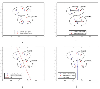
Figure 2: An illustrative example for batch learning. a) Training data points are displayed in batches. b) Relations within training points are displayed as a linked graph. c) Classifier produced by SVM. d) Pre-classifier produced by BatchSV M. Unlike standard SVMs, the hyperplane, f(x), produced by BatchSV M (preclassifier) is not the decision function. Instead, the decision of each test sample xi, is based on a weighted average of the f(x) values for the points linked to xi.
Point Batch Label SVM Pre-classifier Final classifier
1 1 + 0.2826 0.1723 0.1918
2 1 + 0.2621 0.1315 0.2122
3 1 - -0.2398 0.0153 -0.0781
4 1 + -0.3188 -0.0259 0.2909
5 1 - -0.4787 -0.0857 -0.0276
6 2 + 0.2397 0.0659 0.0372
7 2 - 0.2329 0.0432 -0.0888
8 2 + 0.1490 0.0042 0.0680
9 2 - -0.2525 -0.0752 -0.1079 10 2 - -0.2399 -0.1135 -0.1671
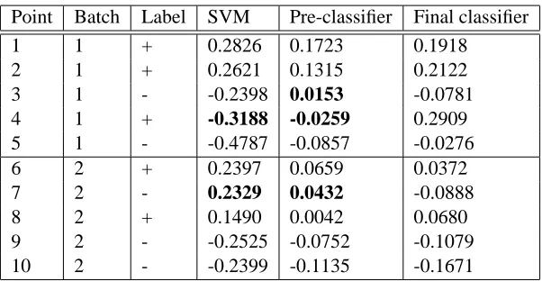
Table 1: Outputs of the classifier produced by SVM, pre-classifier and the final classifier produced by BatchSV M. The outputs are calculated for the data points presented in Figure 2. The first column of the table indicates the order of the data points as they are presented in Figure 2a and the second column specifies the corresponding labels. Misclassified points are displayed in bold. Notice that the combination of the pre-classifier outputs at the final stage corrects the mistakes.
3.3 A Faster Proximal Batch Approach
Support vector machines are known to be slow to train. In Fung and Mangasarian (2001), Fung and Mangasarian introduced proximal support vector machine which is a fast and simple algorithm for generating a linear or nonlinear classifier that merely requires the solution of a single system of linear equations. To yield a faster training method, we present a batch approach to proximal support vector machine in this section.
Similar to the proximal support vector machine formulation (PSVM) in Fung and Mangasarian (2001), we can slightly modify the set of inequalities (3) and consider a Gaussian prior (instead of a Laplacian) for both the error vector ξ and the regularization term, to obtain the following unconstrained formulation:
min
(w,γ)∈Rn+1ν
1 2
k
∑
j=1
ke−Dj θRj+I(Bjw−eγ)k2+1 2(w
0w+γ2). (6)
Note that formulation (6) is a strongly convex (quadratic) unconstrained optimization problem and it has a unique solution. Then, obtaining the solution to formulation (6) requires only solving a single system of linear equations; therefore, it should be substantially faster than the linear pro-gramming approach of the standard QP approach while maintaining approximate accuracy results (Fung and Mangasarian, 2001). Moreover, this simple formulation allows us to introduce a very small modification to learn the parameterθin a very simple but effective manner:
min
(w,γ,θ)∈Rn+1+1ν
1 2
k
∑
j=1
ke−Dj θ
Rj+I
(Bjw−eγ)
k2+1 2(w
This formulation is strongly convex in all its variables (w,γ,θ) and it has a unique solution as well.
The optimization problem (7) can be solved in many different ways, however we chose to use an alternating optimization approach similar to the one used in Fung et al. (2004), since it suits the structure of the problem perfectly and it converged rapidly in our experiments. It took nine iterations on average for the algorithm to converge in our experiments. The alternate optimization method used can be summarized as follows:
0 initialization: Given an initial θ0, the parameter ν, the training data A=Sk
j=1Bj and the corresponding labels D.
1. Solve optimization problem (6) forθ=θi−1obtain wiandγi.
2. For the obtained wiandγi, solve the following linear system of equations:
θi=−∑ k
j=1Mj 2∑kj=1Nj where
Mj =Sj0ZjSj+2e0DjRjSj , for Sj= Bjw−eγ
and Zj= (Rj0+Rj),
Nj =Yj0Yj+1
ν , for Yj=Rj Bjw−eγ
.
This is an iterative method with two steps. At the first step, it finds the optimum values of w andγ(wopt,γopt) for a givenθ. At the second step, for the given woptandγopt, it finds the optimum value ofθ(θopt), which will be used at the first leg of the next iteration. Appendix A.2 provides a derivation of the update equations. Initially, we assign a random value for θ, the procedure is repeated until it converges to the global optimum solution for w,γandθ.
4. A Probabilistic Batch Classification Model
Let xij ∈Rn represent the n features for the ith candidate in the jth image, and let w∈Rn be the weight parameters andγ∈R1be the offset of some hyperplane classifier. Traditionally, classifiers label samples one at a time (i.e., independently) based only on the features that describe a given sample xij:
zij =w0xij−γ = (xij)0w−γ ,zij∈R1.
For example, in logistic regression, the posterior probability of the sample xijbelonging to class +1 is obtained using the sigmoid function P(yij=1|xij) = 1
1+exp(−w0xj
i+γ)
.
For example, in the context of CAD, features describe the shape, size, texture, and intensity profile of a candidate (sample) in an image. However, besides the above information encoded in the form of features that describe each candidate, we also know that correlation amongst the samples in an image (batch) purely based on the proximity of the spatial locations of samples in the jthimage. In CAD applications, this spatial adjacency induces correlations in the predictions for the labels, but in other applications the nature of side-information that accounts for the correlations would be different. Nevertheless, in general (in a domain independent way) we model this side-information as a Gaussian prior on uij.
P(uj∈Rnj) =N(uj|0,Rj) (8)
where nj is the number of the candidates in the jth image, and the covariance matrix Rj encodes the correlations. As mentioned above, in CAD applications, Rj can be defined in terms of S, the matrix of Euclidean distances between candidates inside a medical image (from a patient) as Rj= exp(−αS), withα>0 as a model parameter.
Having defined a prior, next we define the likelihood as follows:
P(zij|uij) =N(zij|uij,σ2). (9) After observing xij and therefore zij, we can modify our prior intuition about ujin (8), based on our observations from (9) to obtain the Bayesian posterior:
P(uj|zj) =N
uj|(Rj−1σ2+I)−1zj;(Rj−1+ 1
σ2I)−1
(10)
The class-membership prediction for the ithcandidate in the jth image is controlled exclusively by
uij. Let Bj∈Rmj×n represent the m
j training points that belong to the jth batch. Exact compu-tation of the integral required for P(yj=1|Bj,w,γ,α,σ2)is analytically infeasible because of the nonlinear sigmoid terms. However, by using the maximum-a-posteriori (MAP) estimate of uij, the prediction probability for class label, yij is then determined approximately as:
P(yij=1|Bj,w,γ,α,σ2)≈1/1+exp−Vj
i[Bjw−eγ]
,
where
Vj=hRj−1σ2+Ii−1.
(11)
Note, however, that for each batch j, the probabilistic method requires calculating two matrix
inversions to computeRj−1σ2+I−1. Hence, training and testing using this method can be time consuming for large batch sizes. On the other hand, Rjθ+I
that we introduced in Equation (3) is relatively less time consuming to compute.
In general,
Rj−1σ2+I
−1
6= Rjθ+I. However, the intuition behind both are similar: the
class prediction for each sample is a weighted sum of the prediction values of the test sample and the samples that are correlated with the test instance. In the appendix A.1, we show that whenσ
is small and we are considering a least squared loss function as in Section 3.3, the constraint (3) results in an approximation to the following constraint:
Dj
Rj−1σ2+I
−1
(Bjw−eγ)
when the sum of the labels of neighboring data points according to each row of Rj is the same or they have similar values. Note that, this is particularly true when Rj only contains information about correlations for a constant number of nearest neighbors for each sample (k-nearest neighbors) and when the assumption that neighboring segments should have similar labels holds.
4.1 Learning in this Model
For batch-wise prediction using (11), w,αandσ2 can be learned from a set of N training images via maximum-a-posteriori (MAP) estimation of w and maximum-likelihood estimation ofα,σ2as follows:
[wˆ,ˆγ,αˆ,σˆ2] =arg max
w,γ,α,σ2P(w)∏Nj=1P(yj|Bj,w,γ,α,σ2)
where, P(yj|Bj,w,γ,α,σ2)is defined as in (11) and P(w)may be assumed to be Gaussian N(w|0,λ). The regularization parameterλis typically chosen by cross-validation. General purpose numerical optimizers such as conjugate gradient algorithms may be used for the above optimization problem.
4.2 Intuition about Batch Classification
Equations (10) and (11) imply thatE[uj|zj] = (Rj−1σ2+I)−1zj. In other words, the class mem-bership prediction for any single sample is a weighted average of the noisy prediction quantity zj (distance to the hyperplane), where the weighting coefficients depend on the pairwise Euclidean distances between samples. Hence, the intuition presented above is that we predict the classes for all the nj candidates in the jthimage together, as a function of the features for all the candidates in the batch (here a batch corresponds to an image from a patient). In every test image, each of the candidates is classified using the features from all the samples in the image. Note that although we classify each instance in a batch at the same time, our algorithm outputs a class for each instance and the class membership for these samples need not be the same.
5. Experiments
In this section, we compare regular SVM, probabilistic batch learning (BatchProb), and BatchSV M. Note that in order to make the comparison consistent, BatchProb was implemented by using the same linear programming formulation as BatchSV M but using Equation (12) instead of Equation (3). We also compare PSVM based techniques introduced in Section 3: (1) the proximal ver-sion of batch learning presented in (6) where θis determined as a parameter via cross-validation (BatchPSV M−cv), and (2) the alternating optimization method presented in (7), whereθis learned automatically (BatchPSV M−learned).
5.1 Implementation Details
We present the details of the similarity function that we used in our experiments and how we tuned the parameters of our methods in the next sections.
5.1.1 THESIMILARITYFUNCTION
the candidates. One needs to produce the Rj matrix using the appropriate similarity metric that represents the pairwise-similarities the best for a particular application.
In our CAD applications, we have used the Euclidean distances between candidates inside a medical image as our similarity metric to define the covariance matrix Rj. Let rpand rqrepresent the coordinates of two candidates, Bpj and Bqj on the jth image. For our experiments, we used the Euclidean distance between rpand rqto define the pairwise-similarity, s(p,q), between Bpj and Bqj as following:
s(p,q) =e− krp−rqk2
ς2 .
If the matrices s(p,q)are sparse, it aids the computational efficiency of our algorithms, both in terms of memory use and speed of implementation. Note also that the matrix is naturally sparse, due to the rapid decrease of the exponential function. Nevertheless, to make the implementation stable and memory efficient (by avoiding storing all the elements of these matrices), we found it useful to discretize the continuous similarity function, s(p,q)to the binary similarity function, s∗(p,q)by applying a threshold as following:
s∗(p,q) =
0 s(p,q)<e−4,
1 s(p,q)≥e−4. (13)
In all experiments, we set the threshold at e−4to provide us with a similarity of one if the neighbor is at a 95% confidence level of belonging to the same density as the candidate assuming that the neighborhood is a Gaussian distribution with mean equal to the candidate and variance ς2= 1α. Each element of the matrix R is given by:
Rpq=s∗(p,q).
In order to observe the effects of binarization of the R matrix, we also run experiments on
BatchSV M without applying the threshold in Equation (13), that is, R=s(p,q). We refer to this version of BatchSV M as BatchSV Mcont in our experiments.
5.1.2 PARAMETERTUNING
All our parameters in these experiments are tuned by 10-fold patient cross-validation on the training data (i.e., the training data is split into ten folds). During cross-validation, a range of parameters (θ,σ,ς)were evaluated for the proposed methods. In BatchPSV M−learned, the parameterθis learned automatically through equation (7).
5.2 Evaluation Method
As we explained earlier, R used in the proposed methods is produced from the spatial locations of the candidates. These spatial locations can be considered as extra information provided to our methods. In order to make fair comparisons between our methods and standard SVM and PSVM, we added the spatial locations (x,y,z coordinates of the candidates in 3D image) to the feature vectors of the candidates.
PE Colon Lung train test train test train test
SVM 16.87 0.00 7.22 0.00 1.58 0.00
BatchProb 19.26 4.71 105.14 18.63 46.42 30.02
BatchSV M 11.39 0.23 13.45 0.91 11.73 2.81
BatchSV Mcont 13.42 0.74 61.09 5.93 14.69 3.01
PSVM 0.22 0.00 0.13 0.00 0.05 0.00
BatchPSV M−cv 1.02 0.23 3.67 0.89 4.80 2.82
BatchPSV M−learned 1.39 0.33 4.08 0.89 5.44 2.79
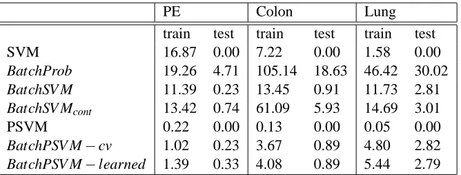
Table 2: Training and testing times for each classifier are displayed in seconds.
lung cancer. In clinical practice, CAD systems are evaluated on the basis of a somewhat domain-specific metric: to maximize the fraction of positives that are correctly identified by the system while displaying at most a clinically acceptable number of false-marks per image. We report this domain-specific metric in an ROC plot, where the y-axis is a measure of sensitivity and the x-axis is the number of false-marks per patient (in our case, per image is also per patient). Sensitivity is the number of patients diagnosed as having the disease divided by the number of patients that has the disease. High sensitivity and low false-marks are desired. All classification algorithms are trained on a training data set and evaluated on a sequestered (held-out) test set.
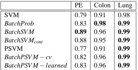
The area under the ROC curve is a commonly used criteria to evaluate the performance of an algorithm. Table 3 displays the area under the ROC curve of each classifier. It is important to note that the areas under the curve presented in Table 3 are calculated considering the entire false positive range which tends to underestimate the superiority of our proposed approach with respect to traditional approaches around the range of false positives acceptable for CAD applications.
PSVM, BatchPSV M−cv and BatchPSV M−learned algorithms require solving a set of linear
equations while training, therefore we expect them to be faster than the other methods mentioned in this paper, namely SVM, BatchProb and BatchSV M. In order to compare the time performances of the methods, we measured the CPU time consumed by each classifier. Table 2, displays the training and testing times required by the algorithms. The training times obtained for the parametric methods (SVM, BatchProb, BatchSV M, PSVM and BatchPSV M−cv) are the total times divided
by the number of cross-validations to find the best value ofθ. On the other hand, the training time for BatchPSV M−learned is the total time divided by the number of iterations that BatchPSV M−
learned required while converging to the optimum value ofθ. We measured the training times this
way to be able to make a fair comparison between the algorithms.
We ran our experiments on an Intel Pentium 4 CPU with 2.8 GHz clock frequency and 1GB RAM and the algorithms were implemented in Matlab.
5.3 Data Sources and Domain Description
0 10 20 30 40 50 60 70 0
0.1 0.2 0.3 0.4 0.5 0.6 0.7 0.8 0.9 1
False positives per patient
Sensitivity
SVM BatchProb BatchSVM BatchSVMcont
10 20 30 40 50 60 70 0.2
0.4 0.6 0.8 1
False positives per patient
Sensitivity
PSVM BatchPSVM−cv BatchPSVM−learned
a b
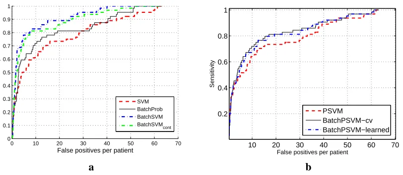
Figure 3: Experimental results for PE data. ROC curves obtained by (a) SVM, BatchProb,
BatchSV M and BatchSV Mcont (b) PSVM, BatchPSV M−cv and BatchPSV M−learned
the pixel intensity descriptive statistics, texture, contrast, 2D and 3D shape descriptors, and the location of the corresponding structure.
5.3.1 EXAMPLE: PULMONARYEMBOLISM
Pulmonary embolism (PE), a potentially life-threatening condition, is a result of underlying venous thromboembolic disease. An early and accurate diagnosis is the key to survival. Computed to-mography angiography (CTA) has emerged as an accurate diagnostic tool for PE. However, there are hundreds of CT slices in each CTA study. Manual reading is laborious, time consuming and complicated by various PE look-alikes (false positives) including respiratory motion artifact, flow-related artifact, streak artifact, partial volume artifact, stair step artifact, lymph nodes, vascular bifurcation among many others (Masutani et al., 2002; Wittram et al., 2004). Several CAD systems are developed to assist radiologists in this process by helping them detect and characterize emboli in an accurate, efficient and reproducible way (Quist et al., 2004; Zhou et al., 2003).
We have collected 72 cases with 242 PEs marked by expert chest radiologists at four different institutions (two North American sites and two European sites). For our experiments, they were randomly divided into two sets: a training and a testing set. The training set was used to train and validate the classifiers and consists of 48 cases with 173 PEs and a total of 3655 candidates. The testing set consists of 24 cases with 69 true PEs out of a total of 1857 candidates. This set was only used to evaluate the performance of the final system. A combined total of 70 features were extracted to describe the shape, texture, size and intensity profile of each candidate.
5.3.2 EXAMPLE: COLONCANCERDETECTION
0 5 10 15 20 25 30 0
0.1 0.2 0.3 0.4 0.5 0.6 0.7 0.8 0.9 1
False Positives per patient
Sensitivity
SVM BatchProb BatchSVM BatchSVM cont
0 5 10 15 20 25 30 0
0.2 0.4 0.6 0.8 1
False positives per patient
Sensitivity
PSVM BatchPSVM−cv BatchPSVM−learned
a b
Figure 4: Experimental results for Colon Cancer data. ROC curves obtained by (a) SVM, BatchProb, BatchSV M and BatchSV Mcont (b) PSVM, BatchPSV M−cv and
BatchPSV M−learned
cancer progressed rapidly is from local (polyp adenomas) to advanced stages (colorectal cancer), which has very poor survival rates. However, identifying (and removing) lesions (polyp) when still in a local stage of the disease, has very high survival rates, thus illustrating the critical need for early diagnosis. The sizes of a polyp in the colon can vary from 1mm all the way up to 10cm. Most polyps no matter how small they are, are represented by two candidates; one obtained from the prone view and the other one from the supine view. Moreover, for large polyps or so called masses a typical candidate generation algorithm generates several candidates across the polyp surface. Therefore most polyps in the training data are inherently represented by multiple candidates.
For the sake of clinical acceptability, it is sufficient to detect one of these candidates during classification. Unlike a standard classification algorithm where the emphasis is to accurately classify each and every candidate, here we seek to classify at least one of the candidates representing a polyp accurately. The database of high-resolution CT images used in this study were obtained from seven different sites across US, Europe and Asia. The 188 patients were randomly partitioned into a training and a test set. The training set consists of 65 cases containing 127 volumes. Fifty polyps were identified in this set out of a total of 6748 candidates. The testing set consists of 123 cases containing 237 volumes. There are 103 polyps in this set from a total of 12984 candidates. A total of 75 features were extracted to describe the shape, size, texture and intensity profile of each candidate.
5.3.3 EXAMPLE: LUNGCANCER
2 4 6 8 10 12 14 16 18 0.55
0.6 0.65 0.7 0.75 0.8 0.85 0.9 0.95
False positives per patient
Sensitivity
SVM BatchProb BatchSVM BatchSVM cont
0 2 4 6 8 10 12 14 16 18
0.1 0.2 0.3 0.4 0.5 0.6 0.7 0.8 0.9
False positive per patient
sensitivity
PSVM BatchPSVM−cv BatchPSVM−learned
a b
Figure 5: Experimental results for Lung Cancer data. ROC curves obtained by (a) SVM, BatchProb, BatchSV M and BatchSV Mcont (b) PSVM, BatchPSV M−cv and
BatchPSV M−learned
and only a few (≤5 on average) of which are potential nodules that should be identified as positive by LungCAD, all within the run-time requirements of completing the classification on-line during the time the physician completes their manual review.
The training set consists of 60 patients. The number of candidates labeled as nodules in the train-ing set are 157 and the total number of candidates is 9987. The testtrain-ing set consists of 26 patients. In this testing set, there are 79 candidates labeled as nodules out of 6159 generated candidates. A total of 15 features were used to describe the shape, size, texture and intensity profile of each candidate region.
5.4 Discussion and Results
In our experiments, we would like to find out whether the batch methods are better than the stan-dard SVM, whether BatchSV M is better than BatchProb in terms of accuracy and speed, whether BatchPSV M is as accurate as BatchSV M, whether BatchPSV M is faster than BatchSV M, and whether the automated tuning works by comparing BatchPSV M−learned with BatchPSV M−cv.
5.4.1 SVMVERSUSBATCHMETHODS
Figures 3, 4, and 5 show the ROC curves for pulmonary embolism, colon cancer, and lung cancer data respectively. In our medical applications high-sensitivity is critical as early detection of lung and colon cancer is believed to greatly improve the chances of successful treatment (Bogoni et al., 2005). Furthermore, high specificity is also critical, as a large number of false positives will vastly increase physician load and lead (ultimately) to loss of physician confidence.
PE Colon Lung
SVM 0.79 0.91 0.98
BatchProb 0.83 0.98 0.99
BatchSV M 0.89 0.96 0.99
BatchSV Mcont 0.88 0.95 0.99
PSVM 0.77 0.91 0.99
BatchPSV M−cv 0.82 0.96 0.99 BatchPSV M−learned 0.83 0.96 0.99
Table 3: Area under the ROC curves for each classifier. (Best in bold).
64% sensitivity. As seen from the figure, the two proposed methods are substantially more accurate than standard SVMs at any specificity level. When we compare the performances of PSVM and
BatchPSV M−learned in Figure 3b, we observe that the proposed batch method (BatchPSV M−
learned) dominates over PSVM. However, they do not improve the accuracy of PSVM as much as BatchProb and BatchSV M do.
Colon cancer data is a relatively easier data set than pulmonary embolism since standard SVM can achieve 54.5% sensitivity at one false positive level as illustrated in Figure 4a. However,
BatchSV M improved SVM’s performance to 84% sensitivity for the same number of false
posi-tives. Note that BatchProb improved the sensitivity further, giving 89.6% for the same specifity. In one to ten false positives region which constitutes the region of interest in our applications, our proposed methods outperform standard SVM significantly. PSVM’s performance is substantially worse than that of our proposed batch methods, BatchPSV M−cv and BatchPSV M−learned.
Although SVM is very accurate for the lung cancer application, Figure 5a shows that BatchProb and BatchSV M could still improve SVM’s performance further. BatchProb method is superior to the other methods at two and three false positives per image. Both BatchProb and BatchSV M outperform SVM in the 2-6 false positives per image region, which is the region of interest for commercial clinical lung CAD systems. All three of the methods are comparable at other specificity levels. On the other hand, we observe in Figure 5b that BatchPSV M−cv and BatchPSV M−learned
methods did not achieve significant improvements, yet they are still comparable to PSVM.
When we consider the area under the ROC curve for each of the methods in Table 3, we observe that our proposed methods are better than SVM and PSVM in every case except one where PSVM performs the same as our proposed methods in the lung cancer data.
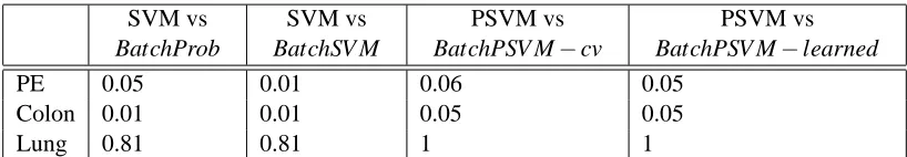
SVM vs
BatchProb
SVM vs
BatchSV M
PSVM vs
BatchPSV M−cv
PSVM vs
BatchPSV M−learned
PE 0.05 0.01 0.06 0.05
Colon 0.01 0.01 0.05 0.05
Lung 0.81 0.81 1 1
Table 4: P-values that indicate the confidence level of significance when the proposed algorithms are compared to SVM and PSVM in terms of the area under the ROC curves.
5.4.2 BatchSV M VERSUSBatchProb
As we discussed in Section 3, BatchProb requires calculating two matrix inversions, which can be time consuming for large sizes of batches, whereas BatchSV M avoids matrix inversions, therefore
BatchSV M should be faster than BatchProb in both training and testing. As expected, our
experi-ments show us that BatchSV M is faster than BatchProb in every case. Note that the difference in run times is significant for testing in PE and Colon data sets, where BatchSV M is twenty times faster than BatchProb. On the other hand, BatchProb produced a better ROC curve in Colon data set. Therefore, although BatchProb is slow compared to BatchSV M, it may be preferable with respect to accuracy depending on the application.
5.4.3 BatchPSV M−learnedVERSUSBatchPSV M−cv
BatchPSV M−cv requires cross-validated tuning over the parameterθto achieve the optimum accu-racy. One problem with tuning is that we can only tune the parameter in a limited range. Therefore a good guess of the range of the parameter values is crucial. Another problem is that we can only tune the parameter over discrete values which may not include the best parameter value. One way to obtain a close approximation of the best parameter value is to divide the range of the parameter into small steps. However this method will increase the training time since cross-validation will be repeated as many times as the possible parameter values (in our experiments, we cross-validated θover 21 values). On the other hand, automated tuning (BatchPSV M−learned) is quite feasible
and avoids the problems stated above. In our experiments, BatchPSV M−learned was able to
au-tomatically converge to the optimum value ofθin only nine iterations on average while producing comparable ROC plots with cross-validated tuning (BatchPSV M−cv) as seen in Figures 3b, 4b and
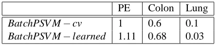
5b. The optimumθvalues obtained by cross-validated tuning and automated tuning are presented in Table 5. As observed in the table, the optimumθvalues found by both algorithms are very similar.
When we compare the two methods with respect to training times, we observe that BatchPSV M−
cv is faster than BatchPSV M−learned for a fixed value ofθ. However, since we repeated
cross-validation 21 times for BatchPSV M−cv and BatchPSV M−learned required nine iterations on
average, BatchPSV M−learned is actually faster than BatchPSV M−cv in overall while training.
5.4.4 BatchPSV M VERSUSBatchSV M
BatchSV M results in a linear programming problem, whereas BatchPSV M requires solving a set
PE Colon Lung
BatchPSV M−cv 1 0.6 0.1
BatchPSV M−learned 1.11 0.68 0.03
Table 5:θvalues obtained by BatchPSV M−cv and BatchPSV M−learned.
BatchPSV M in the training phase. However, despite the training time performance, BatchSV M
produced better ROC curves than that of BatchPSV M in PE and lung cancer data sets as illustrated in Figures 3 and 5 respectively. The area under the ROC curve produced by BatchSV M is also better than BatchPSV M for these two data sets. For Colon data set, in Figure 4b, we observe that
BatchPSV M−cv and BatchSV M performed slightly better than BatchSV M−learned where both
achieve 86% sensitivity at one false positive level. Furthermore, the total area under the ROC curves produced by BatchSV M and BatchPSV M are the same (0.96). From the experimental results, we can draw the conclusion that BatchPSV M is a fast alternative to BatchSV M and can be preferable in some applications.
6. Conclusions
Three related algorithms have been proposed for classifying batches of correlated data samples. Al-though primarily motivated by real-life CAD applications, the problem occurs commonly in many situations; our algorithms are sufficiently general to be applied in other contexts. Experimental re-sults indicate that the proposed method can substantially improve the diagnosis of (a) early stage cancer in the Lung & Colon, and (b) pulmonary embolisms (which may result in strokes). With the increasing adoption of these systems in routine clinical practice, these experimental results demon-strate the potential of our methods to impact a large cross-section of the population.
In this paper, we validated the improvement in diagnosis sensitivity that batch-wise classifica-tion provides to CAD problems. The algorithms presented here are general and can be applied to other domains. In other domains, one may apply other similarity metric appropriate for the appli-cation. For data with no clear batch information, clustering can be performed to create the batches. Extending the batch algorithms to other data and automatically learning the similarity metric are topics for future work.
Acknowledgments
This research is supported by Siemens Medical Solutions USA, Inc. and NSF CAREER IIS-0347532.
Appendix A.
A.1 Connection between Equations (3) and (12)
We will show the connection between the optimization problems that result by considering the constraints (3) and (12) by proving that the resulting objective functions are closely related to each other.
First, let us show that the inverse
I+Rj−1σ2
−1
that appears in Equation (12) can be
approx-imated by the expression I−σ2Rj−1.
By replacing A=σ2Rj−1, in the identity:
(I+A)−1=I−A+A2−A3+. . .+,∀A
we have:
I+Rj−1σ2
−1
=I−σ2Rj−1+σ4Rj−1Rj−1−. . .
where the termsσ4Rj−1Rj−1−σ6Rj−1Rj−1Rj−1+. . .can be ignored ifσis sufficiently small. Then, we have:
I+Rj−1σ2
−1
∼
= I−σ2Rj−1
= −σ2Rj−1 I+θRj (14)
whereθ=−1
σ2 provided thatσ6=0.
Let us recall that the quadratic unconstrained objective function that results from the constraint (12) is:
min
(w,γ,θ)∈Rn+1+1ν
1 2
k
∑
j=1
e−Dj
σ2Rj−1+I−1(Bjw−eγ)
2 +1
2(w
0w+γ2+θ2) (15)
and that the quadratic unconstrained objective function that results from the constraint (3) is given by:
min
(w,γ,θ)∈Rn+1+1ν
1 2
k
∑
j=1
e−Dj
θ
Rj+I
(Bjw−eγ)
2 +1
2(w
0w+γ2+θ2). (16)
Next, we will show that the objective functions (15) and (16) are related to each other under certain assumptions. In order to ease the notation, let’s now define
g(w,γ) =
k
∑
j=1
e−Dj
σ2Rj−1+I−1(Bjw−eγ)
2 .
Then ifσ2is small we have from (14) that:
g(w,γ) ≈ ∑k j=1
e−D
jh−σ2Rj−1 θRj+I
(Bjw−eγ)
i
2 = ∑kj=1
−σ2Rj−1 −1
σ2Rj
e−Dj θRj+I(Bjw−eγ)
2 ≤ ∑kj=1
σ
2Rj−1
2
−σ12Rj
e−Dj θRj+I(Bjw−eγ)
2 ≤ Ψ∑k
j=1
−σ12Rje−Dj
θ
Rj+I
(Bjw−eγ)
2
whereΨ=maxj{
σ
2Rj−1
2
}, then, ifσis small we can conclude that f(w,γ) is approximately a “good” upper bound for g(w,γ). Furthermore if h(w,γ,θ) =w0w+γ2+θ2,then F(w,γ,θ) = ν1
2f(w,γ) + 1
2h(w,γ,θ)is also a “good” upper bound for G(w,γ,θ) =ν 1
2g(w,γ) + 1
2h(w,γ,θ). So intuitively, since G(w,γ,θ)and F(w,γ,θ)are non-negative convex quadratic functions, mini-mizing F(w,γ,θ)should provide good approximate solutions to the problem of minimizing G(w,γ,θ).
Let us assume now that the number of neighboring points that affect the classification for every point is more or less constant. This is true when R is binary and calculated only for the k nearest neighbors or when the rows of R are normalized and approximately true when R is defined as in (13). This is equivalent to assuming that the summation of all the rows of R is constant, or equivalently, for every batch j:
−1 σ2R
je≈ke
where k is a constant. hence:
f(w,γ) =
k
∑
j=1
ke−Dj
θ
Rj+I(Bjw−eγ)
2
.
Then, solving the problem:
minw,γ,θF(w,γ,θ)
is equivalent to solving the proximal batch formulation presented in Equation (7) for someν=ν¯ (the constant k only rescales the problem in the variables w andγ).
A.2 Derivation for Automatically Tuning the Parameters in BatchPSVM
The optimization problem in (7) is a bi-convex problem and can be solved in an iterative fashion with two steps. At the first step, we find the optimum values of w andγ(wopt,γopt) for a givenθ. At the second step, for wopt andγopt held fixed, we find the optimum value ofθ(θopt), which will be used at the first leg of the next iteration.
A.2.1 OPTIMIZING FORwANDγWITHθFIXED
Given θ is held fixed, we can optimize (7) with respect to w andγ, and rewrite the equation as follows:
min
(w,γ)∈Rn+1
1 2µ
k
∑
j=1
x0Pjx+qjx+K1, where x= w γ ,
Pj=
1
µI+θ2Bj
0
Rj0RjBj+θBj0(Rj0+Rj)Bj+Bj0Bj −θ2Bj0Rj0Rje−θBj0(Rj0+Rj)e−Bj0e
−θ2e0Rj0RjBj−θe0(Rj0+Rj)Bj−e0Bj θ2e0Rj0Rje+θe0(Rj0+Rj)e+e0e+1 µ
,
qj=2
−θe0DjRjBj−e0DjBj
−θe0DjRje+e0Dje
and K1is a constant term with respect to w andγ.
After taking the derivative of the objective function with respect to x and equating to zero, we can obtain the solution as following:
x=−( k
∑
j=1
Pj)−1( k
∑
j=1
qj)
A.2.2 OPTIMIZING FORθWITHwANDγFIXED
When w andγhave fixed values, we can rewrite Equation (7) consideringθis the only variable as following:
min
(w,γ)∈Rn+1
1 2µ
k
∑
j=1
θ2Nj+θMj+K 2 where K2is a constant with respect toθand
Nj= w0Bj0Rj0RjBjw−w0Bj0Rj0Rjeγ−γe0Rj0RjBjw+γ2e0Rj0Rje+1 µ
and
Mj= −e0DjRjBjw+e0DjRjeγ−w0Bj0Rj0Dj0e+w0Bj0Rj0Bjw−w0Bj0Rj0eγ
+γe0Rj0Dj0e−γe0Rj0Bjw+γe0Rj0eγ+w0Bj0RjBjw−w0Bj0Rjeγ
−γe0RjBjw+γe0Rje
.
Mj can be further simplified as:
Mj= w0Bj0(Rj0+Rj)Bjw−w0Bj0(Rj0+Rj)eγ−γe0(Rj0+Rj)Bjw
+γe0(Rj0+Rj)eγ−2e0DjRjBjw+2e0DjRjeγ
using the property that A0=A, if A is a scalar.
References
J. Besag. Spatial interaction and the statistical analysis of lattice systems. Journal of the Royal
Statistical Society, Series B, 36:192–236, 1974.
L. Bogoni, P. Cathier, M. Dundar, A. Jerebko, S. Lakare, J. Liang, S. Periaswamy, M. Baker, and M. Macari. CAD for colonography: A tool to address a growing need. British Journal of
Radiol-ogy, 78:57–62, 2005.
L. Bottou and V.N. Vapnik. Local learning algorithms. Neural Computation, 4(6):888–900, 1992.
URLciteseer.ist.psu.edu/bottou92local.html.
G. Fung and O. L. Mangasarian. Proximal support vector machine classifiers. In Knowledge
Dis-covery and Data Mining, pages 77–86, 2001.
G. Fung, M. Dundar, J. Bi, and B. Rao. A fast iterative algorithm for fisher discriminant using heterogeneous kernels. In ICML ’04: Proceedings of the twenty-first international conference on
Machine learning, page 40, New York, NY, USA, 2004. ACM Press. ISBN 1-58113-828-5. doi:
http://doi.acm.org/10.1145/1015330.1015409.
S. Geman and D. Geman. Stochastic relaxation, Gibbs distribution and the Bayesian restoration of images. IEEE Transactions on Pattern Analysis and Machine Intelligence, 6(6):721–741, 1984.
J.A. Hanley and B.J. McNeil. A method of comparing the areas under receiver operating char-acteristic curves derived from the same cases. Radiology, 148(3):839–843, 1983. URL
http://radiology.rsnajnls.org/cgi/content/abstract/148/3/839.
D. Jemal, R. Tiwari, T. Murray, A. Ghafoor, A. Samuels, E. Ward, E. Feuer, and M. Thun. Cancer statistics. CA Cancer J. Clin., 54:8–29, 2004.
B. Krishnapuram, D. Williams, Y. Xue, A. Hartemink, L. Carin, and M. Figueiredo. On semi-supervised classification. In NIPS 17, pages 721–728. MIT Press, 2005.
J. Lafferty, A. McCallum, and F. Pereira. Conditional random fields: Probabilistic models for segmenting and labeling sequence data. In Proc. 18th International Conf. on Machine Learning, pages 282–289, San Francisco, CA, 2001. Morgan Kaufmann.
Y. Masutani, H. MacMahon, and K. Doi. Computerized detection of pulmonary embolism in spiral CT angiography based on volumetric image analysis. IEEE Transactions on Medical Imaging, 21:1517–1523, 2002.
M. Quist, H. Bouma, C. Van Kuijk, O. Van Delden, and F. Gerritsen. Computer aided detection of pulmonary embolism on multi-detector CT. In Proceedings of the 90th Meeting of the
Radiolog-ical Society of North America (RSNA), 2004.
B. Taskar, C. Guestrin, and D. Koller. Max-margin Markov networks. In Sebastian Thrun, Lawrence Saul, and Bernhard Sch ¨olkopf, editors, Advances in Neural Information Processing Systems 16. MIT Press, Cambridge, MA, 2004.
V. N. Vapnik. The Nature of Statistical Learning Theory. Springer, New York, 1995.
V. Vural, G. Fung, J. Dy, and Rao B. Fast semi-supervised svm classifiers using a-priori metric information. Optimization Methods and Software (OMS), 23(4):521–532, 2008.
C. Wittram, M. Maher, A. Yoo, M. Kalra, O. Jo-Anne, M. Shepard, and T. McLoud. CT angiography of pulmonary embolism: Diagnostic criteria and causes of misdiagnosis. RadioGraphics, 24: 1219–1238, 2004.
M. Wu and B. Schlkopf. Transductive classification via local learning regularization. In 11th
International Conference on Artificial Intelligence and Statistics, pages 628–635, Brookline, MA,
C. Zhou, L. M. Hadjiiski, B. Sahiner, H.-P. Chan, S. Patel, P. Cascade, E. A. Kazerooni, and J. Wei. Computerized detection of pulmonary embolism in 3D computed tomographic (CT) images: ves-sel tracking and segmentation techniques. In Medical Imaging 2003: Image Processing. Edited
by Sonka, Milan; Fitzpatrick, J. Michael. Proceedings of the SPIE, Volume 5032, pp. 1613-1620 (2003)., pages 1613–1620, May 2003. doi: 10.1117/12.481369.
D. Zhou, O. Bousquet, T. Navin Lal, Jason Weston, and Bernhard Sch ¨olkopf. Learning with local and global consistency. In Advances in Neural Information Processing Systems. MIT Press, 2003.