A New Approach to Collaborative Filtering: Operator Estimation with Spectral Regularization

(1)

A New Approach to Collaborative Filtering:

Operator Estimation with Spectral Regularization

Division of Computer Science University of California

387 Soda Hall, Berkeley, CA, USA

INRIA - WILLOW Project-Team

Laboratoire d’Informatique de l’Ecole Normale Sup´erieure (CNRS/ENS/INRIA UMR 8548) 45, rue d’Ulm, 75230 Paris, France

Theodoros Evgeniou [email protected]

Decision Sciences and Technology Management INSEAD

Bd de Constance, 77300 Fontainebleau, France

Jean-Philippe Vert∗ [email protected] Mines ParisTech

Centre for Computational Biology

35 rue Saint-Honor´e, 77300 Fontainebleau, France

Editor: Tommi Jaakkola

Abstract

We present a general approach for collaborative filtering (CF) using spectral regularization to learn linear operators mapping a set of “users” to a set of possibly desired “objects”. In particular, sev-eral recent low-rank type matrix-completion methods for CF are shown to be special cases of our proposed framework. Unlike existing regularization-based CF, our approach can be used to incor-porate additional information such as attributes of the users/objects—a feature currently lacking in existing regularization-based CF approaches—using popular and well-known kernel methods. We provide novel representer theorems that we use to develop new estimation methods. We then provide learning algorithms based on low-rank decompositions and test them on a standard CF data set. The experiments indicate the advantages of generalizing the existing regularization-based CF methods to incorporate related information about users and objects. Finally, we show that certain multi-task learning methods can be also seen as special cases of our proposed approach.

Keywords: collaborative filtering, matrix completion, kernel methods, spectral regularization

1. Introduction

Collaborative filtering (CF) refers to the task of predicting preferences of a given “user” for some “objects” (e.g., books, music, products, people, etc.) based on his/her previously revealed preferences—typically in the form of purchases or ratings—as well as the revealed preferences of other users. In a book recommender system, for example, one might like to suggest new books

(2)

to a new user based on what she and other users have recently purchased or rated. The ultimate goal of CF is to infer the preferences of users in order to offer them new objects.

A number of CF methods have been developed in the past (Breese et al., 1998; Heckerman et al., 2000; Salakhutdinov et al., 2007). Recently there has been interest in CF using regularization-based methods (Srebro and Jaakkola, 2003). This work adds to that literature by developing a novel general approach to regularization-based CF methods.

Recent regularization-based CF methods assume that the only data available are the revealed preferences, where no other information such as background information on the objects or users is given. In this case, one may formulate the problem as that of inferring the contents of a partially observed preference matrix: each row represents a user, each column represents an object (e.g., books or movies), and entries in the matrix represent a given user’s rating of a given object. When the only information available is a set of observed user/object ratings, the unknown entries in the matrix must be inferred from the known ones—of which there are typically very few relative to the size of the matrix.

To make useful predictions within this setting, regularization-based CF methods make certain assumptions about the relatedness of the objects and users. The most common assumption is that the preference function can be decomposed into a small number of factors, resulting in the search for a low-rank matrix which approximates the partially observed matrix of preferences (Srebro and Jaakkola, 2003). The rank constraint can be interpreted as a regularization on the hypothesis space. Since the rank constraint gives rise to a non-convex set of matrices, the associated optimization problem will be a difficult non-convex problem for which only heuristic algorithms exist (Srebro and Jaakkola, 2003). An alternative formulation, proposed by Srebro et al. (2005), suggests penalizing the predicted matrix by its trace norm, that is, the sum of its singular values. An added benefit of the trace norm regularization is that, with a sufficiently large regularization parameter, the final solution will be low-rank (Fazel et al., 2001; Bach, 2008).

However, a key limitation of current regularization-based CF methods is that they do not take advantage of additional information, such as known attributes of each user (e.g., gender, age) and object (e.g., book’s author, genre), which is often available. Intuitively, such information might be useful to guide the inference of preferences, in particular for users and objects with very few known ratings. For example, at the extreme, users and objects with no prior ratings can not be considered in the standard CF formulation, while their attributes alone could provide some basic preference inference.

(3)

an empirical loss penalized by the norm in a Reproducing Kernel Hilbert Space (RKHS) to more general penalty functions and function classes.

We also show that, with the appropriate choice of kernels for both users and objects, we may consider a number of existing machine learning methods as special cases of our general framework. In particular, we show that several CF methods such as rank-constrained optimization, trace-norm regularization, and those based on Frobenius norm regularization, can all be cast as special cases of spectral regularization on operator spaces. Moreover, particular choices of kernels lead to specific sub-cases such as regular matrix completion and multi-task learning. In the specific application of collaborative filtering with the presence of attributes, we show that our generalization of these sub-cases leads to better predictive performance.

The outline of the paper is as follows. In Section 2, we review the notion of a compact op-erator on Hilbert Space, and we show how to cast the collaborative filtering problem within this framework. We then introduce spectral regularization and discuss how rank constraint, trace norm regularization, and Frobenius norm regularization are all special cases of spectral regularization. In Section 3, we show how our general framework encompasses many existing methods with proper choice of the loss function, the kernels, and the spectral regularizer. In Section 4, we provide three representer theorems for operator estimation with spectral regularization that allow for efficient learning algorithms. Finally in Section 5 we present a number of algorithms and describe several techniques to improve efficiency. We test these algorithms in Section 6 on synthetic examples and a widely used movie database.

2. Learning Compact Operators with Spectral Regularization

In this section we propose a mathematical formulation for a general CF problem with spectral regularization. We then show in Section 3 how several learning problems can be cast under this general framework.

2.1 A General CF Formulation

We consider a general CF problem in which our goal is to model the preference of a user described by x for an item described by y. We denote by x and y the data objects containing all relevant or available information; this could, for example, include a unique identifier i for the i-th user or object. Of course, the users and objects may additionally be characterized by known attributes, in which case x or y might contain some representation of this extra information. Ultimately, we would like to consider such attribute information as encoded in some positive definite kernel between users, or equivalently between objects. This naturally leads us to model the users as elements in a Hilbert space

X

, and the objects they rate as elements of another Hilbert space

Y

.

, with respective dimensions mX and mY.

to

Y

. For an introduction to relevant concepts in functional analysis, see Appendix A.

In the general case we consider below, if

X

and

Y

are not Hilbert spaces, one could also first map (implicitly) users x and objects y into possibly infinite dimensional Hilbert feature spaces ΦX(x)

andΨY(y)and use kernels. We refer the reader to Appendix A for basic definitions and properties

related to compact operators that are useful below. The inference problem can now be stated as follows:

Given a training set of ratings, how may we estimate a “good” compact operator F to predict future ratings?

We estimate the operator F in (1) from the training data using a standard regularization and statistical machine learning approach. In particular, we propose to define the operator as the solution of an optimization problem over

B0

(

Y

,

X

) whose objective function balances a data fitting term RN(F), which is small for operators that can correctly explain the training data, with a regularization

termΩ(F)that controls the complexity of the desired operator. We now describe these two terms in more details.

2.2 Data Fitting Term

Given a loss functionℓ(t′,t)that quantifies how good a prediction t′∈R_{is if the true value is t}_∈R_,

we consider a fitting term equal to the empirical risk, that is, the mean loss incurred on the training set:

RN(F) =

1 N

N

∑

i=1

ℓ(hxi,Fyii_X,ti). (2)

The particular choice of the loss function should typically depend on the precise problem to be solved and on the nature of the variables t to be predicted. See more details in Section 3. In particular, while the representer theorems presented in Section 4 do not need any convexity with respect to this choice, the algorithms presented in Section 5 do.

2.3 Regularization Term

For the regularization term, we focus on a class of spectral functions defined as follows.

Definition 1 A functionΩ:

B0

(

Y

,

X

)7→R_{∪ {}₊∞_}_{is called a spectral penalty function if it can be}

written as:

Ω(F) =

d

∑

i=1

si(σi(F)), (3)

where for any i≥1,si:R+7→R+∪ {+∞}is a non-decreasing penalty function satisfying s(0) =0,

(5)

Note that, by the spectral theorem presented in Appendix A, any compact operator can be decom-posed into singular vectors, with singular values being a sequence that tends to zero.

Spectral penalty functions include as special cases several functions often encountered in matrix completion problems:

• For a given integer r, consider taking si =0 for i=1, . . . ,r, sr+1(u) =0 for u=0, and sr+1(u) = +∞when u>0. This leads to the function:

Ω(F) =

(

0 if rank(F)≤r,

+∞ otherwise. (4)

In other words, the set of operators F that satisfyΩ(F)<+∞is the set of operators with rank smaller than r.

• Taking si(u) =u for all i results in the trace norm penalty (see Appendix A):

Ω(F) =

(

kFk1 if F∈

B1

(

Y

,

X

),

+∞ otherwise, (5)

where we note with

B1

(

Y

,

X

)the set of operators with finite trace norm. Such operators are referred to as trace class operators.

• Taking si(u) =u2 for all i results in the squared Hilbert-Schmidt norm penalty (also called

squared Frobenius norm for matrices, see Appendix A):

Ω(F) =

( kFk2

2 if F∈

B2

(

Y

,

X

),

+∞ otherwise, (6)

where we note with

B2

(

Y

,

X

)the set of operators with finite squared Hilbert-Schmidt norm. Such operators are referred to as Hilbert Schmidt operators.

These particular functions can be combined together in different ways. For example, we may constrain the rank to be smaller than r while penalizing the trace norm of the matrix, which can be obtained by setting si(u) =u for i=1, . . . ,r and sr+1(u) = +∞if u>0. Alternatively, if we want to penalize the Frobenius norm while constraining the rank, we set si(u) =u2 for i=1, . . . ,r

and sr+1(u) = +∞if u>0. We state these two choices of Ωexplicitly since we use these in the experiments (see Section 6) or to design efficient algorithms (see Section 5):

Trace+Rank Penalty: Ω(F) =

(

kFk1 if rank(F)≤r,

+∞ otherwise. (7)

Frobenius+Rank Penalty: Ω(F) =

( kFk2

(6)

2.4 Operator Inference

With both a fitting term and a regularization term, we can now formally define our inference ap-proach. It consists of finding an operator ˆF, if there exists one, that solves the following optimization problem:

ˆ

F∈ arg min

F∈B0(Y,X)

RN(F) +λΩ(F), (8)

whereλ∈R₊_{is a parameter that controls the trade-off between fitting and regularization, and where}

RN(F) and Ω(F) are respectively defined in (2) and (3). We note that if the set {F∈

B0

(

Y

,

X

),Ω(F)<+∞} is not empty, then necessarily the solution ˆF of this optimization problem must satisfyΩ(Fˆ)<∞.

We show in Sections 4 and 5 how problem (8) can be solved in practice in particular for Hilbert spaces of infinite dimensions. Before exploring such implementation-related issues, in the following section we provide several examples of algorithms that can be derived as particular cases of (8) and highlight their relationships to existing methods.

3. Examples and Related Approaches

The general formulation (8) can result in a variety of practical algorithms potentially useful in different contexts. In particular, three elements can be tailored to one’s particular needs: the loss function, the kernels (or equivalently the Hilbert spaces), and the spectral penalty term. We start this section by some generalities about the possible choices for these elements and their consequences, before highlighting some particular combinations of choices relevant for different applications.

1. The loss function. The choice of ℓdefines the empirical risk through (2). It is a classical component of many machine learning methods, and should typically depend on the type of data to be predicted (e.g., discrete or continuous) and of the final objective of the algorithm (e.g., classification, regression or ranking). The choice ofℓalso influences the algorithm, as discussed in Section 5. As a deeper discussion about the loss function is only tangential to the current work, we only consider the square loss here, knowing that other convex losses may be considered.

2. The spectral penalty function. The choice ofΩ(F)defines the type of constraint we impose on the operator that we seek to learn. In Section 2.3, we gave several examples of such con-straints including the rank constraint (4), the trace norm constraint (5), the Hilbert-Schmidt norm constraint (6), or the trace norm constraint over low-rank operators (7). The choice of a particular penalty might be guided by some considerations about the problem to be solved, for example, finding low-rank operators as a way to discover low-dimensional latent structures in the data. On the other hand, from an algorithmic perspective, the choice of the spectral penalty may affect the efficiency or feasibility of our learning algorithm. Certain penalty functions, such as the rank constraint for example, will lead to non-convex problems because the corresponding penalty function (4) is itself not convex. However, the same rank constraint can vastly reduce the number of parameters to be learned. These algorithmic considerations are discussed in more detail in Section 5.

(7)

depending on the problem to be solved and on the available attributes. Interestingly, the choice of a particular kernel has no influence on the algorithm, as we show later (however, it can easily influence the running time of these algorithms). In the current work, we focus on two basic kernels (Dirac kernels and attribute kernels) and in Section 3.4 we discuss combining these.

• The first kernel we consider is the Dirac kernel. When two users (resp. two objects) are compared, the Dirac kernel returns 1 if they are the same user (resp. object), and 0 otherwise. In other words, the Dirac kernel amounts to representing the users (resp. the objects) by orthonormal vectors in

X

(resp. in

Y

). This kernel can be used whether or not attributes are available for users and objects. We denote by kX_D(resp. kY_D) the Dirac kernel for the users (resp. objects).

• The second kernel we consider is a kernel between attributes, when attributes are avail-able to describe the users and/or objects. We call this an “attribute kernel”. This would typically be a kernel between vectors, such as the inner product or a Gaussian RBF ker-nel, when the descriptions of users and/or objects take the form of vectors of real-valued attributes, or any kernel on structured objects (Shawe-Taylor and Cristianini, 2004). We denote by k_AX (resp. kY_A) the attributes kernel for the users (resp. objects).

In the following section we illustrate how specific combinations of loss, spectral penalty and kernels can be relevant for various settings. In particular the choice of kernels leads to new methods for a range of different estimation problems; namely, matrix completion, multi-task learning, and pairwise learning. In Section 3.4 we consider a new representation that allows interpolation between these particular problem formulations.

3.1 Matrix Completion

When the Dirac kernel is used for both users and objects, then we can organize the data {xi,i=

1, . . . ,n}into nXgroups of identical data points and similarly{yi,i=1, . . . ,n}into nY groups. Since

we use the Dirac kernel, we can represent each of these groups by the elements of the canonical basis

(u1, . . . ,unX)and v1, . . . ,vnY

ofRnX _andRnY_{, respectively. A bilinear form using Dirac kernels}

only depends on the identities of the users and the objects, and we only predict the rating ti based

on the identities of the groups in both spaces. If we assume that each user/object pair is observed at most once, the data can be re-arranged into a nX×nY incomplete matrix where the learning

objective would be to “complete” the missing entries in this matrix (indeed, in this context, it is not possible to generalize to never seen points in

X

and

Y

).

In this case, our bilinear form framework exactly corresponds to completing the matrix, since the bilinear function of x and y is exactly equal to u⊤_i Mvj where x=ui (i.e., x is the i-th person)

and y=vj (i.e., y is the j-th object). Thus, the(i,j)-th entry of the matrix M can be assimilated to

the value of the bilinear form defined by the matrix M over the pair(ui,vj). Moreover the spectral

regularizer corresponds to the corresponding spectral function of the complete matrix M∈RnX×nY_.

(8)

of binary preferences, combining the hinge loss function with the trace norm penalty (5) leads to the maximum margin matrix factorization (MMMF) approach proposed by Srebro et al. (2005), which can be rewritten as a semi-definite program. For the sake of efficiency, Rennie and Srebro (2005) proposed to add a constraint on the rank of the matrix, resulting in a non-convex problem that can nevertheless be handled efficiently by classical gradient descent techniques; in our setting, this corresponds to changing the trace norm penalty (5) by the penalty (7).

3.2 Multi-Task Learning

It may be the case that we have attributes only for objects y (or, similarly, only for users). In that case, for a finite number of users{xi,i=1, . . . ,N}organized in nX groups, we aim to estimate a

separate function on objects fi(y) for each of the nX users i. Considering the estimation of each

of these fi’s as a learning task, one can possibly learn all fi’s simultaneously using a multi-task

learning approach.

In order to adapt our general framework to this scenario, it is natural to consider the attribute kernel kY_A for the objects, whose attributes are available, and the Dirac kernel kX_D for the users, for which no attributes are used. Again the choice of the loss function depends on the precise task to be solved, and the spectral penalty function can be chosen to enforce some sharing of information between different tasks.

In particular, taking the rank penalty function (4) enforces a decomposition of the tasks (learning each fi) into a limited number of factors. This results in a method for multi-task learning based on a

low-rank representation of the predictor functions fi. The resulting problem, however, is not convex

due to the use of the non-convex rank penalty function. A natural alternative is then to replace the rank constraint by the trace norm penalty function (5), resulting in a convex optimization problem when the loss function is convex. Recently, a similar approach was independently proposed by Amit et al. (2007) in the context of multiclass classification and by Argyriou et al. (2008) for multi-task learning.

Alternatively, another strategy to enforce some constraints among the tasks is to constrain the variance of the different classifiers. Evgeniou et al. (2005) showed that this strategy can be for-mulated in the framework of support vector machines by considering a multi-task kernel, that is, a kernel kmulti−taskover the product space

X

×

Y

defined between any two user/object pairs(x,y)and

(x′,y′)by:

kmulti−task (x,y), x′,y′

= kX_D x,x′+ckY_A y,y′, (9)

(9)

their decomposition into a small number of factors, a potentially nice approach in some multi-task learning applications.

3.3 Pairwise Learning

When attributes are available for both users and objects then it is possible to use the attributes kernels for each. Combining this choice with the Hilbert-Schmidt penalty (6) results in classical machine learning algorithms (e.g., an SVM if the hinge loss is taken as the loss function) applied to the tensor product of

X

and

Y

. This strategy is a classical approach to learn a function over pairs of points (see, e.g., Jacob and Vert, 2008). Replacing the Hilbert-Schmidt norm by another spectral penalty function, such as the trace norm, would result in new algorithms for learning low-rank functions over pairs.

3.4 Combining the Attribute and Dirac Kernels

As illustrated in the previous subsections, the setting of the application often determines the com-bination of kernels to be used for the users and the objects: typically, two Dirac kernels for the standard CF setting without attributes, one Dirac and one attributes kernel for multi-task problems, and two attributes kernels when attributes are available for both users and objects and one wishes to learn over pairs.

There are many situations, however, where the attributes available to describe the users and/or objects are certainly useful for the inference task, but on the other hand do not fully characterize the users and/or objects. For example, if we just know the age and gender of users, we would like to use this information to model their preferences, but would also like to allow for prediction of different preferences for different users even when they share the same age and gender. In our setting, this means that we may want to use the attributes kernel in order to use known attributes from the users and objects during inference, but also the Dirac kernel to incorporate the fact that different users and/or objects remain different even when they share many or all of their attributes.

This naturally leads us to consider the following convex combinations of Dirac and attributes kernels (Abernethy et al., 2006):

(

kX=ηkX_A+ (1−η)kX_D, kY =ζkY_A+ (1−ζ)k_DY,

where 0≤η≤1 and 0≤ζ≤1. These kernels interpolate between the Dirac kernels (η=0 andζ=

0) and the attributes kernels (η=1 andζ=1). Combining this choice of kernels with, for example, the trace norm penalty function (5), allows us to continuously interpolate between different settings corresponding to different “corners” in the(η,ζ) square: standard CF with matrix completion at

(0,0), multi-task learning at (0,1) and(1,0), and learning over pairs at (1,1). The extra degree of freedom created whenη and ζ are allowed to vary continuously between 0 and 1 provides a principled way to optimally balance the influence of the attributes in the function estimation process. Note that our representational framework encompasses simpler natural approaches to include at-tribute information for collaborative filtering: for example, one could consider completing matrices using matrices of the form UV⊤+UAR⊤A+UAS⊤A, where UV⊤is a low-rank matrix to be optimized,

UA and VA are the given attributes for the first and second domains, and RA, SA are parameters to

(10)

simpler linear predictor from the concatenation of attributes UAR⊤A+UAS⊤A (Jacob and Vert, 2008).

Our approach implicitly adds a fourth cross-product term UATV_A⊤, where T is estimated from data.

This exactly corresponds to imposing that the low rank matrix has a decomposition which includes UA and VA as columns. Our combination of Dirac and attribute kernels has the advantage of

have infinite dimensions. In this section, we show that the optimization problem (8) can be rephrased as a finite-dimensional problem, and propose practical algorithms to solve it in Section 5. While, as we show in Section 4.1, the reformulation of the problem as a finite-dimensional problem is a simple instance of the representer theorem when the Hilbert-Schmidt norm is used as a penalty function, we prove in Section 4.2 a generalized representer theorem that is valid with any spectral penalty function.

4.1 The Case of the Hilbert-Schmidt Penalty Function

In the particular case where the penalty functionΩ(F)is the Hilbert-Schmidt norm (6), then the set

{F∈

B0

(

Y

,

X

) :Ω(F)<∞}is the set of Hilbert-Schmidt operators. As recalled in Appendix A, this set is a Hilbert space isometric through (1) to the reproducing kernel Hilbert space

H⊗

of the kernel:

k⊗ x,x′, y,y′=x,x′_Xy,y′_Y ,

and the isometry translates from F to f as:

kfk2

H⊗=kFk

2₌_Ω₍_F₎_. As a result, in that case the problem (8) is equivalent to:

min

f∈H⊗

RN(f) +λkfk2⊗. (10) Therefore the representer theorem for optimization of empirical risks penalized by the RKHS norm (Aronszajn, 1950; Sch¨olkopf et al., 2001) can be applied to show that the solution of (10) necessarily lives in the linear span of the training data. With our notations this translates into the following result:

Theorem 2 If ˆF is a solution of the problem:

min

F∈B2(Y,X)

RN(F) +λ ∞

∑

i=1

σi(F)2,

then it is necessarily in the linear span of{xi⊗yi : i=1, . . . ,N}, that is, it can be written as:

ˆ F=

N

∑

i=1

(11)

for someα∈RN_.

For the sake of completeness, and to highlight why this result is specific to the Hilbert-Schmidt penalty function (6), we rephrase here, with our notations, the main arguments in the proof of Sch¨olkopf et al. (2001). Any operator F in

B2

(

Y

,

X

)can be decomposed as F=FS+F⊥, where FS

is the projection of F onto the linear span of{xi⊗yi : i=1, . . . ,N}. F⊥ being orthogonal to each

xi⊗yi in the training set, one easily gets RN(F) =RN(FS), whilekFk2=kFSk2+kF⊥k2 by the Pythagorean theorem. As a result a minimizer F of the objective function must be such that F⊥=0, that is, must be in the linear span of the training tensor products.

4.2 A Representer Theorem for General Spectral Penalty Functions

Let us now move on to the more general situation (8) where a general spectral function Ω(F) is used as regularization. Theorem 2 is usually not valid in such a case. Its proof breaks down because it is not true thatΩ(F) =Ω(FS) +Ω(F⊥)for generalΩ, or even thatΩ(F)≥Ω(FS).

The following theorem, whose proof is presented in Appendix B, can be seen as a generalized representer theorem. It shows that a solution of (8), if it exists, can be expanded over a finite basis of dimension mX×mY (where mX and mY are the underlying dimensions of the subspaces where

the data lie), and that it can be found as the solution of a finite-dimensional optimization problem (with no convexity assumptions on the loss):

Theorem 3 For any spectral penalty functionΩ:

B0

(

Y

,

X

)7→R_{∪ {}₊∞_}_{, consider the}

optimiza-tion problem:

min

F∈B0(Y,X),

RN(F) +λΩ(F). (12)

If the set of solutions is not empty, then there is a solution F in

X

N⊗

Y

N, that is, there exists α∈RmX×mY _{such that:}

F=

mX

∑

i=1

mY

∑

j=1

αi jui⊗vj, (13)

where(u1, . . . ,umX)and v1, . . . ,vmY

form orthonormal bases of

X

N and

Y

N, respectively.

More-over, in that case the coefficientsα can be found by solving the following finite-dimensional opti-mization problem:

min

α∈RmX×mY

RN

diagXαY⊤+λΩ(α), (14)

where Ω(α) refers to the spectral penalty function applied to the matrix α seen as an operator fromRmY _to_RmX_{, and X} _∈_RN×mX _{and Y} _∈_RN×mX _{denote any matrices that satisfy K}₌_{X X}⊤_and

G=YY⊤for the two N×N Gram matrices K and G defined by Ki j=

xi,xj

X and Gi j=

yi,yj

Y,

for 0≤i,j≤N.

This theorem shows that, as soon as a spectral penalty function is used to control the complexity of the compact operators, a solution can be searched in the finite-dimensional space

X

N⊗

Y

N, which

in practice boils down to an optimization problem over the set of matrices of size mX×mY. The

(12)

penalty. Indeed, the set of non-zero singular components of F as an operator is equal to the set of non-zero singular values ofαin (13) seen as a matrix. Consequently any constraint on the rank of F as an operator results in a constraint onαas a matrix, from which we deduce:

Corollary 4 If, in Theorem 3, the spectral penalty functionΩis infinite on operators of rank larger than r (i.e.,σr+1(u) = +∞for u>0), then the matrixα∈RmX×mY in (13) has rank at most r.

As a result, if a rank constraint rank(F)≤r is added to the optimization problem then the representer theorem still holds but the dimension of the parameterαbecomes r× mX+mY

instead of mX×mY, which is usually beneficial. We note, however, that when a rank constraint is added

to the Hilbert-Schmidt norm penalty, then the classical representer Theorem 2 and the expansion of the solution over N vectors (11) are not valid anymore, only Theorem 3 and the expansion (13) can be used. More importantly, this will likely have algorithmic/efficiency consequences.

5. Algorithms

In this section we explain how the optimization problem (14) can be solved in practice. We first consider a general formulation, then we specialize to the situation where many x’s and many y’s are identical; that is, we are in a matrix completion setting where it may be advantageous to consider other formulations that take into account some group structure explicitly.

5.1 Convex Dual of Spectral Regularization

When the loss is convex, we can derive the convex dual problem, which can be helpful for actually solving the optimization problem. As in the classical representer theorems, this could also provide an alternative proof of the representer theorem in that particular situation.

For all i=1, . . . ,N, we let denoteψi(vi) =ℓ(vi,ti)the loss corresponding to predicting vifor the

i-th data point. We now assume that eachψi is convex (this is usually met in practice). Following

Bach et al. (2005), we letψ∗_i(αi)denote its Fenchel conjugate defined asψ∗i(αi) =maxvi∈Rαivi−

ψi(vi). Minimizers of the optimization problem defining the conjugate function are often referred

to as Fenchel duals toαi (Boyd and Vandenberghe, 2003). In particular, we have the following

classical examples:

• Least-squares regression: we haveψi(vi) =₂1(ti−vi)2andψ∗i(αi) =1₂α2i +αiti.

• Logistic regression: we haveψi(vi) =log(1+exp(−yivi)), where yi∈ {−1,1}, andψ∗i(αi) =

(1+αiti)log(1+αiti)−αitilog(−αiti)ifαiti∈(−1,0),+∞otherwise.

We also assume that the spectral regularization is such that for all i∈N_{, s}_i ₌_{s, where s is}

a convex function such that s(0) =0. In this situation, we haveΩ(A) =∑_i_∈Ns(σi(A)). We can

also define a Fenchel conjugate forΩ(A), which is also a spectral functionΩ∗(B) =∑_i_∈Ns∗(σi(B))

(Lewis and Sendov, 2002).1

Some special cases of interest for s(σ)are:

1. Note that results on functions of eigenvalues of symmetric matrices can be extended to functions of singular values of rectangular matrices by using the equivalence between the singular value decomposition of A and the eigenvalue

decomposition of

0 A A⊤ 0

(13)

• s(σ) =|σ|leads to the trace norm and then s∗(τ) =0 if|τ|is less than 1, and+∞otherwise.

• s(σ) =1₂σ2_{leads to the Frobenius/Hilbert Schmidt norm and then s}∗₍_τ_{) =}1 2τ2.

• s(σ) =εlog(1+eσ/ε) +εlog(1+e−σ/ε) is a smooth approximation of|σ|, which becomes tighter whenεis closer to zero. We have: s∗(τ) = 1

ε(1+τ)log(1+τ) +ε1(1−τ)log(1−τ).

Moreover, s′(σ) =τ⇔(s∗)′₍_τ_{) =}_σ₌ 1

εlog11−+ττ.

Once the representer theorem has been applied, our optimization problem can be rewritten in the primal form in (14):

min

α∈Rmx×my N

∑

i=1

ψi((XαY⊤)ii) +λΩ(α). (15)

We can now form the Lagrangian, associated with added constraints v=diag(XαY⊤) and corre-sponding Lagrange multiplierβ∈RN_:

L

(v,α,β) =

N

∑

i=1

ψi(vi)− N

∑

i=1

βi(vi−(XαY⊤)ii) +λΩ(α),

and minimize with respect to v and W to obtain the dual problem, which is to maximize:

− N

∑

i=1

ψ∗

i(βi)−λΩ∗

−1

λX⊤Diag(β)Y

. (16)

Once the optimal dual variable βis found (there are as many of those as there are observations), then we can go back toα(which may or may not be of smaller size), by Fenchel duality, that is,

αis among the Fenchel duals of−1_λX⊤Diag(β)Y . Thus, when the function s is differentiable and strictly convex (which implies that the Fenchel dual is unique), then we obtain the primal variables

αin closed form from the dual variablesβ. When s is not differentiable, for example, for the trace norm then, following Amit et al. (2007), we can find the primal variables by noting that onceβis known, the singular vectors ofαare known and we can find the singular values by solving a reduced convex optimization problem.

5.1.1 COMPUTATIONALCOMPLEXITY

Note that for optimization, we have two strategies, following the same two strategies in regular kernel methods: using the primal problem in Eq. (15) of dimension mXmY ≤nXnY (the actual

dimension of the underlying data) or using the dual problem in Eq. (16) of dimension N (the number of ratings). The choice between those two formulations is problem dependent.

5.2 Collaborative Filtering

In the presence of (many) identical columns and rows, which is often the case in collaborative filtering situations, the kernel matrices K and L have some columns (and thus rows) which are identical. In such cases, it is computationally more desirable to instead consider the kernel matrices (with their square-root decompositions) ˜K=_{X ˜}˜_X⊤_{and ˜L}₌_{Y ˜}_˜_Y⊤_{as the kernel matrices for all distinct} elements of

X

and

Y

(let nX and nY be their sizes). Then each observation(xi,yi,ti)corresponds to

(14)

min

α∈Rmx×my

n

∑

i=1

ψi(δ⊤a(i)X˜αY˜⊤δb(i)) +λΩ(α),

whereδuis a vector with only zeroes except at position u. The dual function is

− N

∑

i=1

ψ∗

i(βi)−λΩ∗ −

1

λX˜⊤ N

∑

i=1

βiδa(i)δ⊤b(i)Y˜ !

.

Similar to usual kernel machines and the general case presented above, using the primal or the dual formulation for optimization depends on the number of available ratings N compared to the ranks mX and mY of the kernel matrices ˜K and ˜L. Indeed, the number of variables in the primal

formulation is mXmY, while in the dual formulation it is N.

5.3 Low-rank Constrained Problem

We approximate the spectral norm by an infinitely differentiable spectral function. Since we con-sider in this paper only infinitely differentiable loss functions, our problem is that of minimizing an infinitely differentiable convex function G(W)over rectangular matrices of size p×q for cer-tain integers p and q. As a result of our spectral regularization, we hope to obcer-tain (approximately) low-rank matrices. In this context, it has proved advantageous to consider low-rank decompositions of the form W =UV⊤ where U and V have m<min{p,q}columns (Burer and Monteiro, 2005; Burer and Choi, 2006). Specifically, instead of optimizing a low-rank W directly, we can optimize U and V jointly in training. Burer and Monteiro (2005) have shown that if m=min{p,q}then the non-convex problem of minimizing G(UV⊤)with respect to U and V⊤has no local minima.

We now prove a stronger result in the context of twice differentiable functions, namely that if the global optimum of G has rank r<min{p,q}, then the low-rank constrained problem with rank r+1 (or any larger rank, for that matter) has no local minimum and its global minimum corresponds to the global minimum of G. The following theorem makes this precise (see Appendix C for proof).

Proposition 5 Let G be a twice differentiable convex function on matrices of size p×q with compact level sets. Let m>1 and(U,V)∈Rp×m_×Rq×m_{a local optimum of the function H :}Rp×m_×Rq×m_7→ R_{defined by H}₍_U_,_V_{) =}_G₍_UV⊤₎_{, that is, U is such that}∇_H₍_U_,_V_{) =}_{0 and the Hessian of H at}

(U,V)is positive semi-definite. If U or V is rank deficient, then N=UV⊤is a global minimum of G, that is,∇G(N) =0.

The previous proposition shows that if we have a local minimum for the rank-m problem and if the solution is rank deficient, then we have a solution of the global optimization problem. This naturally leads to a sequence of reduced problems of increasing dimension m, smaller than r+1, where r is the rank of the global optimum. However, the number of iterations of each of the local minimizations and the final rank m cannot be bounded a priori in general.

(15)

min

α∈RmX×r,β∈RmY×r

RN

diagXαβ⊤Y⊤+λ

r

∑

q=1

kα(:,k)k2_k_β₍_:,_k₎_k2_,

whereα(:,k) andβ(:,k)are the k-th columns ofα andβ. In the simulation section, we compare the two approaches on a synthetic example, and show that the convex formulation solved through a sequence of non-convex formulations leads to better predictive performance.

5.4 Kernel Learning for Spectral Functions

In our collaborative filtering context, there are two potentially useful sources of kernel learning: learning the attribute kernels, or learning the weightsηandζbetween Dirac kernels and attribute kernels. In this section, we show how multiple kernel learning (MKL) (Lanckriet et al., 2004; Bach et al., 2004) may be extended to spectral regularization.

We first prove a computationally useful fact about our particular objective function:

Proposition 6 The dual solution of the optimization problem in Eq. (16) depends only on the matrix

K⊗G.

Proof It suffices to show that for all matrices B, then the positive singular values of X⊤BY only depend on K⊗G. The largest singular value is defined as the maximum of a⊤X⊤BY b over unit norm vectors a and b. By a change of variable, it is equivalent to maximize (X⊤a˜)X⊤BY(Y⊤˜b)

kX⊤_a_˜_kk_Y⊤_˜bk = vec(˜b ˜a⊤₎₍_K_⊗_G₎_vec₍_B₎

vec(˜b ˜a⊤₎⊤₍_K_⊗_G₎_vec₍_{˜b ˜a}⊤₎ with respect to ˜a and ˜b (Golub and Loan, 1996). Thus the largest positive singular value is indeed a function of K⊗G. Results for other singular values may be obtained similarly.

This shows that the natural kernel matrix to be learned in our context is the Kronecker product K⊗G. We thus follow Lanckriet et al. (2004) and consider M kernel matrices K1, . . . ,KM for

X

and M kernel matrices G1, . . . ,GM for

Y

. One possibility could be to follow Lanckriet et al.

(2004) and to learn a convex combination of the matrices Kk⊗Gk by minimizing with respect to

the combination weights the optimal value of the problem in Eq. (16). However, unlike the usual Hilbert norm regularization, this does not lead to a convex problem in general. We thus focus on the alternative formulation of the MKL problem (Bach et al., 2004): we consider the sum of the predictor functions associated with each of the individual kernel pairs(Kk,Gk)and penalize by the

sum of the norms.

That is, if we let denote X1, . . . ,XM and Y1, . . . ,YM the respective square roots of matrices

K1, . . . ,KMand G1, . . . ,GM, we look for predictor functions which are sums of the M possible atomic

predictor functions, and we penalize by the sum of spectral functions, to obtain the following opti-mization problem:

min ∀k,αk∈Rmkx×mky

n

∑

i=1

ψi M

∑

k=1

(XkαkYk⊤)ii !

+λ

M

∑

k=1

Ω(αk).

We form the Lagrangian:

L

(v,α1, . . . ,αM,β) = n

∑

i=1

ψi(vi)− N

∑

i=1

βi(vi− M

∑

k=1

(XkαkYk⊤)ii) +λ M

∑

k=1

(16)

and minimize w.r.t. v andα1, . . . ,αMto obtain the dual problem, which is to maximize

−

∑

u

ψ∗

i(βi)−

∑

k

λΩ∗

−1

λXk⊤Diag(β)Yk

.

In the case of the trace norm, we obtain support kernels (Bach et al., 2004), that is, only a sparse combination of matrices ends up being used. Note that in the dual formulation, there is only oneβ to optimize, and thus it is preferable to use the dual formulation rather than the primal formulation.

6. Experiments

In this Section we present several experimental findings for the algorithms and methods discussed above. Much of the present work was motivated by the problem of collaborative filtering and we therefore focus solely within this domain. As discussed in Section 3, by using operator estimation and spectral regularization as a framework for CF, we may use potentially more information to predict preferences. Our primary goal now is to show that, as one would hope, such capabilities do improve prediction accuracy.

6.1 Data Sets and Metrics

We present several plots created by experimenting on synthetic data. This artificial data set was gen-erated as follows: (1) sample i.i.d. multivariate features for x of dimension 6, (2) generate i.i.d. mul-tivariate features for y of dimension 6 as well, (3) sample z from a random bilinear form in x and y plus some noise, (4) restrict the observed feature space to only 3 features for both x and y. Since part of the data is discarded, the label cannot be perfectly predicted by the known features. On the other hand, since we keep some of them, knowing and using these attributes should work better than not using them. In other words, we expect that settingηandζto be values other than 0 or 1 should provide better performance.

We also experimented with the well-known MovieLens 100k data set from the GroupLens Re-search Group at the University of Minnesota. This data set consists of ratings of 1682 movies by 943 users. Each user provided a rating, in the form of a score from{1,2,3,4,5}, for a small sub-set of the movies. Each user rated at least 20 movies, and the total number of ratings available is exactly 100,000, averaging about 105 per user. This data set was rather appropriate as it included attribute information for both the movies and the users. Each movie was labeled with at least one among 19 genres (e.g., action or adventure), while the users’ attributes included age, gender, and an occupation among a list of 21 occupations (e.g., administrator or artist). We converted the users’ age attribute to a set of binary features identifying one of five age categories.

All test set accuracies are measured as the root mean squared error averaged over 10-fold cross validations. In particular, we focus on the comparisons of intermediate values ofηandζ, compared to the four “corners” of theη/ζ−parameter space:

• η=0,ζ=0: matrix completion

• η=0,ζ=1 andη=1,ζ=0: multi-task learning on users or objects

(17)

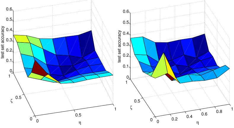
Figure 1: Comparison between two spectral penalties: the trace norm (left) and the Frobenius norm (right), each with an additional fixed rank constraint as described in Section 5.3. Each surface plot displays performance values over a range of η andζ values, all obtained using the synthetic data set. The minimal value achieved by the trace norm is 0.1222 and the one achieved by the rank constraint is 0.1540.

6.2 Results

We now summarize a number of experimental results for several of the aforementioned algorithms.

6.2.1 TRACENORMVERSUSLOW-RANK

In Figure 1, we present two performance plots over theη/ζparameter space, both obtained using the synthetic data set. The left plot displays the results when using the trace norm spectral penalty. Here we used the low rank decomposition formulation described in Section 5.3 which (by Proposition 5) has no local minima. The plot on the right uses the same rank-constrained formulation, but with a Frobenius norm penalty instead. The trace norm constrained algorithm performs slightly better. Moreover, best predictive performance is achieved in both cases in the middle of the square and not at any of the four corners.

6.2.2 KERNELLEARNING

(18)

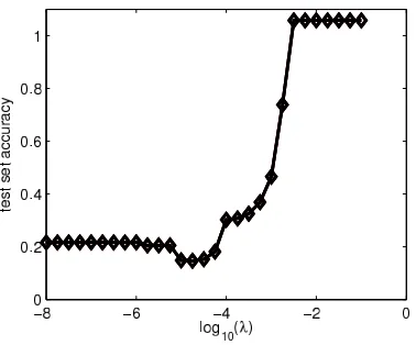
Figure 2: Learning the kernel: test set accuracy vs. regularization parameter. Minimum value is 0.14.

6.2.3 PERFORMANCE ON MOVIELENSDATA

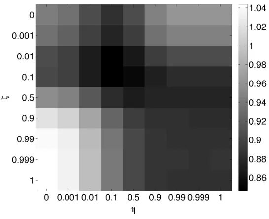
Figure 3 shows the predictive accuracy in RMSE on the MovieLens data set, obtained by 10-fold cross-validation. The heat plot provides some insight on the relative value, for both movies and users, of the given attribute kernels versus the simple identity kernels. The corners have higher values than some of the values inside the square, showing that the best balance between attribute and Dirac kernels is achieved forη,ζwell inside the interior of[0,1]×[0,1].

7. Conclusions

We have presented a method for solving a generalized matrix completion problem where we have attributes describing the matrix dimensions. The problem is formalized as the problem of inferring a linear compact operator between two general Hilbert spaces, which generalizes the classical finite-dimensional matrix completion problem. We introduced the notion of spectral regularization for operators, which generalizes various spectral penalizations for matrices, and we proved a general representer theorem for this setting. Various approaches, such as standard low rank matrix comple-tion, are special cases of our method. This framework is particularly relevant for CF applications where attributes are available for users and/or objects, and preliminary experiments confirm the benefits of our method.

An interesting direction of future research is to explore further the multi-task learning algorithm we obtained with low-rank constraint, and to study the possibility to derive on-line implementations that may better fit the need for large-scale applications where training data are continuously increas-ing. On the theoretical side, a better understanding of the effects of norm and rank regularizations and their interaction would be of considerable interest.

Acknowledgments

(19)

Figure 3: A heat plot of performance for a range of kernel parameter choices,ηandζ, using the MovieLens data set.

Appendix A. Compact Operators on Hilbert Spaces

In this appendix, we recall basic definitions and properties of Hilbert space operators. We refer the interested reader to general books (Brezis, 1980; Berlinet and Thomas-Agnan, 2003) for more details.

Let

X

and

Y

be two Hilbert spaces, with respective inner products denoted by hx,x′i_X and

Y

, (x⊗y)h=hy,hi_Yx.

We denote by

B0

(

Y

,

X

)the set of compact linear operators from

Y

to

X

, that is, the set of linear operators that map the unit ball of

Y

to a relatively compact set of

X

Y

,

X

).

• The operators F∈

B0

(

Y

,

X

)that satisfy:

∞

∑

i=1

σi(F)2<∞

are called Hilbert-Schmidt operators. They form a Hilbert space, denoted

B2

(

Y

,

X

), with inner producth·,·i_X_⊗_Y between basic tensor products given by:

x⊗y,x′⊗y′_X_⊗_Y =

x,x′_Xy,y′_Y . (18)

In particular, the Hilbert-Schmidt norm of an operator in

B2

(

Y

,

X

)is given by:

kFk2=

∞

∑

i=1

σi(F)2 !1₂

.

Another useful characterization of Hilbert-Schmidt operators is the following. Each linear operator F :

Y

B0

(

Y

,

X

)that satisfy:

∞

∑

i=1

σi(F)<∞

),

(21)

Appendix B. Proof of Theorem 3

We start with a general result about the decrease of singular values for compact operators composed with projection:

Lemma 7 Let

G

and

H

be two Hilbert spaces, H a compact linear subspace of

H

, andΠHdenote

the orthogonal projection onto H. Then for any compact operator F :

G

7→

H

it holds that:

∀i≥1, σi(ΠHF)≤σi(F).

Proof We use the classical characterization of the i-th singular value:

σi(F) = max

V∈Vi(G)x∈Vmin,kxkG=1

kFxk_H ,

where

V

i(

G

)denotes the set of all linear subspaces of

G

of dimension i. Now, observing that for

any x we havekΠHFxkH ≤ kFxkH proves the Lemma.

Given a training set of patterns(xi,yi)_i₌₁_,...,_N∈

X

×

,

X

), let us now consider the operator G=ΠXNFΠYN. By construction, F and G agree on the training patterns, in the sense that for i=1, . . . ,N:

hxi,GyiiX =

xi,ΠXNFΠYNyi

X =

Π

XNxi,FΠYNyi

X =hxi,FyiiX .

Therefore F and G have the same empirical risk:

RN(F) =RN(G). (19)

Now, by denoting F∗the adjoint operator, we can use Lemma 7 and the fact that the singular values of an operator and its adjoint are the same to obtain, for any i≥1:

σi(G) =σi(ΠXNFΠYN) ≤σi(FΠYN)

=σi(ΠYNF

∗₎

≤σi(F∗)

=σi(F).

This implies that the spectral penalty term satisfiesΩ(G)≤Ω(F). Combined with (19), this shows that if F is a solution to (12), then G=ΠXNFΠYN is also a solution. Observing that G∈

X

N⊗

Y

N concludes the proof of the first part of Theorem 3, resulting in (13).

We have now reduced the optimization problem in

B0

(

Y

,

X

)to a finite-dimensional optimiza-tion over the matrix α of size mX×mY. Let us now rephrase the optimization problem in this

finite-dimensional space.

Let us first consider the spectral penalty termΩ(F). Given the decomposition (13), the non-zero singular values of F as an operator are exactly the non-zero singular values ofαas a matrix, as soon as(u1, . . . ,umX)and v1, . . . ,vmY

(22)

be able to express the empirical risk RN(F)we must however consider a decomposition of F over

the training patterns, as:

F=

N

∑

i=1

N

∑

j=1

γi jxi⊗yj. (20)

In order to express the singular values from this expression let us introduce the Gram matrices K and G of the training patterns, that is, the N×N matrices defined for i,j=1, . . . ,N by:

Ki j=

xi,xj

X , Gi j=

yi,yj

Y .

We note that by definition the ranks of K and G are respectively mX and mY. Let us now

fac-torize these two matrices as K=X X⊤ and G=YY⊤, where X ∈RN×mX _{and Y} _∈_RN×mY _{are any}

square roots, for example, obtained by kernel PCA or incomplete Cholesky decomposition (Fine and Scheinberg, 2001; Bach and Jordan, 2005). The matrices X and Y provide a representation of the pattern in two orthonormal bases which we denote by(u1, . . . ,umX) and v1, . . . ,vmY

FN=diag(KγG) =diag

XαY⊤

.

We can now replace the empirical risk RN(FN)by RN diag XαY⊤

and the penaltyΩ(F)byΩ(α)

to deduce the optimization problem (14) from (12), which concludes the proof of Theorem 3.

Appendix C. Proof of Proposition 5

Since the function has compact level sets, we may assume that we are restricted to an open bounded subset ofRp×q_{where the second and first derivatives are uniformly bounded. We let denote C}_>₀

a common upper bound of all derivatives. The gradient of the function H is equal to∇H= ∇G_{∇G V}⊤U

, while the Hessian of H is the following quadratic form:

(23)

Without loss of generality, we may assume that the last columns of U and V are equal to zero (this can be done by rotation of U or V ). The zero gradient assumption implies that ∇G⊤U =0 and

∇GV=0. While if we take dU and dV with the first m−1 columns equal to zero, and last columns equal to arbitrary u and v, then the second term in the Hessian is equal to zero. The positivity of the first term implies that for all u and v, v⊤∇Gu≥0, that is, the gradient of G at N=UV⊤is equal to zero, and thus we get a stationary point and thus a global minimum of G.

References

J. Abernethy, F. Bach, T. Evgeniou, and J.-P. Vert. Low-rank matrix factorization with attributes. Technical Report N24/06/MM, Ecole des Mines de Paris, 2006.

Y. Amit, M. Fink, N. Srebro, and S. Ullman. Uncovering shared structures in multiclass classifica-tion. In Z. Ghahramani, editor, ICML ’07: Proceedings of the 24th International Conference on Machine Learning, pages 17–24, New York, NY, USA, 2007. ACM.

A. Argyriou, T. Evgeniou, and M. Pontil. Convex multi-task feature learning. Mach. Learn., 73(3): 243–272, 2008.

N. Aronszajn. Theory of reproducing kernels. Trans. Am. Math. Soc., 68:337 – 404, 1950.

F. R. Bach. Consistency of trace norm minimization. J. Mach. Learn. Res., 9:1019–1048, 2008.

F. R. Bach and M. I. Jordan. Predictive low-rank decomposition for kernel methods. In ICML ’05: Proceedings of the 22nd International Conference on Machine Learning, pages 33–40, New York, NY, USA, 2005. ACM.

F. R. Bach, G. R. G. Lanckriet, and M. I. Jordan. Multiple kernel learning, conic duality, and the SMO algorithm. In ICML ’04: Proceedings of the Twenty-first International Conference on Machine Learning, page 6, New York, NY, USA, 2004. ACM.

F. R. Bach, R. Thibaux, and M. I. Jordan. Computing regularization paths for learning multiple kernels. In L. K. Saul, Y. Weiss, and L. Bottou, editors, Adv. Neural. Inform. Process Syst. 17, pages 73–80, Cambridge, MA, 2005. MIT Press.

A. Berlinet and C. Thomas-Agnan. Reproducing Kernel Hilbert Spaces in Probability and Statistics. Kluwer Academic Publishers, 2003.

S. Boyd and L. Vandenberghe. Convex Optimization. Cambridge Univ. Press, 2003.

J. S. Breese, D. Heckerman, and C. Kadie. Empirical analysis of predictive algorithms for col-laborative filtering. In 14th Conference on Uncertainty in Artificial Intelligence, pages 43–52, Madison, W.I., 1998. Morgan Kaufman.

H. Brezis. Analyse Fonctionnelle. Masson, 1980.