Elasticity Tensors in Nematic Liquid Crystals

(1)

This article is published under the terms of the Creative Commons Attribution License 4.0 Author(s) retain the copyright of this article. Publication rights with Alkhaer Publications. Published at: http://www.ijsciences.com/pub/issue/2016-07/

DOI: 10.18483/ijSci.1117; Online ISSN: 2305-3925; Print ISSN: 2410-4477



Amelia Carolina Sparavigna

(Correspondence)



d002040@polito.it



+

Elasticity Tensors in Nematic Liquid Crystals

Amelia Carolina Sparavigna

1 _

1_{Department of Applied Science and Technology, Politecnico di Torino, Italy}

Abstract: The paper is discussing the contributions to the free energy of elastic distortions in a nematic liquid crystal. These contributions are here given by tensors, which are represented by means of the components of the director, the unit vector indicating the local average alignment of molecules, and by Kronecker and Levi-Civita symbols. The paper is also discussing the elasticity of the second order and its contribution in threshold phenomena.

Keywords: Liquid Crystals, Nematics, Elasticity, Continuum Theories

1. Introduction

The equation of Oseen-Frank, which is providing the free energy density in nematic liquid crystals [1,2], is representing the part of that energy density coming from an elastic deformation of the bulk of the material. In such approach, the terms depending on the deformations are multiplied by the three elastic constants (K11, K22, K33) of “splay”, “twist” and

“bend”. After, to this energy density, Nehring and Saupe added two terms having elastic constants of “mixed splay-bend” (K13) and of “saddle- splay” (K24)

[3] . These terms, which have K13, K24 as elastic

constants, are equivalent to contributions to the surface free energy of the material, because they are divergences of some vector functions of the director. These contributions to surface energy are relevant for nematic cells subjected to weak anchoring conditions [4-6].

The elastic constants previously mentioned are constants that multiply some scalar functions obtained from the director, the unit vector giving the local average alignment of the molecules, and from its derivatives, in the form of rotors and divergences. In this paper, we will discuss how the terms of the free energy density in nematic liquid crystals can be described by tensors, and how these tensors can be represented using the director components and the Kronecker and Levi-Civita symbols. This paper will also discuss the terms of the second order and their role in threshold phenomena [7,8].

2. The elastic deformation of a nematic

In an ideal nematic, the molecules are oriented, in average, along the director, the macroscopic unit vector n [9]. This alignment of molecules along a common direction is proper of the nematic phase,

which, in this manner, is characterized by an orientational order. This order disappears in the isotropic phase. To describe the nematic phase, a tensor order parameter is given as:













_



_i _j _ij

ij

Q

T

n

Q



3

1 )

(

(1)

In (1), i and j are indices of the Cartesian frame of reference; ni are the director components and δij the Kronecker symbol. Scalar Q depends on the temperature and goes to zero in the isotropic phase. Tensor Qij can be a function of the position vector r. Let us remember that in the macroscopic approach of the continuum mechanics, this position vector does not describe the positions of the single microscopic molecules.

If the order parameter is depending on position r, then we need to assume this dependence through the director as follow:













_



_i _j _ij

ij

Q

T

n

Q



3

1 )

(

)

(

)

(

)

(

r

(2)

http://www.ijSciences.com Volume 5 – July 2016 (07)

55

Oseen and Frank demonstrated that the density of the free energy given by distortions in the second order of n is represented by the three deformations:













]

[

2

1

2 3

2 2

2 1

n

rot

K

rot

K

div

K

f

d











(3)

In (3), K1 is the elastic constant of splay, K2 of twist

and K3 of bend. Since it is possible to have

deformations of pure splay, or of twist or bend, each of these elastic constants must be positive. If it were not so, the undistorted deformation would not be that having the minimum energy.

The elastic constants Ki have the dimensions of a force, as we can see, using pure dimensional analysis, from Eq.3 where we have [Energy/L3_{] = [}_K_][L─2_],

and L is a length. Then [Energy/L] = [K]. Let us note that n is a dimensionless quantity. K is of the order of U/a, where U means a typical energy of interaction between molecules (U ~ 2 Kcal/mole) and a is the molecular dimension of length (a ~ 14 Ǻ). So, we have [10]:

dyne

cm

erg

K

₇ 6

13

10

4 .

1

10

4 .

1



 







(4)

For the liquid crystal PAA about 120°C, it is K1 = 0.7

10─6dyne, K2 = 0.43 10─6dyne, K3 = 1.7 10─6dyne

[10].

Assuming K1= K2 = K3 = K, we obtain the

one-elastic-constant approximation:



 





2 2



2

1 n

n

rot

div

K

F

_d





(5)

To determine the contribution to the free energy coming from the elastic deformation, Oseen and Frank used the following approach [9]. Let us assume the z-axis along the direction of director n, the x-axis perpendicular to the director and y-axis perpendicular to x- and z-axes, oriented according the right-hand rule.

We can distinguish six elemental distortions, linked to the director variation. Therefore, the deformations of splay, bend and twist can be described by means of six derivatives:

4 2

6 3

1 5

/

;

/

;

/

;

/

a

x

n

a

y

n

a

z

n

a

z

n

a

x

n

a

y

n

y x

x y

























(6)

For small deformations, we have:

z

a

y

a

x

a

n

z

a

y

a

x

a

n

y x z

6 5 4

3 2 1

1 









(7)

Then, we can write the density of the free energy coming from the distortion of the nematic according to the Hooke law, as a quadratic function of the deformation:

6 ...,

,

2 ,

1 ,

;

2

1 







j

i

K

a

K

a

K

g

ji ij

j i ij i

i

(8)

In (8), there are six elastic parameters Ki and 36 elastic parameters Kij. Anyway, using symmetries

these numbers of parameter are reduced. For instance, the cylindrical symmetry of the nematic liquid crystal implies invariance for rotation about z-axis. So the energy is invariant during such rotation. Then, because of invariance for transformation x’= y, y’=– x, z’= z, we have only two independent Ki parameters

(K1, K2) and five independent Kij parameters (K11 ,K22 ,K33, K 24,K 12 ).

Moreover, we have the condition n = –n, which is telling that the director direction does not influence the features of the medium. In this case, it is necessary that transformation z’ =–z, y’ =–y, x’ =–x, does not change the deformation of the three- dimensional structure. So we need K1 and K13 being

zero. Also the mirror symmetry exists, and then, according to transformation x’ = x, y’ = –y, z’ = z, we find K2 and K12 being zero.

In this manner, in the elastic energy density of nematics we have just four coefficients: K11, K22, K33

and K24 . However, the term multiplied by coefficient

K24 is not proper of the bulk energy, because it is a

(3)

http://www.ijSciences.com Volume 5 – July 2016 (07)

56

]

)

(

)

(

)

(

[

2

1

2 6 3 33

2 4 2 22 2 5 1 11

a

K

a

K

a

K

g









(9)

We can write (9) using rotor and divergence of director:

]

)

(

)

(

)

(

[

2

1

2 33

2 22

2 11

n

rot

K

rot

K

div

K

g











(10)

In the case of cholesteric nematics,

K

₂



0

. An

additional contribution given by K2 n·rotn, is

required in the second term of (10). So, instead of 2

22

(

n rot

n

)

K



, we have

]

)

(

)

(

)

(

[

2

1

2 33

2 22 2 22

2 11

n

rot

K

rot

K

div

K

g











(10’)

In fact, squaring the second term, the contribution of (K2/K22)2is not relevant, because it does not depend

on the deformation. The ratio q0 = K2 /K22 is the

modulus of the wave-vector of the cholesteric helical structure, having pitch P0 =2π/q0. In the case

0

2



K

, the equilibrium configuration of the cholesteric nematic is that having a spontaneous twisted deformation.

3. Elastic energy density, given by the derivatives

ni,j = ∂ni / ∂xj

Following the Oseen – Frank approach, let us being more general. If the director n does not depend on position, the liquid crystal is undistorted and the free energy density is supposed equal to a certain quantity represented by f0, which is a quantity that does not change if the liquid crystals is subjected to a deformation.

If n = n(r), the nematic is deformed. Let f being the density of elastic energy which is created in the material. We have then that ni,j=∂ni /∂xj are different from zero. Let us suppose that these derivatives of n are enough for describing the distorted nematic, and then:

)

(

n

_i_,_j

f



(11)

If these derivatives are small, it is possible to consider a series in ni,j, so that:

l k j i ijkl j

i ij

o

E

n

K

n

f

_, _, _,

2

1 





(12)

In (129, the components of tensors E and K are given by:

o l k j i ijkl

o j i j

i

n

f

K

n

f

E

_

































, ,

2

,

;

(12’)

These quantities are evaluated with respect the undistorted configuration, which is also that having the minimum energy. In (12), we have used Einstein notation which implies summation on a set of indices;

for instance





j i

j i j i j

i j

i

n

E

n

E

,

, .

Let us write E and K, using combinations made by n, and the Kroneckerδij and Levi-Civita εijk symbols. Since in a nematic, n and ─n are equivalent, each

term in (2) must be even in n. Let us remember that, for what is concerning the Kronecker symbol, it is

1 

ij



, if i=j. It is



ij



0

if i≠j. In the case of the

Levi-Civita symbol, we have



_ijk



1

if i,j,k are in cyclic order;



ijk





1

if i,j,k are not in cyclic order.

Then, we have



_ijk



0

in the other cases. Moreover, the cross product of two vectors a and b

can be written as

a



b





_kij

a

_i

b

_j

e

_k, where ek is a unit vector of the three unit vectors representing a Cartesian frame of reference.

In the case of the rotor of the director, we can write it as:

k j i kij

n

rot

n





_,

e

(13)

Let us consider tensor E. We can represent its components as:

kij k ij

j i j

i

E

n

E

n

E



₁



₂





₃



(14)

But E1 = E2 = 0, because the nematic is not polar.

Moreover:

n

n rot

E

n

E

n

E

_i_j _i _j _k _{k ij} _i _j







₃ _,

,



(4)

http://www.ijSciences.com Volume 5 – July 2016 (07)

57

This is a pseudoscalar, being the nematic helicity [11,12]. Since the energy is a scalar,

n rot



n

can be present in it, when this contribution is squared or if the nematic is a cholesteric nematic. In this case, the material is spontaneously showing a deformed configuration of the fundamental state having the minimum energy.

For tensor K we have Kijkl=Kklij, because it is present in the term

K

_i_jkl

n

_i_,_j

n

_k_,_l; so we can write:

4567

123

C

K

_i _{jk l}





(16)

In (16), we have:

ik l j jl k i ij l k k l j i l k j i

n

K

n

K

n

K

n

K

n

K

C



* 3 3 * 2 2 1 123





jk il jl ik k l ij il k j jk l i

K

n

K

n

K

C



7 6 5 * 4 4 4567





Since ni ni = 1, we can see that in (16) just some terms survive. They are:





2 * 3 , , * 3 , , * 3

n

n rot

K

n

K

n

K

_j _l _ik _i _j _k_l _j _l _i _j _i _l







(I)





2

5 , ,

5

n

K

div

n

K



ij



kl i j kl



(II)

l j j l l k l k l k j i jk il l k j i jl ik

n

K

n

K

n

K

n

K

, , 7 , , 6 , , 7 , , 6









(III)

Let us demonstrate the first (I). Using the Levi-Civita symbol for the cross product, we have:



n



rot

n



k





kij

n

i



jlm

n

l,m

Note that we have to sum on j. So, the following relation exists: il km im kl jlm

kij











. Therefore:





i k i i i k i k i k i i i k i k

n

rot

, , , ,

)

(

2

1 _

_











n

We used the fact that the director is a unit vector and then the derivative of its modulus is zero. (II) and

(III) contain factor

2 n

_i

n

_i_,_j





_j

(

n

_i

n

_i

)



0

. Then,

all the terms we are re-writing in the following formula are null, so as their sum:

0

, , * 4 , , 4 , , 3 , , * 2 , , 2 , , 1 , , * 4 , , 4 , , 3 , , * 2 , , 2 , , 1









l k i l k j l j j i l i j k j i k i l k i i l k k k j i j i l k j i l k j i l k j i il k j l k j i jk l i l k j i jl k i l k j i ij l k l k j i kl j i l k j i l k j i

n

K

n

K

n

K

n

K

n

K

n

K

n

K

n

K

n

K

n

K

n

K

n

K



The surviving terms which are contributing to the elastic energy are:

l j j l j k j

k

n

K

n

K

div

K

rot

K

₃*

(

n



n

)

2



₅

(

n

)

2



₆ _, _,



₇ _, _, (17)

We have [7]:

2 2

, , ,

,

n

(

n

rot

n

)

(

n

rot

n

)

n

_k _j _k _j



_k _j _j_k









(18)

)

(

)

(

2

,

n

div

n

div

n

div

n

rot

n

_k _j _j_k









(19)

(5)

http://www.ijSciences.com Volume 5 – July 2016 (07)

58

)

(

)

(

)

)(

(

)

(

)

)(

(

7 6

2 6

* 3 2 6

2 7

6 5

n

rot

div

K

rot

K

rot

K

div

K















(20)

We can change the symbols for the coefficients, to see that this expression is that of the free energy density proposed by Oseen – Frank, with the saddle-splay term too.

)

(

)

(

)

(

2

1 )

(

2

1 )

(

2

1

24 22

2 33

2 22

2 11

n

rot

div

K

rot

K

rot

K

div

K

f

_Frank

















(21)

As previously told, K11, K22, K33 e K24 are the elastic constants of splay, twist, bend, and saddle-splay. The last term

in (21), if we consider the Gauss theorem, is a contribution to the surface energy. Then, the density energy of the bulk is depending on the three elastic constants of splay, twist and bend. If we consider also the helicity, the free energy becomes:

)

(

)

(

)

(

2

1 )

(

2

1 )

(

2

1

24 22

2 33

2 22

2 11

n

rot

div

K

rot

K

rot

K

div

K

rot

E

f

_o





















(22)

If we have not splay and bend, and only twist is present, Equation (22) is minimized by:

n

n rot

K

E

_

_

22

(23)

Then, in the case we have helicity (E ≠ 0), the configuration of the director which is minimizing the energy is a distorted one. As previously told, this happens in the cholesteric liquid crystals. From now on, we assume a nematic having E = 0.

4. The analysis of Nehring and Saupe

Let n be the director and ni,j, ni,jk the derivatives of first and second order. Let us suppose a free energy density depending on these derivatives

f



f



n

_i,_j

,

n

_i,_j_k



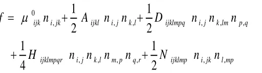
and represent it as a series of ni,j and ni,jk:

m l k j i m l k j i n m l k j i n m l k j i k j i k j i l k j i l k j

i

n

L

n

M

n

N

n

K

f



₀



_, _,



_,



_, _,



_, _, (24)

Being tensor L multiplying derivatives of the second order, it must be:

j k i k j

i

L



(25)

As we have done before, let us represent the components of tensors L, M and N, using n, δij and εijk. Let us start from L and determine its contribution to energy. Being n and ─n equivalent, the terms different from zero are:



j ik k ij



k j i k

j i k

j

i

L

n

L

n

L

n

L



₁



₂





₃







Then:

k j j k j

k k j j

j i i k

j i k j i k

j i k j

i

n

L

n

L

n

L

n

L

n

(6)

http://www.ijSciences.com Volume 5 – July 2016 (07)

59

Again, let us remember that ni ni = 1, and therefore:

k

j

i

j

i

k

i

j

i

n

_,



0 ;

_,





_,

(27)

Using (27), the first term in (26) becomes

n

_i

n

_j

n

_k

n

_i_,_j_k





(

n

_k

n

_i_,_k

)

2. The second becomes

n

_i

n

_i_,_j_j





n

_i_,_j

n

_i_,_j, The third is equivalent to:





2

, ,

, , ,

,ji

(

i j j

)

i ii j j

(

j j

)

j

i

n

div

n







n



Equation (26) can be written as



L

n

L

n

L

n



L

div



n div

n



n

L

_i_j_k _i_,_j_k





₁

(

_k _i_,_j

)

2



₂

(

_i_,_j

)

2



2

₃

(

_j_,_j

)

2



2

₃ (28)

We have already found the first three terms of (28), when we have discussed the tensor K. These terms can be added to those previously given. But in (28) we have a new term which is contributing to the surface term, like that having as elastic constant K24. This term is usually written with the constant K13, defined as the elastic constant of

splay-bend [13,14].

Supposing M = 0 and N = 0 , (24) becomes:

l k j i l k j i k j i k j

i

n

K

n

L

f



₀



_,



_, _, (29)

Therefore, after renormalizing the constants:























n





n



n

div

K

rot

div

K

rot

K

rot

K

div

K

f

_N_S

13 24

22

2 33

2 22

2 11

0

2

1 



















(30)

This is the free energy density of Nehring-Saupe [3]. However, we have also the terms coming from tensors M and N , to consider as sources of elastic constants, it they are different from zero. To dealt with them we need a second order analysis.

5. Second order analysis

We have seen in the previous section, that the free energy density, as given by Nehring and Saupe, including the term with elastic constant K13, is

originated from tensors K and L. However, other

terms exist that we have not yet discussed. To analyse them let us follow the approach given in [7]. In this reference, the free energy density is supposed a function of deformations as:



n

i j

n

i jk



f



_,

,

_,

That is, we assume as deformation sources, the first- and second-order derivatives of the director, generalizing the approach of the previous section.

The virtual variation δf of the density of the free energy f , close to equilibrium, can be described to the second order as:

jk i k j i j i j i jk i jk i j i j i

n

f

n

f

_, _, _,

, ,

,











(7)

http://www.ijSciences.com Volume 5 – July 2016 (07)

60

In (31), we find the variations of the first- and second-order derivatives of director n. In the linear theory of elasticity, in (31) we have to consider just the derivatives of the first-order, neglecting those of higher order. If the second-order is involved too, tensors λ, μ must be expanded in terms of the sources of deformation, ni,j and ni,jk. Therefore:



















q p m l q p m l k j i p m l p m l k j i m l m l k j i k j i k j i r q p m l k r q p m l k j i q p m l k q p m l k j i p m l k p m l k j i m l k m l k j i l k l k j i j i j i

n

O

n

N

n

M

n

H

n

D

n

C

n

B

n

A

, , , , 0 , , , , , , , , , 0





(32)

In (32) λ°, μ° are tensors depending just on the components ni but not dependent on ni,j and ni,jk, The same for tensors A, B, C, D, H, M, N and O.

Using (32) in (31), we see that only λ° is described by terms of the first order, whereas A, μ° have terms of the second order, B, C, M of the third and D, H, O of the fourth order.

We could ask ourselves if, in (32), it is also necessary a term of the form Fijklmp nk,lmp, which is of the same order of

D and H. In the approach we are following here, this term is not coming from the sources of deformation we are considering. And then, we do not include it, or other similar to it, in (32). The criterion is that λij and μijk are expanded only in terms of the deformation sources, as defined in (31).

Let us take into account the general property of the mixed second-order derivatives of continuous function g:

j i lm k lm k j

i

n

g

n

g

, , 2 , , 2







(33)

Equation (33) ensures that [7]:

klmijpq ijklmpq

klmij

ijklm

M

D

O

B



;



(33’)

Moreover, from symmetry considerations [7]:

mpk lijqr qrk lmpij ijk lqrmp ijmk lqr k lijmpqr ijk lmpqr pqk lmij ijk lmpq k lijmp ijmpk l ijk lmp k lij ijk l

H

D

C

A



;

(34)

Using (32) in (31), according to (33’) and (34), we have [7]:

mp l jk i ijklmp r q p m l k j i ijklmpqr q p lm k j i ijklmpq p m l k j i ijklmp lm k j i ijklm l k j i ijkl jk i ijk j i ij

n

N

n

H

n

D

n

C

n

B

n

A

n

f

, , , , , , , , , , , , , , , , , 0 , 0

2

1

4

1

2

1

3

1

2

1 









(35)

Usually, common nematics are not polar or chiral and then, in (35), odd terms in n and helicity

n rot



n

are not present. Therefore, for common nematics tensors λ°, B e C are null.

(8)

http://www.ijSciences.com Volume 5 – July 2016 (07)

61

mp l jk i ijklmp r

q p m l k j i ijklmpqr

q p lm k j i ijklmpq l

k j i ijkl jk

i ijk

n

N

n

H

n

D

n

A

n

f

, , ,

, , , ,

, ,

0

2

1

4

1

2

1

2

1 







(35’)

Let us expand tensors in (35’), using (ni,δij,εijk). After expanding the tensors, the terms that survive are (given in covariant form, that in using divergence and rotor):















n



n

rot

div

A

rot

A

rot

A

div

A

f

_A















4

2 3

2 2

2 1

(36a)















n





n



n

rot

div

rot

div

f



















2 4

2 3

2 2

2 1



(36b)

If we have only ni,j as source of deformation, (35’) becomes:

l k j i ijkl j

i

ij

n

A

n

f

0 _, _, _,

2

1 





(36’)

In this case, the term with K13 does not appear, in

agreement with the elastic theory of the first order as given by Oseen-Frank. Therefore, if we consider K13,

and also K24, we can ask ourselves what are the other

terms we need to consider too, to have the expression of f coherent to the second order approach given in [7]. In we assume (36a) and (36b), we have the well-known splay, twist and bend distortions coming from terms due to tensors μ° and A. However, we have many terms from tensors N, D and H (many of them are null because of the parity of n and pseudoscalarity of (n · rot n)). Let us note also that some terms are coming from both N and D, or from D and H, or from the three tensors at the same time.

In the three Tables I-III given after the References we show the contributions to the density of the free energy of a nematic liquid crystal coming from N, D

and H. In the first of the three tables, the terms are coming from N. In the second table we have contributions coming from D, andthosemarked by * are shared with N. In the third table we have the contributions to the density of the free energy coming from H (terms marked by * are shared with D,

whereas those marked by ** are shared with N and

D).

6. Second-order elasticity close to a threshold If we use for a nematic liquid crystal the theory of the first-order elasticity, we have only three constants to deal with. Whereas, if we use the theory of the second order, we have a quite larger number of elastic

constant. Then, the use of such theory turns out to be unworkable. In fact, the elasticity of the second order can become quite simple, when it is involved in a threshold phenomenon, when the nematic is changing its configuration from an undistorted to a distorted one.

Let us remember that the most common experimental condition to study the nematic is that of creating a cell composed by two plane-parallel glass slides, spaced a few microns, in which the nematic is inserted by capillarity. The two inner surfaces of the cell may have the same or different treatments, in order to induce the desired nematic configuration (planar, homeotropic or hybrid). The cell can be placed in a thermostat with appropriate optical windows for the observation under polarized microscopy of the phases or of the material configurations.

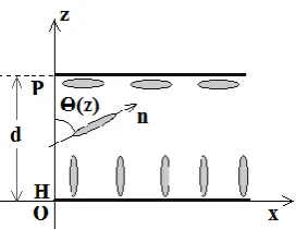
Let us consider a flat deformation of the nematic, that is, one which is obtained for example in a cell with opposite conditions, homeotropic on one of the walls and planar on to the other (this is the so-called hybrid HAN-cell. We can use a frame of reference (x,z) with the origin on the wall with homeotropic anchoring, the x-axis parallel to that wall, and the z-axis perpendicular to it.

(9)

http://www.ijSciences.com Volume 5 – July 2016 (07)

62

lower wall. In the intermediate part of the cell, the director forms an angle different from 0° and from 90°, with respect the z-axis.

Figure 1: Configuration of the molecules at the walls of a HAN cell in strong anchoring conditions.

Locally, the director n is given by:

n = i sin(Ө) + k cos(Ө) (37)

In (37), Ө(z) is the angle shown in the Figure 1. Vectors i and k are the unit vectors of axes.

If we imagine to decrease the cell thickness d, the deformed configuration becomes unstable and the cell, if we suppose that the planar anchoring is stronger than the homeotropic one, assumes the planar configuration. Or, if we assume the homeotropic anchoring stronger, the cell assumes the homeotropic configuration. The transition that occurs in the HAN cell, when we are reducing the thickness of the liquid crystal, is from a distorted configuration to the undistorted planar (P) or homeotropic (H)

configuration (see Figure 2).

Figure 2: Decreasing the cell thickness, we can see the distorted HAN configuration becoming a planar or homeotropic undistorted configuration shown on the right of the image.

In order to describe the occurrence of a limit for the mechanical stability of the HAN cell, due to the decrease of the cell thickness d, the free energy density must be given as a function of angle Ө. Close the threshold of the passage from the HAN configuration to the undistorted P or H configurations, we have Ө changing its value. However, the value of this angle depends on the positon of the director in the cell, that is, on z. So let us take as the parameter for studying the problem, the maximum angle assumed by the director with respect to z-axis and call it Өmax. If the

planar anchoring is strong, this angle can also be of 90°. In fact, we can think the angle Ө as a function of z, and therefore as a function Ө = Өmaxg(z/d).

Now, let us consider some terms from Tables I-III, and write them in covariant form [7]:

4 ,

, , , 2

2 ,

, , ,

2 2 ,

, 2 ,

,

)

(

;

)

(

)

(

;

)

(

n

rot

n

div

grad

n

p l m l k i j i p m k j l

k l k j i j i

kk i jj i kj

k ij i















(38)

Using (37), these terms become:





2 2

2 4

2 2

sin

2 sin

cos



















































   

n

div

grad

(39a)

 

4 2

2 2































n

  (39b)





4

2 2



















n



(10)

http://www.ijSciences.com Volume 5 – July 2016 (07)

63





4 4 4

cos



















n



n

rot

(39d)

In (39a)-(39d), we used





d

/

dz



. Let us suppose a transition from HAN to H configuration. Near the threshold,

Өmax0, and then the contributions of the smallest order in Өmax are coming from the term

2















in (39b). Let us

stress that 2















is of the second order in Өmax, whereas the other contributions vanish more rapidly, when Өmax

goes to zero. As a consequence, we have an additional term to the free energy density which can be written as:

2 * 2 2 *

)

(

















n

K



K

In the framework of the theory of elasticity here discussed, only K* isthe new elastic constant of the second order which survives in a threshold phenomenon. In this case, the free energy density becomes:





2 2 * 24

22 13

2 33

2 22

2 11

)

(

)

(

)

(

)

(

)

(

)

(

)

(

2

1 n

n























K

rot

div

K

div

K

rot

K

rot

K

div

K

f

(40)

Let us note that the first five elastic constants have dimensions of energy divided by length; the elastic constant K* is an energy times a length. Let us evaluate its order as made for (4). We have [Energy][L─3] = [K*][L─4], where L is a length. Then [Energy][L] = [K*] and then the order of K* is U·a. If U is the typical energy of molecular interaction and a the typical length of molecules, we have:

2 20

20 7

13

10

2

10

2

10

4 .

1

10

4 .

1 *

erg

cm

erg

cm

dyne

cm

K





























Let us consider the deformation as Ө = Өmax g(z/d). Let ς=z/d be the dimensionless variable. Deformation are of the

following orders:

 



, max 2 2

2

, max

1

1 g

d

dz

d

dz

d

g

d

dz

d

dz

d











































 



(41)

We can define ξ the dimensionless derivative (slope) of g with respect to ς, that is

g

_,_, and the dimensionless curvature κ of this function as approximated by

g

_,_ . We will have:





_max

2 max

1 ;

1 









 

d

(11)

http://www.ijSciences.com Volume 5 – July 2016 (07)

64

2 2 max 4 2 2 max 2

*

_









d

K

d

K

f

(42)

We can evaluate the thickness d of the cell for which the term with K* becomes relevant. This happens when the two terms in (42), are comparable:

2 2 2

2 max 4

2 2

max 2

2

_*







K

d

K

d

K

_

_

_

_

_

We have that the thickness d for which K* is relevant depends on the square ratio between curvature and slope of the deformation, a ratio which is depending on the anchoring conditions of the cell. As a conclusion we can tell that, in certain anchoring conditions of the cell, the term with elastic constant K* cannot be neglected in evaluating the threshold value of the cell thickness.

References

1) Oseen, C. W. (1933). The theory of liquid crystals. Transactions of the Faraday Society, 29(140), 883-899. DOI: http://dx.doi.org/10.1039/tf9332900883

2) Frank, F. C. (1958). I. Liquid crystals. On the theory of liquid crystals. Discussions of the Faraday Society, 25, 19-28. DOI: http://dx.doi.org/10.1039/df9582500019

3) Nehring, J., & Saupe, A. (1972). Calculation of the elastic constants of nematic liquid crystals. J. Chem. Phys. 56, 5527-5529 DOI: http://dx.doi.org/10.1063/1.1677071

4) Sparavigna, A., Lavrentovich, O. D., & Strigazzi, A. (1994). Periodic stripe domains and hybrid-alignment regime in nematic liquid crystals: Threshold analysis. Physical Review E, 49(2), 1344. DOI: http://dx.doi.org/10.1103/physreve.49.1344

5) Sparavigna, A., Komitov, L., Stebler, B., & Strigazzi, A. (1991). Static splay-stripes in a hybrid aligned nematic layer. Molecular Crystals and Liquid Crystals 207(1), 265-280. DOI: http://dx.doi.org/10.1080/10587259108032105 6) Sparavigna, A., Komitov, L., Lavrentovich, O. D., &

Strigazzi, A. (1992). Saddle-splay and periodic instability in a hybrid aligned nematic layer subjected to a normal magnetic

field. Journal de Physique II, 2(10), 1881-1888. DOI: http://dx.doi.org/10.1051/jp2:1992241

7) Barbero, G., Sparavigna, A., & Strigazzi, A. (1990). The structure of the distortion free-energy density in nematics: second-order elasticity and surface terms. Il Nuovo Cimento D, 12(9), 1259-1272. DOI: http://dx.doi.org/10.1007/bf02450392

8) Sparavigna, A., Komitov, L., & Strigazzi, A. (1991). Hybrid Aligned Nematics and second order elasticity. Physica Scripta, 43(2), 210. DOI: http://dx.doi.org/10.1088/0031-8949/43/2/017

9) Stephen, M. J., & Straley, J. P. (1974). Physics of liquid crystals. Reviews of Modern Physics, 46(4), 617-704. DOI: http://dx.doi.org/10.1103/revmodphys.46.617

10) De Gennes, P. G., & Prost, J. (1995). The Physics of Liquid Crystals, Clarendon Press. ISBN: 0198517858, 9780198517856

11) Sparavigna, A. C. (2012). Distortional Lifshitz vectors and helicity in nematic free energy density. arXiv preprint arXiv:1207.2918.

12) Sparavigna, A. C. (2013). Distortional Lifshitz vectors and Helicity in nematic free energy density, International Journal of Sciences 07(2013):54-59. DOI: http://dx.doi.org/10.18483/ijsci.211

13) Lavrentovich, O. D., & Pergamenshchik, V. M. (1995). Patterns in thin liquid crystal films and the divergence (“surfacelike”) elasticity. International Journal of Modern Physics B, 9, 2389-2437. DOI: http://dx.doi.org/10.1142/9789812831101_0008

14) Pergamenshchik, V. M., Subacius, D., & Lavrentovich, O. D. (1997). K13-induced deformations in a nematic liquid crystal:

(12)

http://www.ijSciences.com Volume 5 – July 2016 (07)

65