Fast Iterative Kernel Principal Component Analysis
Simon G ¨unter [email protected]
Nicol N. Schraudolph [email protected]
S.V.N. Vishwanathan [email protected]
Research School of Information Sciences and Engineering Australian National University –and–
Statistical Machine Learning Program National ICT Australia, Locked Bag 8001 Canberra ACT 2601, Australia
Editor: Aapo Hyvarinen
Abstract
We develop gain adaptation methods that improve convergence of the kernel Hebbian algorithm (KHA) for iterative kernel PCA (Kim et al., 2005). KHA has a scalar gain parameter which is either held constant or decreased according to a predetermined annealing schedule, leading to slow convergence. We accelerate it by incorporating the reciprocal of the current estimated eigenvalues as part of a gain vector. An additional normalization term then allows us to eliminate a tuning parameter in the annealing schedule. Finally we derive and apply stochastic meta-descent (SMD) gain vector adaptation (Schraudolph, 1999, 2002) in reproducing kernel Hilbert space to further speed up convergence. Experimental results on kernel PCA and spectral clustering of USPS digits, motion capture and image denoising, and image super-resolution tasks confirm that our methods converge substantially faster than conventional KHA. To demonstrate scalability, we perform kernel PCA on the entire MNIST data set.
Keywords: step size adaptation, gain vector adaptation, stochastic meta-descent, kernel Hebbian algorithm, online learning
1. Introduction
Principal components analysis (PCA) is a standard linear technique for dimensionality reduction.
Given a matrixX∈Rn×l of l centered, n-dimensional observations, PCA performs an
eigendecom-position of the covariance matrixQ:=XX>. The r×n matrixW whose rows are the eigenvectors
ofQassociated with the r≤n largest eigenvalues minimizes the least-squares reconstruction error
kX−W>W XkF, (1)
wherek · kF is the Frobenius norm.
As it takes O(n2l)time to computeQand O(n3) time to eigendecompose it, PCA can be
pro-hibitively expensive for large amounts of high-dimensional data. Iterative methods exist that do
not computeQexplicitly, and thereby reduce the computational cost to O(rn)per iteration. They
assume that each individual observationxis drawn from a statistical distribution1, and the aim is
to maximize the variance ofy:=W x, subject to some orthonormality constraints on the weight
matrixW. In particular, we obtain the so-called hierarchical PCA network if we assume that the
ith row ofW must have unit norm and must be orthogonal to the jth row, where j=1, . . . ,i−1
(Karhunen, 1994). By using Lagrange multipliers to incorporate the constraints into the objective,
we can rewrite the merit function J(W)succinctly as (Karhunen and Joutsensalo, 1994):
J(W) =E[x>W>W x] +12tr[Λ(W W>−I)], (2)
where the Lagrange multiplier matrixΛis constrained to be lower triangular. Taking gradients with
respect toW and setting to zero yields
∂WJ(W) =E[W x]x>+ΛW =0. (3)
As a consequence of the KKT conditions (Boyd and Vandenberghe, 2004), at optimality
Λ(W W>−I) =0. (4)
Right multiplying (3) byW>, using (4), and noting thatΛmust be lower triangular yields
Λ=−lt(E[W x]x>W>) =−lt(E[y]y>), (5)
where lt(·)makes its argument lower triangular by zeroing all elements above the diagonal.
Plug-ging (5) into (3) and stochastically approximating the expectationE[y]with its instantaneous
esti-mateyt :=Wtxt, wherext ∈Rnis the observation at time t, yields
∂WtJ(W) =ytx>t −lt(ytyt>)Wt. (6)
Gradient ascent in (6) gives the generalized Hebbian algorithm (GHA) of Sanger (1989):
Wt+1=Wt+ηt[ytx>t −lt(ytyt>)Wt]. (7)
For an appropriate scalar gain,ηt, (7) will tend to converge to the principal component solution as
t→∞; though its global convergence is not proven (Kim et al., 2005).
A closely related algorithm by Oja and Karhunen (1985, Section 5) omits the lt operator:
Wt+1=Wt+ηt[ytx>t −ytyt>Wt]. (8)
This update is also motivated by maximizing the variance ofW x subject to orthonormality
con-straints onW. In contrast to GHA it requires the ithrow ofW to be orthogonal to all other rows of
W, that is, thatW be orthonormal. The resulting algorithm converges to an arbitrary orthonormal
basis—not necessarily the eigen-basis—for the subspace spanned by the first r eigenvectors. One can do better than PCA in minimizing the reconstruction error (1) by allowing
nonlin-ear projections of the data into r dimensions. Unfortunately such approaches often pose difficult
nonlinear optimization problems. Kernel methods (Sch ¨olkopf and Smola, 2002) provide a way to incorporate non-linearity without unduly complicating the optimization problem. Kernel PCA (Sch¨olkopf et al., 1998) performs an eigendecomposition on the kernel expansion of the data, an
l×l matrix. To reduce the attendant O(l2) space and O(l3) time complexity, Kim et al. (2005)
Both GHA and KHA are examples of stochastic approximation algorithms, whose iterative up-dates employ individual observations in place of—but, in the limit, approximating—statistical prop-erties of the entire data. By interleaving their updates with the passage through the data, stochastic approximation algorithms can greatly outperform conventional methods on large, redundant data sets, even though their convergence is comparatively slow.
Both GHA and KHA updates incorporate a scalar gain parameterηt, which is either held fixed or
annealed according to some predefined schedule. Robbins and Monro (1951) were first to establish
conditions on the sequence ofηt that guarantee the convergence of many stochastic approximation
algorithms on stationary input. A widely used annealing schedule (Darken and Moody, 1992) that obeys these conditions is
ηt =
τ
t+τη0, (9)
where t denotes the iteration number, andη0,τare positive tuning parameters. τ determines the
length of an initial search phase with near-constant gain (ηt ≈η0for tτ), before the gain decays
asymptotically as τ/t (for t τ) in the annealing phase (Darken and Moody, 1992). For
non-stationary inputs (e.g., in a online setting) Kim et al. (2005) suggest a small constant gain.
Here we propose the inclusion of a gain vector in the KHA, which provides each estimated eigenvector with its individual gain parameter. In Section 3.1 we describe our KHA/et* algorithm, which sets the gain for each eigenvector inversely proportional to its estimated eigenvalue, in ad-dition to using (9) for annealing. Our KHA/et algorithm in Section 3.3 adad-ditionally multiplies the
gain vector by the length of the vector of estimated eigenvalues; this allows us to eliminate theτ
tuning parameter.
We then derive and apply the stochastic meta-descent (SMD) gain vector adaptation technique (Schraudolph, 1999, 2002) to KHA/et* and KHA/et to further speed up their convergence. Our resulting KHA-SMD* and KHA-SMD methods (Section 4.2) adapt gains in a reproducing kernel Hilbert space (RKHS), as pioneered in the recent Online SVMD algorithm (Vishwanathan et al., 2006). The application of SMD to the KHA is not trivial; a naive implementation would require
O(rl2)time per update. By incrementally maintaining and updating two auxiliary matrices we
re-duce this cost to O(rl). Our experiments in Section 5 show that the combination of preconditioning
by the estimated eigenvalues and SMD can yield much faster convergence than either technique applied in isolation.
The following section summarizes the KHA, before we provide our eigenvalue-based gain mod-ifications in Section 3. Section 4 describes SMD and its application to the KHA. We report the results of our experiments with these algorithms in Section 5, then conclude with a discussion of our findings.
2. Kernel Hebbian Algorithm
Kim et al. (2005) adapt Sanger’s (1989) GHA algorithm to work with data mapped into a
reproduc-ing kernel Hilbert space (RKHS)
H
via a feature map Φ:X
→H
(Sch ¨olkopf and Smola, 2002).Here
X
is the input space, andH
andΦare implicitly defined by the kernel k :X
×X
→H
withthe property∀x,x0∈
X
: k(x,x0) =hΦ(x),Φ(x0)iH, whereh·,·iH denotes the inner product inH
.LetΦdenote the transposed data vector in feature space:
This assumes a fixed set of l observations whereas GHA relies on an infinite sequence of
observa-tions for convergence. Following Kim et al. (2005), we use an indexing function p :N→Zl which
concatenates random permutations ofZl to reconcile this discrepancy. Our implementations loop
through a fixed data set, permuting it anew before each pass.
PCA, GHA, and hence KHA all assume that the data is centered. Since the kernel which maps the data into feature space does not necessarily preserve such centering, we must re-center the data in feature space:
Φ0:=Φ−MΦ, (11)
whereM denotes the l×l matrix with entries all equal to 1/l. This is achieved by replacing the
kernel matrixK:=ΦΦ> (that is,[K]i j:=k(xi,xj)) by its centered version
K0:=Φ0Φ0>= (Φ−MΦ)(Φ−MΦ)>
=ΦΦ>−MΦΦ>−ΦΦ>M>+MΦΦ>M> (12)
=K−MK−(MK)>+MKM.
Since all rows ofMKare identical (as are all elements ofMKM) we can pre-calculate each row
in O(l2)time and store it in O(l)space to efficiently implement operations with the centered kernel.
The kernel centered on the training data is also used when testing the trained system on new data. From kernel PCA (Sch ¨olkopf et al., 1998) it is known that the principal components must lie in the span of the centered data in feature space; we can therefore express the GHA weight matrix
asWt =AtΦ0, whereAis an r×l matrix of expansion coefficients, and r the desired number of
principal components. The GHA weight update (7) thus becomes
At+1Φ0=AtΦ0+ηt[ytΦ0(xp(t))>−lt(ytyt>)AtΦ0], (13)
where lt(·)extracts the lower triangular part of its matrix argument (by setting all matrix elements
above the diagonal to zero), and
yt:=WtΦ0(xp(t)) =AtΦ0Φ0(xp(t)) =Atk0p(t), (14)
using ki0 to denote the ith column of the centered kernel matrix K0. Since we have Φ0(xi)> =
e>i Φ0, whereei is the unit vector in direction i, (13) can be rewritten solely in terms of expansion
coefficients as
At+1=At +ηt[yte>p(t)−lt(ytyt>)At]. (15)
Introducing the update coefficient matrix
Γt:=yte>
p(t)−lt(ytyt>)At (16)
we obtain the compact update rule
At+1=At+ηtΓt. (17)
In their experiments, Kim et al. (2005) employed the KHA update (17) with a constant scalar gain
ηt =η0; they also proposed letting the gain decay as ηt =η0/t. Our implementation (which we
denote KHA/t) employs the more general (9) instead, from which anη0/(t+1)decay is obtained
3. Gain Decay with Reciprocal Eigenvalues
Consider the termytxt>=Wtxtxt>appearing on the right-hand side of the GHA update (7). At the
desired solution, the rows ofWt contain the principal components, that is, the leading eigenvectors
ofQ=XX>. The elements ofytthus scale with the associated eigenvalues ofQ. Large differences
in eigenvalues can therefore lead to ill-conditioning (hence slow convergence) of the GHA; the same holds for the KHA.
We counteract this problem by furnishing the KHA with a gain vectorηt ∈Rr+ that provides
each eigenvector estimate with its individual gain parameter; we will discuss how to setηt below.
The update rule (17) thus becomes
At+1=At+diag(ηt)Γt, (18)
where diag(·)maps a vector into a diagonal matrix.
3.1 The KHA/et* Algorithm
To improve the KHA’s convergence, we setηt proportional to the reciprocal of the estimated
eigen-values. Letλt∈Rr+denote the vector of eigenvalues associated with the current estimate of the first
r eigenvectors. Our KHA/et* algorithm sets the ith component ofηt to [ηt]i=
1
[λt]i
τ
t+τη0, (19)
withη0andτpositive tuning parameters as in (9) before. Since we do not want the annealing phase
to start before we have seen all observations at least once, we tuneτin small integer multiples of
the data set size l.
KHA/et* thus conditions the KHA update by proportionately decreasing (increasing) the gain
(19) for rows ofAtassociated with large (small) eigenvalues. A similar approach (with a simple 1/t
gain decay) was applied by Chen and Chang (1995) to GHA for neural network feature selection.
3.2 Calculating the Eigenvalues
The above update (19) requires the first r eigenvalues of K0—but the KHA is an algorithm for
estimating these eigenvalues and their associated eigenvectors in the first place. The true eigenvalues are therefore not available at run-time. Instead we use the eigenvalues associated with the KHA’s
current eigenvector estimate inAt, computed as
[λt]i=k
K0[At]>i∗k2 k[At]>i∗k2
, (20)
where[At]i∗denotes the ithrow ofAt, andk·k2the 2-norm of a vector. This can be stated compactly
as
λt =
s
diag(AtK0(AtK0)>)
diag(AtA>t )
, (21)
where the division and square root operation are performed element-wise, and diag(·)applied to a
The main computational effort for calculating λt lies in computing AtK0, which—if done
naively—is quite expensive: O(rl2). Fortunately it is not necessary to do this at every iteration,
since the eigenvalues evolve but gradually. We empirically found it sufficient to update λt and
ηt only once after each pass through the data, that is, every l iterations—see Figure 4. Finally,
Section 4.2 below introduces incremental updates (33) and (34) that reduce the cost of calculating
AtK0to O(rl).
3.3 The KHA/et Algorithm
Theτparameter of the KHA/et* update (19) above determines at what point in the iterative kernel
PCA we gradually shift from the initial search phase (with near-constant ηt) into the asymptotic
annealing phase (with ηt near-proportional to 1/t). It would be advantageous if this parameter
could be determined adaptively (Darken and Moody, 1992), obviating the manual tuning required in KHA/et*.
One way to achieve this is to have some measure of progress counteract the gain decay: As long as we are making rapid progress, we are in the search phase, and do not want to decrease the
gains; when progress stalls it is time to start annealing them. A suitable measure of progress iskλtk,
the length of the vector of eigenvalues associated with our current estimate of the eigenvectors, as calculated via (20) above. This quantity is maximized by the true eigenvectors; in the KHA it tends to increase rapidly early on, then approach the maximum asymptotically.
Our KHA/et algorithm fixes the gain decay schedule of KHA/et* at τ=l, but multiplies the
gains bykλtk:
[ηt]i=k λtk [λt]i
l
t+lη0. (22)
The rapid early growth ofkλtkthus serves to counteract the gain decay until the leading eigenspace
has been identified. Asymptoticallykλtkapproaches its (constant) maximum, and so the gain decay
will ultimately dominate (22). This achieves an effect comparable to an “adaptive search then
con-verge” (ASTC) gain schedule (Darken and Moody, 1992) while eliminating theτtuning parameter.
Since (19) and (22) can both be expressed as
[ηt]i=
ˆ ηt [λt]i
, (23)
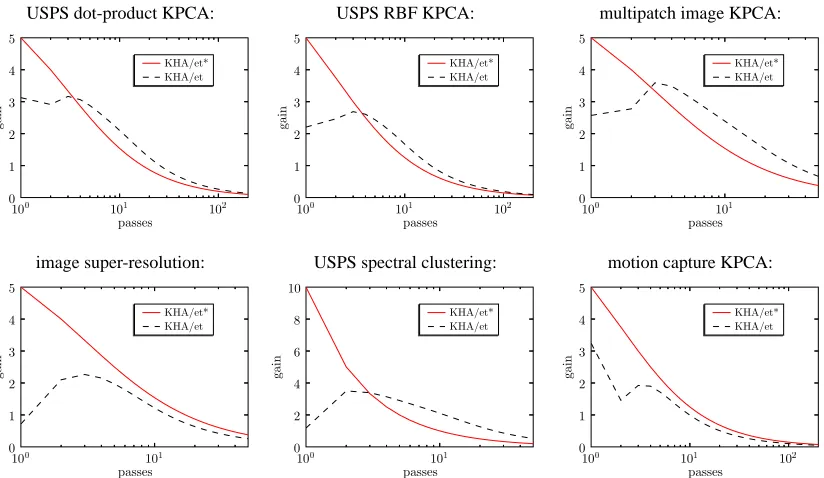
for particular choices of ˆηt, we can compare the gain vectors used by KHA/et* and KHA/et by
monitoring how they evolve the scalar ˆηt; this is shown in Figure 1 for all experiments reported
in Section 5. We see that although both algorithms ultimately anneal ˆηt in a similar fashion, their
behavior early on is quite different: KHA/et keeps a lower initial gain roughly constant for a
pro-longed search phase, whereas KHA/et* (for the optimal choice ofτ) starts decaying ˆηt far earlier,
albeit from a higher starting value. In Section 5 we shall see how this affects the performance of the two algorithms.
4. KHA with Stochastic Meta-Descent
USPS dot-product KPCA: USPS RBF KPCA: multipatch image KPCA:
image super-resolution: USPS spectral clustering: motion capture KPCA:
Figure 1: Comparison of gain ˆηt (23) between KHA/et* and KHA/et in all applications reported in
Section 5, at individually optimal values ofη0and (for KHA/et*)τ.
history of parameter updates so as to optimize convergence. We briefly review gradient-based gain adaptation methods, then derive and implement Schraudolph’s (1999; 2002) stochastic meta-descent (SMD) algorithm for both KHA/et* and KHA/et, focusing on the scalar form of SMD that can be used in an RKHS.
4.1 Scalar Stochastic Meta-Descent
Let V be a vector space,θ∈V a parameter vector, and J : V→Rthe objective function which we
would like to optimize. We assume that J is twice differentiable almost everywhere. Denote by
Jt : V →Rthe stochastic approximation of the objective function at time t. Our goal is to find θ
such thatEt[Jt(θ)]is minimized. We adaptθvia the stochastic gradient descent
θt+1=θt−eρtgt, where gt =∂θtJt(θt), (24)
using ∂θt as a shorthand for ∂∂θ
θ=θt
. Stochastic gradient descent is sensitive to the value of the
log-gainρt ∈R: If it is too small, (24) will take many iterations to converge; if it is too large, (24)
may diverge.
One solution is to adaptρtby a simultaneous meta-level gradient descent. Thus we could seek to
∂ρtJt+1(θt+1). Using the chain rule and (24) we find
ρt+1=ρt−µ∂ρtJt+1(θt+1)
=ρt−µ[∂θt+1Jt+1(θt+1)]>∂ρtθt+1 (25) =ρt+µ eρtgt>+1gt,
where the meta-gain µ≥0 is a scalar tuning parameter. Intuitively, the gain adaptation (25) is driven
by the angle between successive gradient measurements: If it is less than 90◦, theng>t+1gt >0, and
ρt will be increased. Conversely, if the angle is more than 90◦(oscillating gradient), thenρt will be
decreased becausegt>+1gt <0. Thus (25) serves to decorrelate successive gradients, which leads to
improved convergence of (24).
One shortcoming of (25) is that the decorrelation occurs only across a single time step, mak-ing the gain adaptation overly sensitive to spurious short-term correlations in the data. Stochastic
meta-descent (SMD; Schraudolph, 1999, 2002) addresses this issue by employing an exponentially
decaying trace of gradients across time:
ρt+1=ρt−µ t
∑
i=0
ξi∂
ρt−iJt+1(θt+1) =ρt−µ[∂θt+1Jt+1(θt+1)]>
t
∑
i=0
ξi∂ρ
t−iθt+1 (26) =:ρt−µgt>+1vt+1,
where the vectorvt+1∈V characterizes the dependence ofθt+1on its gain history over a time scale
governed by the decay factor 0≤ξ≤1, a scalar tuning parameter.
To computevt+1efficiently, we expandθt+1in terms of its recursive definition (24):
vt+1:= t
∑
i=0
ξi∂
ρt−iθt+1 =
t
∑
i=0
ξi∂
ρt−iθt− t
∑
i=0
ξi∂
ρt−i[e
ρtg
t] (27)
≈ξvt−eρt(gt+∂θtgt t
∑
i=0
ξi∂
ρt−iθt).
Here we have used∂ρtθt =0, and approximated
t
∑
i=1
ξi∂
ρt−iρt ≈0, (28)
which amounts to stating that the log-gain adaptation must be in equilibrium on the time scale
determined by ξ. Noting that ∂θtgt is the Hessian Ht of Jt(θt), we arrive at the simple iterative
update
vt+1=ξvt−eρt(gt+ξHtvt). (29)
Since the initial parametersθ0do not depend on any gains,v0=0. Note that for ξ=0 (29) and
Computation of the Hessian-vector product Htvt would be expensive if done naively.
For-tunately, efficient methods exist to calculate this quantity directly without computing the Hessian (Pearlmutter, 1994; Griewank, 2000; Schraudolph, 2002). In essence, these methods work by
prop-agatingvas a differential (i.e., directional derivative) through the gradient computation:
dθt :=vt ⇒ Htvt :=dgt. (30)
In other words, if we set the differential dθt of the parameter vector tovt, then the resulting
differ-ential of the gradientgt (a function ofθt) is the Hessian-vector productHtvt. We will see this at
work for the case of the KHA in (36) below.
4.2 SMD for KHA
The KHA update (18) can be viewed as r coupled updates in RKHS, one for each row ofAt, each
associated with a scalar gain. To apply SMD here we introduce an additional log-gain vectorρt∈Rr
At+1=At+ediag(ρt)diag(ηt)Γt. (31)
(The exponential of a diagonal matrix is obtained simply by exponentiating the individual diagonal entries.) We are thus applying SMD to KHA/et, that is, to a gradient descent preconditioned by the reciprocal estimated eigenvalues. SMD will happily work with such a preconditioner, and benefit from it.
In an RKHS, SMD adapts a scalar log-gain whose update is driven by the inner product between the gradient and a differential of the system parameters, all in the RKHS (Vishwanathan et al., 2006).
In the case of KHA,ΓtΦ0can be interpreted as the gradient in the RKHS of the merit function (2)
maximized by KHA. Therefore SMD’s adaptation of ρt in (31) is driven by the diagonal entries
ofhΓtΦ0,BtΦ0iH, whereBt :=dAt denotes the r×l matrix of expansion coefficients for SMD’s
differential parameters, analogous to thevvector in Section 4.1:
ρt =ρt−1+µ diag(
ΓtΦ0,BtΦ0 H)
=ρt−1+µ diag(ΓtΦ0Φ0>Bt>) (32) =ρt−1+µ diag(ΓtK0Bt>).
Naive computation of ΓtK0 in (32) would cost O(rl2)time, which is prohibitively expensive for
large l. We can, however, reduce this cost to O(rl)by noting that (16) implies that
ΓtK0=yte>
p(t)K0−lt(yty>t )AtK0
=ytk0>p(t)−lt(ytyt>)AtK0, (33)
where the r×l matrixAtK0can be stored and updated incrementally via (31):
At+1K0=AtK0+ediag(ρt)diag(ηt)ΓtK0. (34)
The initial computation ofA1K0 still costs O(rl2)in general but is affordable as it is performed
only once. Alternatively, the time complexity of this step can easily be reduced to O(rl)by making
Finally, we apply SMD’s standard update (29) of the differential parameters:
Bt+1=ξBt+ediag(ρt)diag(ηt) (Γt+ξdΓt). (35)
The differential dΓt of the gradient, analogous to dgt in (30), can be computed by applying the rules
of calculus:
dΓt=d[yte>
p(t)−lt(ytyt>)At]
= (dAt)k0p(t)e>p(t)−lt(ytyt>)(dAt)−[d lt(ytyt>)]At (36)
=Btk0p(t)e>p(t)−lt(ytyt>)Bt−lt(Btk0p(t)yt>+ytk0>p(t)Bt>)At,
using the fact that sincek0 andeare both independent ofAwe have d(k0p(t)e>p(t)) =0. Inserting
(16) and (36) into (35) finally yields the update rule
Bt+1=ξBt+ediag(ρt)diag(ηt)[(At+ξBt)k0p(t)e>p(t) (37) −lt(ytyt>)(At+ξBt)−ξlt(Btk0p(t)yt>+ytk0>p(t)Bt>)At].
In summary, our application of SMD to the KHA comprises Equations (32), (37), and (31), in that
order. Our approach allows us to incorporate a priori knowledge about suitable gains inηt, which
SMD will then improve upon by using empirical information gathered along the update trajectory
to adaptively tuneρt.
Algorithm 1 shows KHA-SMD, the algorithm obtained by applying SMD to KHA/et in this fashion. To obtain KHA-SMD*, the analogous algorithm applying SMD to KHA/et*, simply change step 2(b) to use (19) instead of (22). To recover KHA/et resp. KHA/et* from Algorithm 1, omit the steps marked with a single vertical bar. The double-barred steps do not have to be per-formed on every iteration; omitting them entirely, along with the single-barred steps, recovers the original KHA algorithm.
We list the worst-case time complexity of every step in terms of the number l and dimensionality
n of observations, and the number r of kernel principal components to extract. For rn (as is
typical), the most expensive step in the iteration loop will be the computation of a row of the kernel matrix in 2(c), required by all algorithms.
We initializeρ0to all ones,B1to all zeroes, andA1to an isotropic normal density with suitably
small variance. The resulting time complexity of O(rl2)of step 1(c) can easily be reduced to O(rl)
by initializingA1sparsely in step 1(b). This leaves the centering of the kernel in step 1(a), required
by all algorithms, as the most expensive initialization step.
5. Experiments
We present two sets of experiments. In the first, we benchmark against the KHA with a conventional gain decay schedule (9), which we denote KHA/t, in a number of different settings: Performing ker-nel PCA and spectral clustering on the well-known USPS data set (LeCun et al., 1989), replicating image denoising and face image super-resolution experiments of Kim et al. (2005), and denoising human motion capture data. For Kim et al.’s (2005) experiments we also compare to their original
KHA with the constant gainηt =η0 they employed. A common feature of all these data sets is
Algorithm 1 KHA-SMD Eq.no. time complexity
1. Initialize:
(a) calculateMK,MKM O(l2)
(b) A1∼N(0,(rl)−1I) O(rl)
(c) calculateA1K0 O(rl2)
(d) ρ0:= [1. . .1]>,B1:=0 O(rl)
2. Repeat for t=1,2, . . .
(a) calculateλt (20) O(rl)
(b) calculateηt (22) O(r)
(c) calculatek0p(t) O(nl)
(d) calculateyt (14) O(rl)
(e) calculateΓt (16) O(rl)
(f) calculateΓtK0 (33) O(rl)
(g) updateρt−1→ρt (32) O(rl)
(h) updateBt→Bt+1 (37) O(rl)
(i) updateAtK0→At+1K0 (34) O(rl)
Experiment Section σ τ1 τ2 η01 η02 η03 µ4 µ5 ξ
USPS (dot-prod. kernel) 5.1.1 – 2l 4l .002 5 10−3 10−5 10−4 0.99
USPS (RBF kernel) 5.1.1 8 l 3l 1 5 0.2 0.05 0.1 0.99
Lena image denoising 5.1.2 1 l 4l 2 5 0.1 1 2 0.99
face super-resolution 5.1.3 1 l 4l 0.2 5 0.02 0.2 5 0.99
USPS spectral clustering 5.1.4 8 l l 200 10 50 20 103 0.99
motion capture KPCA 5.1.5 √1.5 l 3l 2 5 0.1 0.1 1 0.99
1for KHA/t 2for KHA/et*, KHA/SMD* 3for KHA/et, KHA/SMD 4for KHA/SMD* 5for KHA/SMD
Table 1: Parameter settings for our experiments. Footnotes indicate parameters which were indi-vidually tuned for each experiment and the given algorithm(s).
computed with a conventional eigensolver. In our second set of experiments we demonstrate scala-bility by performing kernel PCA on 60000 digits from the MNIST data set (LeCun, 1998). Here the kernel matrix cannot be stored in main memory of a standard PC, and hence one is forced to resort to iterative methods.
5.1 Experiments on Small Data Sets
In these experiments the KHA and our enhanced variants are used to find the first r eigenvectors of
the centered kernel matrixK0. To assess the quality of the solution, we reconstruct the kernel matrix
using the eigenvectors found by the iterative algorithms, and measure the reconstruction error
E
(A):=kK0−(AK0)>AK0kF. (38)Since the kernel matrix can be stored in memory, the optimal reconstruction error from r
eigenvec-tors,
E
min:=minAE
(A), is computed with a conventional eigensolver. This allows us to reportreconstruction errors as excess errors relative to the optimal reconstruction, that is,
E
(A)/E
min−1.To compare algorithms we plot the excess reconstruction error on a logarithmic scale after each pass through the entire data set. This is a fair comparison since the overhead for KHA/et*, KHA/et, and their SMD versions is negligible compared to the time required by the KHA base algorithm: The most expensive operations—the initial centering of the kernel matrix, and the repeated calculation of a row of it—are shared by all these algorithms.
Each non-SMD algorithm had η0 and (where applicable) τ manually tuned, by iterated
hill-climbing overη0∈ {a·10b: a∈ {1,2,5},b∈ {−3,−2,−1,0,1,2}}andτ∈ {l,2l,3l,4l,5l,7l,10l,15l,
20l,30l,40l,50l}, for the lowest final reconstruction error in each experiment. The SMD versions
used the same values ofη0andτas their corresponding non-SMD variant; for them we hand-tuned µ
(over the same set of values asη0), and setξ=0.99 a priori throughout. Thus KHA/t and KHA/et*
Figure 2: Excess relative reconstruction error of KHA variants for kernel PCA (16 eigenvectors) on the USPS data, using a dot-product (left) resp. RBF (right) kernel. (On the left, the curves for KHA/et* and KHA-SMD* virtually coincide.)
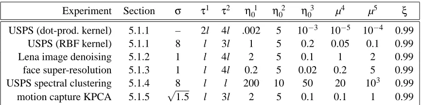
Figure 3: First ten eigenvectors (from left to right) found by KHA/et* for the dot-product (top row)
resp. RBF kernel (bottom row).
5.1.1 USPS DIGITKPCA
Our first benchmark is to perform iterative kernel PCA on a subset of the well-known USPS data set (LeCun et al., 1989)—namely, the first 100 samples of each digit—with two different kernel
functions: the dot-product kernel2
k(x,x0) =x>x0 (39)
and the RBF kernel
k(x,x0) =exp
(x−x0)>(x−x0)
2σ2
(40)
withσ=8, the value used by Mika et al. (1999). We extract the first 16 eigenvectors of the kernel
matrix and plot the excess relative error in Figure 2. Although KHA/et and KHA/et* differ in their transient behavior—the former performing better for the first 6 passes through the data, the latter thereafter—their error after 200 passes is quite similar; both clearly outperform KHA/t. SMD is able
Figure 4: Comparison of excess relative reconstruction error of KHA variants estimating eigenval-ues and updating gains every iteration (’i’) vs. once every pass (’p’) through the USPS data, for RBF kernel PCA extracting 16 eigenvectors.
Figure 5: Lena image—original (left), noisy (center), and denoised by KHA-SMD (right).
to significantly improve the performance of KHA/et but not KHA/et*, and so KHA-SMD achieves the best results on this task. These results hold for either choice of kernel. We show the first 10 eigenvectors obtained by KHA/et* for each kernel in Figure 3.
In Figure 4 we compare the performance of our algorithms, which estimate the eigenvalues and update the gains only once after every pass through the data (’p’), against variants (’i’) which do this after every iteration. Tuning parameters were re-optimized for the new variants, though
most optimal settings remained the same.3 Updating the estimated eigenvalues after every iteration,
Figure 6: Excess relative reconstruction error of KHA variants in our replication of experiments due to Kim et al. (2005). Left: multipatch image kernel PCA on a noisy Lena image; Right: super-resolution of face images.
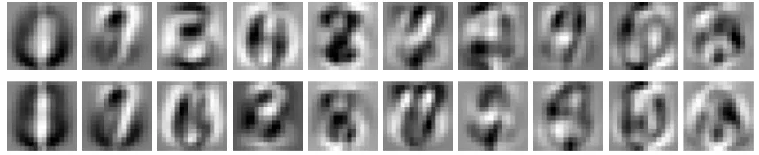
Figure 7: Reconstructed Lena image after (left to right) 1, 2, and 3 passes through the data set, for
KHA with constant gainηt=0.05 (top row) vs. KHA-SMD (bottom row).
5.1.2 MULTIPATCHIMAGEDENOISING
For our second benchmark we replicate the image denoising problem of Kim et al. (2005), the idea being that noise can be removed from images by reconstructing image patches from their r leading
eigenvectors. We divide the well-known Lena image (Munson, 1996) into four sub-images, from
which 11×11 pixel windows are sampled on a grid with two-pixel spacing to produce 3844 vectors
of 121 pixel intensity values each. Following Kim et al. (2005) we use an RBF kernel withσ=1
to find the 20 best eigenvectors for each sub-image. Results averaged over the four sub-images are
plotted in Figure 6 (left), including the KHA with constant gain ofηt=0.05 employed by Kim et al.
(2005) for comparison. The original, noisy, and denoised Lena images are shown in Figure 5. KHA/t, while better than the conventional KHA with constant gain, is clearly not as effective as our methods. Of these, KHA/et is outperformed by KHA/et* but benefits more from the addition of SMD, so that the performance of KHA-SMD is almost comparable to KHA-SMD*. KHA-SMD and KHA-SMD* achieved an excess reconstruction error that is over three orders of magnitude better than the conventional KHA after 50 passes through the data.
Replicating Kim et al.’s (2005) 800 passes through the data with the constant-gain KHA we obtain an excess relative reconstruction error of 5.64%, 500 times that of KHA-SMD after 50 passes.
The signal-to-noise ratio (SNR) of the reconstruction after 800 passes with constant gain is 13.46,4
comparable to the SNR of 13.49 achieved by KHA/et* in 50 passes.
To illustrate the large difference in early performance between conventional KHA and KHA-SMD, we show the images reconstructed from either method after 1, 2, and 3 passes through the data set in Figure 7. KHA-SMD delivers good-quality reconstructions very quickly, while those of the conventional KHA are rather blurred.
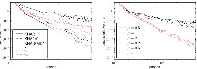
We now investigate how the different components of KHA-SMD* affect its performance. The overall gain used by KHA-SMD* comprises three factors: the scheduled gain decay over time (9), the reciprocal of the current estimated eigenvalues, and the gain adapted by SMD. Let us denote these three factors as t, e, and s, respectively, and explore which of their combinations make sense. We clearly need either t or s to give us some form of gain decay, which e does not provide. This means that in addition to the KHA/t (using only t), KHA/et* (t and e), and KHA-SMD* (t, e, and
s) algorithms, there are three more feasible variants: a) s alone, b) t and s, and c) e and s.
We compare the performance of these “anonymous” variants to that of KHA/t, KHA/et*, and KHA-SMD* on the Lena image denoising problem. Parameters were tuned for each variant
in-dividually, yieldingη0=0.5 and µ=2 for variant s, η0=1 and µ=2 for variant es, andτ=l,
η0=2, and µ=1 for variant ts. Figure 8 (left) shows the excess relative error as a function of
the number of passes through the data. On its own, SMD (s) outperforms the scheduled gain de-cay (t), but combining the two (ts) is better still. Introducing the reciprocal eigenvalues (e) further improves performance in every context. In short, all three factors convey a significant benefit, both individually and in combination. The “anonymous” variants represent intermediate forms between the (poorly performing) KHA/t and KHA-SMD*, which combines all three factors to attain the best results.
Next we examine the sensitivity of the KHA with SMD to the value of the meta-gain µ by
increasing µ∈ {a·10b: a∈ {1,2,5},b∈ {−1,0,1}}until the algorithm diverges. Figure 8 (right)
plots the excess relative error of the s variant (SMD alone, black) and KHA-SMD* (light red) on the Lena image denoising problem for the last three values of µ prior to divergence. In both cases the
largest non-divergent meta-gain (µ=2 for s, µ=1 for KHA-SMD*) yields the fastest convergence.
The differences are comparatively small though, illustrating that SMD is not overly sensitive to the
Figure 8: Excess relative reconstruction error for multipatch image PCA on a noisy Lena image. Left: comparison of original KHA variants (black) with those using other combinations (light red) of gain decay (t), reciprocal eigenvalues (e), and SMD (s). Right: effect of varying µ on the convergence of variant s (black) and KHA-SMD* (light red).
value of µ. This holds in particular for KHA-SMD*, where SMD is assisted by the other two factors,
t and e.
5.1.3 FACEIMAGESUPER-RESOLUTION
We also replicate a face image super-resolution experiment of Kim et al. (2005). Here the eigenvec-tors learned from a training set of high-resolution images are used to predict high-resolution detail from low-resolution test images. The training set consists of 5000 face images of 10 different people
from the Yale face database B (Georghiades et al., 2001), down-sampled to 60×60 pixels. Testing
is done on 10 different images from the same database; the test images are first down-sampled to
20×20 pixels, then scaled back up to 60×60 by mapping each pixel to a 3×3 block of identical
pixel values. These are then projected into a 16-dimensional eigenspace learned from the training
set to predict the test images at the 60×60 pixel resolution.
Figure 6 (right) plots the excess relative reconstruction error of the different algorithms on this task. KHA/t again produces better results than the KHA with constant gain but is ineffective com-pared to our methods. KHA/et* again does better than KHA/et but benefits less from the addition of SMD making SMD-KHA once more the best-performing method. After 50 passes through the data, all our methods achieve an excess reconstruction error about three orders of magnitude better than the conventional KHA, though KHA-SMD is substantially faster than the others at reaching this level of performance. Figure 9 illustrates that the reconstructed face images after one pass through the training data generally show better high-resolution detail for KHA-SMD than for the conventional KHA with constant gain.
5.1.4 SPECTRALCLUSTERING OFUSPS DIGITS
Figure 9: Rows from top to bottom: Original face images (60×60 pixels); sub-sampled images
(20×20 pixels); super-resolution images produced by KHA after one pass through the
1. Define the normalized transition matrix P :=D−12KD− 1
2, where K∈Rl×l is the kernel
matrix of the data, andDis a diagonal matrix with[D]ii=∑j[K]i j.
2. LetA∈Rr×l be the matrix whose rows correspond to the first r eigenvectors ofP.
3. Normalize the columns ofAto unit length, and map each input pattern to its corresponding
column inA.
4. Cluster the columns ofAinto r clusters (using, for instance, k-means clustering), and assign
each pattern to the cluster its corresponding column vector belongs to.
We can obviously employ the KHA in Step 2 above. We evaluate our results in terms of the variation
of information (VI) metric (Meila, 2005): For a clustering algorithm c, let|c|denote the number of
clusters, and c(·)its cluster assignment function, that is, c(xi) = j iff c assigns patternxito cluster
j. Let Pc∈R|c| denote the probability vector whose jth component denotes the fraction of points
assigned to cluster j, and Hcthe entropy associated with Pc:
Hc=− |c|
∑
i=1
[Pc]iln[Pc]i. (41)
Given two clustering algorithms c and c0we define the confusion matrix Pcc0∈R|c|×|c0|by
[Pcc0]km=1
l|{i|(c(xi) =k)∧(c
0(xi) =m)}|, (42)
where l is the number of patterns. The mutual information Icc0 associated with Pcc0 is
Icc0 = |c|
∑
i=1 |c0|
∑
j=1
[Pcc0]i jln [Pc0
c ]i j
[Pc]i[Pc0]j. (43)
The VI metric is now defined as
VI=Hc+Hc0−2Icc0. (44)
Our experimental task consists of applying spectral clustering to all 7291 patterns of the USPS data (LeCun et al., 1989), using 10 kernel principal components. We used a Gaussian kernel with
σ=8 and k-means with k=10 (the number of labels) for clustering the columns of A. The
clusterings obtained by our algorithms are compared to the clustering induced by the class labels. On the USPS data, a VI of 4.54 corresponds to random grouping, while clustering in perfect accordance with the class labels would give a VI of zero.
In Figure 10 (left) we plot the VI metric as a function of the number of passes through the data. All our accelerated KHA variants converge towards an optimal clustering in less than 10 passes—in fact, after around 7 passes their results are statistically indistinguishable from that obtained by using an exact eigensolver (labeled ‘PCA’ in Figure 10, left). KHA/t, by contrast, needs about 30 passes through the data to reach a similar level of performance.
The excess relative reconstruction errors—for spectral clustering, of the matrixP—plotted in
Figure 10: Quality of spectral clustering of the USPS data using an RBF kernel, as measured by variation of information (left) and excess relative reconstruction error (right). Hori-zontal ‘PCA’ line on the left marks the variation of information achieved by an exact eigensolver.
Figure 11: Excess relative reconstruction error on human motion capture data.
5.1.5 HUMANMOTIONDENOISING
For our next experiment we employ the KHA to denoise a human walking motion trajectory from
the CMU motion capture database (http://mocap.cs.cmu.edu), converted to Cartesian
coordi-nates via Neil Lawrence’s matlab motion capture toolbox (http://www.dcs.shef.ac.uk/˜neil/
Figure 12: Reconstruction of human motion capture data: One frame of the original data (left), a superposition of this original and the noisy data (center), and a superposition of the original and reconstructed (i.e., denoised) data (right).
motion is reconstructed inR3 via the KHA with an RBF kernel (σ=√1.5); the resulting excess
relative error is shown for various KHA variants in Figure 11.
As in the previous experiment, KHA/et* clearly outperforms KHA/et which in turn is better than KHA/t. Again SMD is able to improve KHA/et to a much larger extent than KHA/et*, though not enough to surpass the latter. KHA/et* reduces the noise variance by 87.5%; it is hard to visually detect any difference between the denoised frames and the original ones—see Figure 12 for an example.
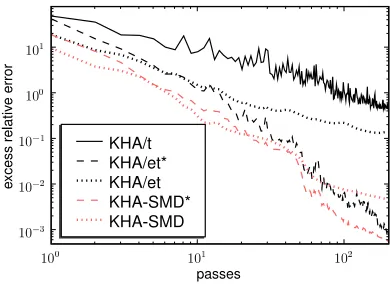
5.2 Experiments on MNIST Data Set
The MNIST data set (LeCun, 1998) consists of 60000 handwritten digits, each 28×28 pixels in
size. While kernel PCA has previously been applied to subsets of this data, to the best of our knowledge nobody has attempted it on the entire data set—for obvious reasons: the full kernel
matrix has 3.6·109entries, requiring over 7 GB of storage in single-precision floating-point format.
Storing this matrix in main memory is already a challenge, let alone computing its eigenvalues; it thus makes sense to resort to iterative schemes.
excess reconstruction error relative to the optimal reconstruction error to measure the performance of the KHA. For MNIST this is no longer possible since existing eigensolvers cannot handle such a large matrix. Instead we simply report the reconstruction error (38), which we can still compute— albeit with a rather high time complexity, as it requires calculating all entries of the kernel matrix.
Since our algorithms are fairly robust with respect to the value ofτ, we simply setτ=0.05l a
priori, which corresponds to decreasing the gain by a factor of 20 during the first (and only) pass
through the data. In our previous experiments we observed that the best values of η0 and µ were
usually the largest ones for which the run did not diverge. We also found that when divergence occurs, it tends to do so early and dramatically, making this event simple and inexpensive to detect.
Algorithm 2 exploits this to automatically tune a gain parameter (η0resp. µ):
Algorithm 2 Auto-tune gain parameter x for KHA (any variant)
1. Compute (Algorithm 1, Step 1) and save initial KHA state;
2. x :=500;
3. While∀i,j : is finite([At]i j):
Run KHA (Algorithm 1, Step 2) for 100 iterations;
4. x :=max
a,b a·10 b: a
∈ {1,2,5},b∈Z,a·10b<x;
5. restore initial KHA state and Goto Step 3.
Algorithm 2 starts with a parameter value so large (here: 500) as to surely cause divergence
(Step 2). It then runs the KHA (any variant) while testing the coefficient matrix At every 100
iterations for signs of divergence (Step 3). If any element ofAt becomes infinite or NaN (“not a
number”), the KHA has diverged; in this case the parameter value is lowered (Step 4) and the KHA restarted (Step 5). In order to make these restarts efficient, we have precomputed and saved in Step
1 the initial state of the KHA—namely a row ofMK, an element ofMKM, the initial coefficient
matrixA1, and A1K0. Once the parameter value is low enough to avoid divergence, Algorithm 2
runs the KHA to completion in Step 3.
We use Algorithm 2 to tune η0 for KHA/et and KHA/et*, and µ for SMD and
KHA-SMD*. Forη0the SMD variants use the same value as their respective non-SMD analogues. In our
experiments, divergence always occurred within the first 600 iterations (1% of the data), or not at all.
It is therefore possible to tune bothη0and µ for the SMD variants as follows: first run Algorithm 2
to tuneη0(with µ=0) on a small fraction of the data, then run it a second time to tune µ (with the
previously obtained value forη0) on the entire data set.
Our experiments were performed on an AMD Athlon 2.4 GHz CPU with 2 GB main memory
and 512 kB cache, using a Python interface to PETSc (http://www-unix.mcs.anl.gov/petsc/
petsc-as/). For a fair comparison, all our algorithms use the same initial random matrix A1,
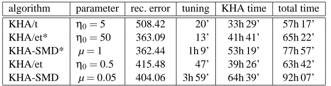
algorithm parameter rec. error tuning KHA time total time
KHA/t η0=5 508.42 20’ 33h 29’ 57h 17’
KHA/et* η0=50 363.09 13’ 41h 41’ 65h 22’
KHA-SMD* µ=1 362.44 1h 9’ 53h 19’ 77h 57’
KHA/et η0=0.5 415.48 47’ 39h 26’ 63h 42’
KHA-SMD µ=0.05 404.06 3h 59’ 64h 39’ 92h 07’
Table 2: Tuned parameter values (col. 2), reconstruction errors (col. 3), and runtimes for various KHA variants on the MNIST data set. The total runtime (col. 6) is the sum of the times required to: center the kernel (11h 13’), tune the parameter (col. 4), run the KHA (col. 5), and calculate the reconstruction error (12h 16’).
Table 2 also reports the time spent in parameter tuning, the resulting tuned parameter values, the time needed by each KHA variant for one pass through the data, and the total runtime (comprising kernel centering, parameter tuning, KHA proper, and computing the reconstruction error). Our KHA variants incur an overhead of 10–60% over the total runtime of KHA/t; the SMD variants are the more expensive. In all cases less than 5% of the total runtime was spent on parameter tuning.
6. Discussion and Conclusion
We modified the kernel Hebbian algorithm (KHA) of Kim et al. (2005) by providing a separate gain for each eigenvector estimate, and presented two methods, KHA/et* and KHA/et, which set those gains inversely proportional to the current estimate of the eigenvalues. KHA/et has a normalization term which allowed us to eliminate one of the free parameters of the gain decay scheme. Both methods were then enhanced by applying stochastic meta-descent (SMD) to perform gain adaptation in RKHS.
We compared our algorithms to the conventional approach of using KHA with constant gain,
resp. with a scheduled gain decay (KHA/t), in seven different experimental settings. All our methods
clearly outperformed the conventional approach in all our experiments. KHA/et* was superior to
KHA/et, at the cost of having an additional free parameter τ. Its parameters, however, proved
particularly easy to tune, withη0=5 andτ=3l or 4l optimal in all but the spectral clustering and
MNIST experiments. This suggests that KHA/et* has good normalization properties and may well be preferable to KHA/et.
SMD improved the performance of both KHA/et and KHA/et*, where the improvements for the former were often larger than for the latter. This is not surprising per se, as it is naturally easier to improve upon a good algorithm than an excellent one. However, the fact that KHA-SMD frequently outperformed KHA-SMD* indicates that the interaction between KHA/et and SMD appears to be more effective.
(e.g., Platt, 1999; Joachims, 1999; Zanni et al., 2006). This is done for kernel PCA by the KHA (Kim et al., 2005), which as originally introduced suffers from slow convergence. The acceleration techniques we have introduced here rectify this situation, and hence open the way for kernel PCA to be applied to large data sets.
Acknowledgments
We would like to thank the anonymous reviewers for their helpful comments. A short version of this paper was presented at the 2006 NIPS conference (Schraudolph et al., 2007). National ICT Australia is funded by the Australian Government’s Department of Communications, Information Technology and the Arts and the Australian Research Council through Backing Australia’s Ability and the ICT Center of Excellence program. This work is supported by the IST Program of the European Community, under the Pascal Network of Excellence, IST-2002-506778. Finally, we would like to acknowledge Equations (8), (10), (11), (12), (15), (21), (27), (28), (39), (40), (41), (42), (43), and (44) here, so that they are numbered.
References
Stephen Boyd and Lieven Vandenberghe. Convex Optimization. Cambridge University Press, Cam-bridge, England, 2004.
Liang-Hwe Chen and Shyang Chang. An adaptive learning algorithm for principal component analysis. IEEE Transaction on Neural Networks, 6(5):1255–1263, 1995.
Christian Darken and John E. Moody. Towards faster stochastic gradient search. In John E. Moody, Stephen J. Hanson, and Richard Lippmann, editors, Advances in Neural Information Processing
Systems, volume 4, pages 1009–1016. Morgan Kaufmann Publishers, 1992.
Athinodoros S. Georghiades, Peter N. Belhumeur, and David J. Kriegman. From few to many: Illumination cone models for face recognition under variable lighting and pose. IEEE
Transac-tions on Pattern Analysis and Machine Intelligence, 23(6):643–660, 2001. ISSN 0162-8828. doi:
http://doi.ieeecomputersociety.org/10.1109/34.927464.
Andreas Griewank. Evaluating Derivatives: Principles and Techniques of Algorithmic
Differentia-tion. Frontiers in Applied Mathematics. SIAM, Philadelphia, 2000.
Thorsten Joachims. Making large-scale SVM learning practical. In Bernhard Sch ¨olkopf, Chris J. C. Burges, and Alex J. Smola, editors, Advances in Kernel Methods — Support Vector Learning, pages 169–184, Cambridge, MA, 1999. MIT Press.
Juha Karhunen. Optimization criteria and nonlinear PCA neural networks. In IEEE World Congress
on Computational Intelligence, volume 2, pages 1241–1246, 1994.
Kwang In Kim, Matthias O. Franz, and Bernhard Sch ¨olkopf. Iterative kernel principal component analysis for image modeling. IEEE Trans. Pattern Analysis and Machine Intelligence, 27(9): 1351–1366, 2005.
Yann LeCun. MNIST handwritten digit database, 1998. URLhttp://www.research.att.com/
˜yann/ocr/mnist/.
Yann LeCun, Bernhard E. Boser, John S. Denker, Donnie Henderson, R. E. Howard, Wayne E. Hubbard, and Lawrence D. Jackel. Backpropagation applied to handwritten zip code recognition.
Neural Computation, 1:541–551, 1989.
Marina Meila. Comparing clusterings: An axiomatic view. In Proc. 22nd Intl. Conf. Machine
Learning (ICML), pages 577–584, New York, NY, USA, 2005. ACM Press.
Sebastian Mika, Bernhard Sch ¨olkopf, Alex J. Smola, Klaus-Robert M ¨uller, Matthias Scholz, and Gunnar R¨atsch. Kernel PCA and de-noising in feature spaces. In Michael S. Kearns, Sara A. Solla, and David A. Cohn, editors, Advances in Neural Information Processing Systems, vol-ume 11, pages 536–542. MIT Press, 1999.
David C. Munson, Jr. A note on Lena. IEEE Trans. Image Processing, 5(1), 1996.
Andrew Y. Ng, Michael I. Jordan, and Yair Weiss. On spectral clustering: Analysis and an algo-rithm. In Thomas G. Dietterich, Suzanna Becker, and Zoubin Ghahramani, editors, Advances in
Neural Information Processing Systems, volume 14, 2002.
Erkki Oja and Juha Karhunen. On stochastic approximation of the eigenvectors and eigenvalues of the expectation of a random matrix. Journal of Mathematical Analysis and Applications, 106(1): 69–84, February 1985.
Barak A. Pearlmutter. Fast exact multiplication by the Hessian. Neural Computation, 6(1):147–160, 1994.
John Platt. Fast training of support vector machines using sequential minimal optimization. In Bernhard Sch ¨olkopf, Chris J. C. Burges, and Alex J. Smola, editors, Advances in Kernel
Meth-ods — Support Vector Learning, pages 185–208, Cambridge, MA, 1999. MIT Press.
Herbert Robbins and Sutton Monro. A stochastic approximation method. Annals of Mathematical
Statistics, 22:400–407, 1951.
Terrence D. Sanger. Optimal unsupervised learning in a single-layer linear feedforward network.
Neural Networks, 2:459–473, 1989.
Bernhard Sch ¨olkopf and Alex J. Smola. Learning with Kernels. MIT Press, Cambridge, MA, 2002.
Bernhard Sch ¨olkopf, Alex J. Smola, and Klaus-Robert M ¨uller. Nonlinear component analysis as a kernel eigenvalue problem. Neural Computation, 10:1299–1319, 1998.
Nicol N. Schraudolph. Fast curvature matrix-vector products for second-order gradient descent.
Nicol N. Schraudolph. Local gain adaptation in stochastic gradient descent. In Proc. Intl. Conf.
Artificial Neural Networks, pages 569–574, Edinburgh, Scotland, 1999. IEE, London.
Nicol N. Schraudolph, Simon G ¨unter, and S. V. N. Vishwanathan. Fast iterative kernel PCA. In Bernhard Sch ¨olkopf, John Platt, and Thomas Hofmann, editors, Advances in Neural Information
Processing Systems, volume 19, Cambridge MA, June 2007. MIT Press.
Therdsak Tangkuampien and David Suter. Human motion de-noising via greedy kernel principal component analysis filtering. In Proc. Intl. Conf. Pattern Recognition, 2006.
S. V. N. Vishwanathan, Nicol N. Schraudolph, and Alex J. Smola. Step size adaptation in reproduc-ing kernel Hilbert space. Journal of Machine Learnreproduc-ing Research, 7:1107–1133, June 2006.