Int. J. Industrial Mathematics Vol. 1, No. 1 (2009) 13-18
Determining the Best Performance Time Period
of a System
A. Dehnokhalajia, N. Nasrabadia, N.A. Kianib
(a) Department of Mathematical Sciences, Tehran Teacher Training University, Tehran, Iran. (b) Department of Mathematics, Science and Research Branch, Islamic Azad University, Tehran, Iran.
||||||||||||||||||||||||||||||||{ Abstract
The main purpose of this paper is to determine the best performance time period of a system, consisting some DMUs, among some sequential time periods. This aim is satised by two proposed algorithms, the rst based on global Malmquist Productivity Index and the second is based on PPS frontiers.
Keywords: DEA, Best Performance Time Period, Global Malmquist Productivity Index.
||||||||||||||||||||||||||||||||||
1 Introduction
Data Envelopment Analysis, which was suggested by Charnes, Cooper and Rhodes (CCR[1]) and built on the idea of Farrell, is a well-known OR technique for assessing the relative eciency of a set of similar and comparable decision making units. Based on CCR model, several extension of DEA models have been introduced that depend on the technology and circumstances any of them can be used to evaluate the relative eciency of each DMU in the system at a pre-determined time period. But in some situations, the problem of comparing the productivity of a DMU between two time period arises. In this regard, we need a bilateral index for measuring the productivity changes. Toward this end, one of the most popular approaches is based on using Malmquist Productivity Index, a method originated by Caves et al.[2]. Malmquist Productivity Index that is in the form of ge-ometric mean, can be decomposed into two components namely eciency changes and technological changes. Malmquist Productivity Index is a tool provide us to compare the productivity of a DMU between two time period[6], but in some cases we need to compare the productivity of the hole system at two time period. The general case is that when we are interested in the performance of the system in T time periods(T 2). For example
we want to determine the Best Performance Time Period(BPTP), by BPTP we mean the period in which the system has performed best. In this paper we provide two approaches for determining the BPTP.
The paper is organized as follows. Sec. 2 provides some preliminaries and basic denitions. Sec. 3 presents two approaches for determining the BPTP. Finally, a numerical example is brought in Sec. 4.
2 Preliminaries
Consider a set of n DMUs S = fDMU1; : : : ; DMUng and suppose that we are interested
in the performance of this system at any time period t, t 2 T = f1; : : : ; T g. Assume that at time period t, each DMUj uses the vector of inputs Xjt= [xt1j; : : : ; xtmj] 2 <m to
produce the vector of outputs Yt
j = [y1jt ; : : : ; ytsj] 2 <s.
Denition 2.1. For each t 2 T , the production possibility set at time period t is dened as:
Pt= f(Xt; Yt)j at time period t; Xt can produce Ytg: Denition 2.2. The global production possibility set is dened as:
PG= conv(
T
[
t=1
Pt):
Lemma 2.1. If for each t 2 T , Ptsatises in axioms constant return to scale & convexity
and all inputs & outputs are freely disposable and all observations belong to PG, then PG
will also satisfy in all 4 axioms and it will be represented as:
PG= f(X; Y )jX XT t=1
n
X
j=1
t
jXjt; Y T
X
t=1 n
X
j=1
t
jYjt; tj 0; t = 1; : : : ; T; j = 1; : : : ; ng
Denition 2.3. The distance function for DMUo at time period t with respect to Pt0 is
dened as:
Dt0
(DMUt
o) = Dt0(Xot; Yot) = inffj(Xot;Y t o
) 2 Pt
0
g:
Denition 2.4. The distance function for DMUo at time period t with respect to PG is
dened as:
DG(DMUot) = DG(Xot; Yot) = inffj(Xot;Yot) 2 PGg:
Corollary 2.1. For every o 2 f1; : : : ; ng and every ^t2 T , we have:
DG(Xo^t; Yo^t) minfDt(Xo^t; Yo^t)jt = 1; : : : ; T g
Corollary 2.2. For each o 2 f1; : : : ; ng and each t 2 f1; : : : ; T g, DG(Xt
Consider an arbitrary DMUo 2 S and two time periods t1; t2 2 T ,(t1 < t2). To
compare the productivity of DMUo at time period t2 with its productivity at time period
t1, we can use contemporary Malmquist productivity index, Mc, which is a bilateral index:
Mc
o(t1; t2) =
Dt1(Xt2
o ; Yot2)
Dt1(Xot1; Yot1)
Dt2(Xt2
o ; Yot2)
Dt2(Xot1; Yot1)
1 2
Mc
o(t1; t2) > 1(< 1), indicates that the productivity of DMUo at time period t2 is
bet-ter(worse) than its productivity at time period t1.
It is shown that Mc is not a circular index[4]. So, a new index MG, was provided which
satises in the circulatory test[5].
Denition 2.5. A global Malmquist productivity index is dened as:
MG
o (t1; t2) = D G(Xt2
o ; Yot2)
DG(Xt1
o ; Yot1)
MG
o (t1; t2) > 1(< 1), indicates that the productivity of DMUo at time period t2 is
better(worse) than its productivity at time period t1.
In comparison with contemporary Malmquist Productivity Index (Mc), MG has some
desirable properties that are omitted here[5].
3 The Best Performance Time Period
In some situations, it is important to have some information about the total performance of system S at a given time period t.
In this section we will provide two measures for determining the best performance time period(BPTP) among T time periods 1; : : : ; T . Toward this end, we bring the following denition.
Denition 3.1. For each t 2 T , the vector of eciency at time period t is dened as:
t= [DG(X1t; Y1t); : : : ; DG(Xnt; Ynt)]
Assume that E = f1; : : : ; Tg. It is obvious that if t is the BPTP, then t
would be a non-dominated vector in E. Therefore, to determine the BPTP we will focus only on time periods that their eciency vectors are non-dominated in E. Given ^t2 T , we apply the following model to determine whether ^tis non-dominated or not.
^t= max d
s:t: P^t+ d PTt=1tt T
t=1t= 1
t2 f0; 1g t = 1; : : : ; T
(1)
Theorem 3.1. ^tis non-dominated in E if and only if ^t= 0.
3.1 A Method Based on MG
In this method we will use the concept of MG to provide a measure which determines the
BPTP. As mentioned before, we will focus only on non-dominated elements of E. Let IE
be a subset of T consisting the indices of all non-dominated elements in E. Associated with each t 2 IE we dene a n-dimensional vector t= [t1; : : : ; tn] where tj = MjG(1; t),
for j = 1; : : : ; n.
Therefore, for each t 2 IE, t is a vector that its jth entry identies progress or regress
of DMUj between two time periods 1 and t.
Remember that our goal is to determine a time period t among 1; : : : ; T in which the
hole system S has performed best. In this regard, we can consider tas a criterion. As a
fact, t is a vector that represents the total progress or regress of system S between time
period 1 and t. It means that the bigger entries of t, the more productivity of system S
at time period t in comparison with the rst time period. So if t is the BPTP, then t
should be non-dominated in ftjt 2 I Eg.
Lemma 3.1. Let t = Pn
j=1tj
n for each t 2 IE and assume that t = maxftjt 2 IEg.
Then t
is non-dominated in ftjt 2 I Eg.
Based on the above lemma, the following algorithm is proposed for BPTP.
Algorithm 1
Step1. Form the set IE by applying model (1).
Step2. For each t 2 IE calculate t= Pn
j=1tj
n .
Step3. The time period t where
t = maxftjt 2 IEg is the BPTP.
3.2 Method Based on Technology Changes
In the following method, the dierence between the boundary of two production possibility sets is used as a criterion for determining the BPTP. We can say that the more similarity between the boundaries of PG and Pt indicates the better performance of system S at
time period t. So, rst we provide a tool which measures the dierences between two boundary. Toward this end, associated with each t 2 IE we dene a n-dimensional vector
t= [t
1; : : : ; nt] where jt= D
G(Xt j;Yjt)
Dt(Xt
j;Yjt), j = 1; : : : ; n.
Now we can observe that t
j shows the dierence between the boundary of PG and Pt
along the ray f(Xt
j; Yjt))j 0g.
Let t = Pn
j=1tj
n for each t 2 IE. Note that t 1 for each t. The bigger amount of
t indicates the more similarity between the two production possibility sets PG and Pt.
Therefore t is the desirable criterion in determining the BPTP and the proposed
algo-rithm is as follows:
Algorithm 2
Step1. Form the set IE by applying model (1).
Step2. For each t 2 IE calculate t= Pn
j=1tj
Step3. The time period t where
t = maxftjt 2 IEg is the BPTP.
4 Numerical Example
In order to illustrate the proposed methods, we bring an example. The system under evaluation consists six DMUs, each DMU uses 2 inputs to produce 2 outputs. We have considered this system in 4 time periods. The problem is to determine the BPTP of the system among 4 time periods. The data of the system and DMU's eciency scores at each time period are given in Table 1.
t 1 2 3 4
DMU1 0.009 0.743 0.154 0.544
DMU2 0.106 0.207 0.154 0.371
DMU3 1.000 1.000 1.000 1.000
DMU4 0.457 0.756 0.391 0.490
DMU5 0.151 0.163 0.160 0.356
DMU6 1.000 0.430 1.000 1.000
Table 1. DMUs's eciency
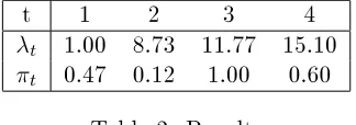
We have applied both Algorithm 1 and Algorithm 2 to nd the BPTP. The results are shown in Table 2.
t 1 2 3 4
t 1.00 8.73 11.77 15.10
t 0.47 0.12 1.00 0.60
Table 2. Results
We observe that Algorithm 1 gives t = 4 as the BPTP, whereas Algorithm 2 gives
t = 3 as the BPTP. This dierence is occurred because of the basic concept of two
algorithms, Algorithm 1 uses the progress (or regress) of the system as a criterion and Algorithm 2 determine the BPTP via measuring the dierence between the frontier of the global production possibility set and the contemporary production possibility set.
5 Conclusion
References
[1] A. Charnes, W.W. Cooper, E. Rhodes, Measuring the eciency of decision making units, European Journal of Operational Research 2(1978), 429{444.
[2] D.W. Caves, L.R. Christensen, E.W. Diewert, The economic theory of index numbers and the measurement of input output, and productivity, Econometrica 50(1982), 1393{ 1414.
[3] R. Fare, S. Grosskopf, B. Lindgren, P. Roos, "Productivity Developments in Swedish Hospitals: a Malmquist output index approach", in A. Charnes, W.W. Cooper, A.Y. Lewin, L.M. Seiford(Eds.), Data Envelopment Analysis: Theory, methodology and applications, Kluwer Academic Publishers, 253{272.
[4] F. R. Forsund, On the circularity of the Malmquist Productivity Index, Working paper, 2002.
[5] J. T. Pastor, C. A. K. Lovell, A global Malmquist Productivity Index, economics letters 88(2005), 266-271.