Smart water demand forecasting: Learning from the data
Maria Xenochristou1, Zoran Kapelan1, Chris Hutton2, Jan Hofman3
1 Centre for Water Systems, University of Exeter, North Park Road, Exeter EX4 4QF, UK
2 Wessex Water, Claverton Down Road, Bath BA2 7WW, UK
3 Water Innovation and Research Centre, University of Bath, BA2 7AY Bath Avon, UK
Corresponding author: [email protected]
Abstract
Accurate forecasts of demand are essential for water utilities in order to manage, plan, and optimize the operation of their network. This work aims to develop a new method for short-term water demand forecasting by utilizing a new data-driven approach based on Random Forests, as well as consumption recordings, household, and socio-economic characteristics, and weather data. Initial results, obtained on real-life consumption data from the UK, demonstrate the potential of this method and show the importance of disaggregating consumption when attempting to determine the influence of weather on water demand. In this study, adding weather input to the model achieved improved forecasting accuracy, especially for the aggregation of properties with medium occupancy and affluent residents during summer months.
Keywords: demand forecasting,machine learning, Random Forests, water management
1
Introduction
Predictions of urban water consumption are essential in water economies, especially under the threat of unprecedented water shortages [1]. Short-term water demand forecasting provides estimates of demand over the next hours or weeks to make informed operational, tactical, and strategic decisions that will improve the performance of the network [4, 10].
However, predicting demand is a challenging task, due to its dynamic nature and inherent randomness, as well as the underlying relationships between consumption and multiple other household, socio-economic, and climatological factors that are not yet fully understood. The majority of short-term forecasting models use past consumption over the past week, month, or year as the main predictor, although some studies have
Volume 3, 2018, Pages 2351–2358
considered the effect of climatic variables such as temperature, humidity, and precipitation [10, 12].
A variety of studies have explored the application of machine learning methods such as Artificial Neural Networks, Support Vector Machines, and fuzzy logic in short-term water demand forecasting [6, 7, 8, 12, 18], or even hybrid models that combine one or more methods, but Random Forests have rarely been used in the water demand literature. The few studies that attempted this [1, 2, 10], although limited by data availability, demonstrated the potential of this method to accurately capture the dynamic nature of water consumption.
In addition to this, very little research so far has examined the water use at multi-house or census tract level [4, 9]. Most studies that investigated the effect of weather on water demand [3, 9, 12], did not account for the variability of individual characteristics between households, but instead applied the methodology at large spatial (DMA level), or temporal (monthly) scales.
The current work aims to utilise a very extensive dataset of consumption records, customer characteristics, household data and weather variables in order to enhance the understanding of the weather influence on water demand and use it to provide accurate forecasts of demand at the census tract level.
2
Consumption Data
The current study is based on the Southwest of England (Dorset, Somerset, Wiltshire, and Hampshire). The available data consists of consumption records derived from smart demand meters, available at 15-30 minute intervals from October 2014 to September 2017. The data is available at household level for almost 2,000 properties. In addition to this, a variety of property (garden size, rateable value, metering status) and customer characteristics (ACORN groups, occupancy rates) are also available for most of the households in the dataset.
ACORN is a geodemographic segmentation of the UK’s population based on social factors and population behaviour and it is used to provide an understanding of the different types of people [17]. According to this, consumer groups A, B, and C are classified as “Affluent Achievers”, and groups D and E as “Rising Prosperity”. All groups A to E are classified as “Affluent” in the following. Groups F to J are classified as “Comfortable Communities” in the same guide, whereas groups K to Q are “Financially Stretched”.
The above variables (garden size, rateable value, metering status, ACORN group, and occupancy rate) can be used to segment the households into groups with uniform characteristics that are expected to show a similar sensitivity of water consumption to weather changes.
Lastly, weather data collected at hourly to daily intervals for the same time-period (October 2014 – September 2017) for various weather stations across the Southwest (Avon, Somerset, Gloucestershire, Wiltshire, Dorset, Hampshire) was acquired from the Met office (UK). These datasets are part of the Met Office Integrated Data Archive System (MIDAS) Land and Marine Surface Stations Data that has been recorded from 1853 to present. The following weather variables acquired from various datasets in the MIDAS database were included in the analysis:
Sunshine duration: This corresponds to the total sunshine hours over a 24-hour period, as recorded by a Campbell-Stokes recorder. Where data is not available, the World meteorological organization (WMO) sunshine duration is used instead [15].
Radiation: This is the total radiation amount that comes directly from the sun but not from the rest of the sky. It’s measured in Kjoules per square meter over a 24 hour period [13].
Rainfall: It describes the rainfall accumulation and precipitation over the 24 hour period, recorded using rain gauges at weather stations across the UK [16].
Humidity: This is the mean humidity value over the 24 hour period, derived from humidity sensors [14].
Air temperature: Mean air temperature recorded from 00.00 till 24.00 hours [15].
3
Demand Forecasting Methodology
3.1 Random ForestsRandom Forests are data driven models that consist of an ensemble of decision trees that can be used for classification or regression. At each split of a tree within a forest, a test is performed by selecting a random subset of the independent variables [2]. The explanatory variables that are used as input to the model represent the roots and the output is the leaves [1]. The number of trees to grow and the number of the independent variables to be randomly selected at each node are defined by the user.
frame for operational purposes, the forecasting horizon for this study was chosen to be 1 to 7 days in the future and 7 days of past consumption are used as input data.
3.2 Explanatory variables
Historical time series of consumption have proven to be the most important determining factor in short-term demand forecasting. Past consumption is imported in all models following a sliding window strategy, where the window has a fixed length of 7 days, meaning that when new data is added (next day), old data is removed (7th day in the past) [2]. These 7 values reflect average daily consumptions among all the properties that are included in the corresponding segmentation of data.
Next, additional explanatory factors are added to each model in an attempt to improve forecasting accuracy. These factors are mainly representative of a variety of weather variables such as air temperature, rainfall, humidity, and sunshine hours, as well as temporal characteristics, i.e. season and type of day (working day or holiday).
Previous qualitative studies [5] concluded that certain types of households (e.g. affluent residents and medium occupancy households) show a higher sensitivity to weather changes during certain times (e.g. weekdays, evenings, and summers), with regards to consumption. The current study attempts to test this conclusion using a quantitative analysis, based on Random Forests. For that purpose, the influence of several weather variables on water consumption is tested and demonstrated for two aggregations of data, one including all the properties and days in the data, and the other one including only consumption during the summer months, households with medium occupancy (2 to 3 people) and affluent residents, as their consumption is expected to be more sensitive to weather changes [5].
Nine model configurations were developed in order to compare the individual as well as combined effect of different variables on the forecasting accuracy, for the two segmentations of properties (Table 1).
The first model accounts only for past consumption, models 2 to 7 account for past consumption as well as one weather variable, whereas models 8 and 9 combine multiple variables and were the two configurations that produced the best results in this study (Table 1).
For each model testing, the available data was divided into two sets, a calibration dataset (80%) used to train the model and a validation dataset (20%) used to test the model performance on unseen data.
3.3 Performance indices
Two performance metrics were used in order to assess the quality of the models’ predictions, the Mean Absolute Error (MAE) and the coefficient of determination (R2);
n
i yi ypre
n MAE 1 1 (1)
2 2 2 y y y y R i pre (2)where yi and ypre are the observed and forecasted values, respectively, and 𝑦̅ is the
mean value of the observed values.
4
Results and discussion
The forecasting accuracy of the 9 models is compared against two datasets, based on the MAE and R2, for different forecast horizons (1 to 7 days ahead). A summary of the results, based on the validation dataset, appears in Figures 1 and 2.
Figure 1 demonstrates the MAE of forecasts for the 9 models. The graph on the left was created based on data for all the properties and days (1,689 households, 1,019 days), whereas the graph on the right takes into account only properties with medium occupancy and affluent residents (166 households) during summer months (297 days in total), as this segmentation of consumption proved to be significantly affected by changes in the weather.
6%) (Figure 1, left graph, model 9). On the other hand, when looking at the properties and time of the year when the weather has the strongest influence on consumption (Figure 1, right graph), accounting for the above weather variables can reduce the error by up to 44%, taking the MAE from ~25 l/property/day to ~14 l/property/day for forecasts 7 days ahead (Figure 1, right graph, model 9). When looking only at summer months and medium occupancy households, humidity alone reduces the error by 24% (25 to 19 l/property/day) (Figure 1, right graph, model 7).
The improvement in performance becomes larger as the forecast horizon grows. Although it is relatively easier to predict water demand for one day ahead (max absolute error improvement is 33%, from ~12 to ~18 l/property/day) (Figure 1, right graph, model 9), accounting for explanatory factors becomes more important the further the prediction moves into the future, resulting in reducing the error by an additional 11% for forecasts 7 days ahead (Figure 1, right graph, model 9).
When attempting short-term forecasts of a few hours or days ahead, information relating to the weather is incorporated in the information about past consumption, as in the UK there are not typically rapid changes in the weather from one day to the next one. However, as the forecast horizon increases, information about the weather becomes valuable when attempting to predict demand, especially when water is used for outdoor activities (recreational and gardening) that primarily happen during the summer months, in affluent households. In addition, segmenting properties with medium occupancy ensure that this correlation can be identified and the relationship between water consumption and demand is not going to be concealed by the erratic water use of single-person households, or even large families.
Figure 1: Mean Absolute Error (MAE) for 1-7 day forecasts, based on the validation dataset, for all properties in all months (left) and for the properties with medium occupancy
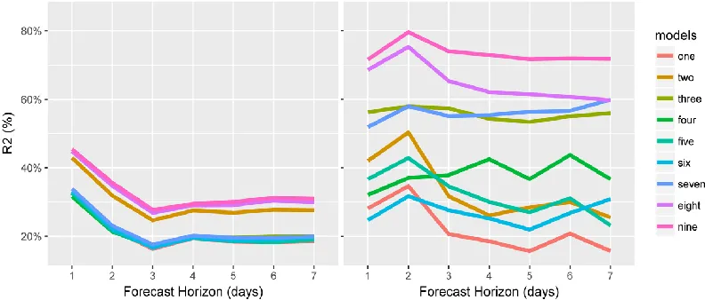
Figure 2 shows the R2 values for the 1-7 day forecasts made by the 9 models. For all properties and days in the data, including weather input increases the value of the R2
from ~20% to ~30% for forecasts 7 days ahead, i.e. by a maximum of just over 10% (Figure 2, left graph), which remains relatively stable over the forecasting horizon. However, adding weather inputs for the properties that are more influenced by the weather variations can increase the R2 values from ~30% to ~72% for forecasts 1 day ahead, or from ~16% to ~72% for forecasts 7 days ahead (Figure 2, right graph). This corresponds to an improvement in correlation of 40% and 56% for forecasts 1 and 7 days ahead, respectively.
5
Conclusions
This study attempts to investigate the influence of multiple weather variables on water consumption by developing a new modelling approach based on Random Forests. Results show that the benefit of adding weather input to demand forecasting models is not univariate across all properties and times of the year but for households with high weather induced consumption it can be significant.
Results obtained also demonstrate the additional value of weather input as the forecast horizon increases, even in the moderate UK climate. When looking at summer months and properties with medium occupancy and affluent residents, adding weather input achieved a reduction of the MAE by up to 44% for forecasts 7 days ahead and an increase of the R2 value by ~56%, as opposed to 20% and 40% respectively for the case where all properties in all months were considered.
Figure 2: Coefficient of determination (R2) for 1-7 days forecasts, based on the validation dataset, for all properties in all months (left) and for the properties with medium
Acknowledgements
This study was conducted as part of the WISE Centre for Doctoral Training, funded by the UK Engineering and Physical Sciences Research Council.
References
[1] G. Chen, T. Long, J. Xiong, Y. Bai, Multiple Random Forests Modelling for Urban Water Consumption Forecasting, J. Water Resources Management 31 (2017) 4715-4279.
[2] M. Herrera, L. Torgo, J. Izquierdo, R. Perez-Garcia, Predictive models for forecasting hourly urban water demand, J. Hydrology, 387 (2010) 141-150.
[3] M. Bakker, H. van Duist, K. Van Schagen, J. Vreeburg, L. Rietveld, Improving the performance of water demand forecasting models by using weather input, Procedia Engineering, 70 (2014) 93-102. [4] A.S. Polebitski, R.N. Palmer, Seasonal Residential Water Demand Forecasting for Census Tracts,
J. Water Resources Planning & Management, 136 (2010) 27-36.
[5] M. Xenochristou, Z. Kapelan, C.J. Hutton, J. Hofman, Identifying relationships between weather variables and domestic water consumption using smart metering, CCWI (2017) Sheffield.
[6] C. Pena-Guzman, J. Melgarejo, D. Prats, Forecasting Water Demand in Residential, Commercial, and Industrial Zones in Bogota, Colombia, Using Least-Squares Support Vector Machines, J. Mathematical Problems in Engineering (2016).
[7] A. Candelieri, D. Soldi, F. Archetti, Short-term forecasting of hourly water consumption by using automatic metering readers data, Procedia Engineering 119 (2015) 844-853.
[8] M. Romano, Z. Kapelan, Adaptive water demand forecasting for near real-time management of smart water distribution systems, J. Environmental modelling & Software 60 (2014) 265-276. [9] A. S. Polebitski, R.N. Palmer, Seasonal Residential Water Demand Forecasting for Census Tracts,
J. Water Resources Planning Management 136 (2010).
[10] E. Pacchin, S. Alvisi, M. Franchini, A short-term water demand forecasting mdoel using a moving window on previously observed data, Water 172 (2017).
[11] P. Bachari, D. Nekipelov, S.P. Ryan, M. Yang, Machine learning methods for demand estimation, American Economic Review 105 (2015) 481-485.
[12] C.C. Dos Santos, A.J. Pereira Filho, Water Demand Forecasting Model for the Metropolitan Area of Sao
Paulo, Brazil, Water Resources Management, 28 (2014) 4401–4414.
[13] Met Office, MIDAS: Global Radiation Observations. NCAS British Atmospheric Data Centre, 07.03.2018. http://catalogue.ceda.ac.uk/uuid/b4c028814a666a651f52f2b37a97c7c7 (2006).
[14] Met Office, MIDAS: UK Hourly Weather Observation Data. NCAS British Atmospheric Data Centre, 07.03.2018. http://catalogue.ceda.ac.uk/uuid/916ac4bbc46f7685ae9a5e10451bae7c (2006).
[15] Met Office, MIDAS: UK Daily Weather Observation Data. NCAS British Atmospheric Data Centre, 07.03.2018. http://catalogue.ceda.ac.uk/uuid/954d743d1c07d1dd034c131935db54e0 (2006).
[16] Met Office, MIDAS: UK Daily Rainfall Data. NCAS British Atmospheric Data
Centre, 07.03.2018. http://catalogue.ceda.ac.uk/uuid/c732716511d3442f05cdeccbe99b8f90 (2006).
[17] CACI Limited, The ACORN user guide, London, 2014.