Statistical analysis of long-duration low-density solar wind events

Received: 3 July 2000 – Revised: 28 November 2000 – Accepted: 5 December 2000

Abstract. Low solar wind density with long duration was

measured by in situ observation between 11 and 12 May 1999. As a result of this low-density solar wind condition, the magnetosphere of the Earth expanded considerably. We used a database of one-hour-averaged solar wind (1963– 1999) near 1 AU to determine whether or not the observed low-density event was extremely abnormal. As a result it was found that this event has the longest duration in approx-imately 36 years of solar wind observations.

There are three events with density 0.5 cm−3or less and duration ten hours or longer. They were observed on 4 and 31 July 1979, and 11–12 May 1999. The 4 July 1979 event recurred on 31 July 1979. The events were characterized by low-beta, low Alfven Mach number (MA), and low dynamic

pressure. The occurrence rate of low-density solar wind with density 0.5 cm−3or less shows several peaks near solar max-ima. However, it is difficult to find a clear relationship be-tween the sunspot number and the occurrence rate.

Key words. Interplanetary physics (flare and stream

dynam-ics; solar wind plasma; sources of the solar wind)

1 Introduction

Long-duration low-density solar wind was observed between 11 and 12 May 1999. The balance between the magnetic pressure of the geomagnetic field and the dynamic pressure of the solar winds determines the size of the Earth’s magneto-sphere (Fairfield, 1971; Sibeck et al., 1991). The low-density solar winds cause a large expansion of the magnetosphere and the large outward excursion of the Earth’s bow shock (Fairfield, 1971; Cairns et al., 1995; Takeuchi et al., 1998).

The solar wind conditions near 1 AU have been measured since the early 1960s. However, this kind of long-duration low-density solar wind has not been fully studied. We studied historical low-density solar wind events using a large data set to better understand the event that occurred in May 1999. Correspondence to: S. Watari ([email protected]

2 Data sources

We used the one-hour-averaged solar wind parameters (den-sity, speed, temperature, and magnetic field) collected be-tween 1963 and 1999, compiled in the OMNI database. The solar wind data collected by the ACE spacecraft was used for the analysis of the events on 26–27 April 1999, 11–12 May 1999, and 28–30 June 1999.

Figure 1 shows the data coverage of the solar wind density observation for the OMNI database. Continuous solar wind observations by the WIND satellite, augmenting those of the IMP-8 satellite, have increased the coverage since 1995. An earlier period of good coverage was between 1973 and 1982. In this period, the ISSE-3 spacecraft measured solar wind continuously at the L1 point. Between 1983 and 1994, the solar wind near 1 AU was mainly measured using the IMP-8 satellite, and the averaged coverage was approximately 35%. Figure 2 shows the durations of low-density solar wind events (density 0.5 cm−3 or less). We consider solar wind density 0.5 cm−3 or less as “low-density” here. The May 1999 event is the longest low-density solar wind event stud-ied. It lasted 22 hours. The second longest event occurred on 31 July 1979 and lasted 20 hours. The third longest event occurred on 4 July 1979 and lasted ten hours. The aver-aged duration of all low-density events was approximately four hours. Roughly half of the events lasted less than two hours.

num-Fig. 1. Data coverage of solar wind density observations for OMNI data between 1963 and 1999.

Fig. 2. A histogram of duration of low solar wind density events with density 0.5 cm−3or less.

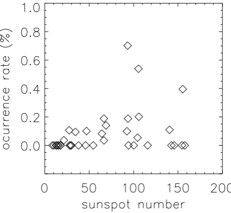
bers and annual occurrence rates of low-density solar wind. According to Fig. 4, it is difficult to find a clear relation-ship between sunspot numbers and occurrence rates of low-density solar wind.

Figure 5 shows scatter plots of density (N) vs. speed (V), N vs. temperature (T),N vs. magnetic field intensity (|B|), N vs. plasma beta (β),N vs. dynamic pressure (Pdyn), and square of speed (V2) vs. Pdyn. We calculatedPdyn by the following equations:Pdyn=mpN V2; wherempis the mass

of proton. We used one-hour-averaged values between 1963 and 1999 to make Fig. 5, where the density varied between 0.1 and 100 cm−3, while the solar wind speed varied between 100 and 1000 km/s. The correlation coefficient between den-sity and dynamic pressure, 0.73 is better than the coefficient betweenV2 andPdyn, 0.23. This suggests that the density is an important factor affecting the dynamic pressure of the Earth’s magnetosphere. The correlation coefficients ofNvs. V,N vs. T,N vs. |B|, andN vs. plasma beta are−0.35, −0.16, 0.23, and 0.08, respectively.

Fig. 3. Yearly sunspot numbers and annual occurrence rates of low-density solar wind (low-density 0.5 cm−3or less).

Fig. 4. A scatter plot of yearly sunspot numbers and annual occur-rence rates of low-density solar wind (density 0.5 cm−3or less).

Cairns et al. (1995) noted that Mach number is important for determining the shape and location of the Earth’s bow shock and that solar wind with low Mach numbers causes large excursion of the Earth’s bow shock. Figure 6 shows scatter plots ofNvs. Alfven Mach number (MA),V vs.MA,

T vs. MA, and|B|vs. MA. The correlation coefficients of

Nvs.MA,V vs.MA,T vs.MA, and|B|vs.MAwere 0.26,

−0.04,−0.10, and−0.50, respectively. SmallerMAtends to

be observed in lower solar wind density as shown in Fig. 6.

3 Historical events of low-density solar wind

Fig. 6. Scatter plots of density (N) and Alfven Mach number (MA), speed (V) vs. MA, temperature (T) vs. MA, and magnetic intensity (|B|) vs.MA.

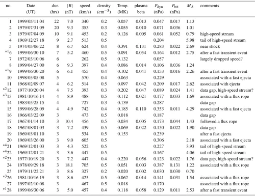
typical values of density, speed, temperature, magnitude of magnetic field, beta, dynamic pressure, total pressure, and MA near 1 AU are 6.6 cm−3, 450 km/s, 0.12 MK, 7 nT,

0.56, 2.23 nPa, 0.049 nPa, and 7.57, respectively. Table 1 shows the dates and durations of the events and the av-eraged solar wind parameters (magnetic intensities, speeds, densities, temperatures, plasma beta, dynamic pressures, to-tal pressures, and MA). We calculated the total pressures

(Ptot) according to the following equations: Ptot = Pgas+ Pmag,Pgas = N k(Tp+Te),Pmag = B2/2µ0; wherePgas, Pmag,k,Tp,Te,B, andµ0are the gas pressure of solar wind, the magnetic pressure of solar wind, the Boltzmann constant, the proton temperature, the electron temperature, the mag-netic field intensity, and the permeability of free space, re-spectively. We assumed that the electron density was equal to the proton density and that theTewas 141 000 K and was

constant (Newbury et al., 1998; Kawano et al, 2000). The low-density solar wind events in Table 1 are characterized by low values of beta, dynamic pressure, andMA.

Approxi-mately 20% of the low-density events in Table 1 were associ-ated with high-speed streams and approximately half of the events were associated with transient solar wind structures (e.g., flux rope, ejecta, and shock). The events associated with flux ropes were approximately 20% in Table 1. High magnetic pressure inside flux ropes is a possible explanation for the low-density events. Several events (e.g., 1 and 27 December 1969, 4 and 31 July 1979) showed recurrent activ-ities. The events on 1 and 27 December 1969 were observed in the tail of high-speed streams.

10 1998/05/05 08 5 570 0.4 0.063 0.229 associated with a fast ejecta 11 1968/02/09 07 4 6.2 514 0.5 0.097 0.042 0.209 0.017 2.62 associated with ejecta

∗2_{12 1977/10/20 04 4 7.5 393 0.3 0.202 0.047 0.089 0.024 1.41 data gap, high-speed stream?}

∗3_{13 1981/10/16 14 4 8.9 488 0.5 0.112 0.021 0.177 0.033 1.69 associated with a flux rope}

14 1983/05/25 15 4 727 0.3 0.139 0.287 data gap

15 1999/06/28 09 4 4.9 742 0.4 0.185 0.110 0.353 0.011 4.29 associated with a fast ejecta

16 1966/03/22 09 3 473 0.5 0.018 0.187 data gap

17 1967/01/14 10 3 10.4 456 0.5 0.034 0.005 0.173 0.044 1.43 followed a flux rope 18 1967/08/01 03 3 7.2 439 0.5 0.069 0.022 0.150 0.022 1.90 data gap

19 1969/03/01 10 3 534 0.5 0.153 0.239 after a fast ejecta

20 1969/03/26 00 3 9.0 605 0.5 0.306 2.18 associated with a fast ejecta

∗4_{21 1969/12/01 03 3 4.3 522 0.5 0.227 3.93 tail of high-speed stream}

∗4_{22 1969/12/01 21 3 3.6 447 0.5 0.167 4.06 tail of high-speed stream}

∗2_{23 1977/10/19 20 3 7.2 447 0.4 0.220 0.056 0.123 0.022 1.76 data gap, high-speed stream?}

24 1978/09/29 18 3 18.1 705 0.5 0.051 0.003 0.387 0.131 1.22 associated with a flux rope 25 1979/11/22 21 3 8.6 327 0.2 0.020 0.002 0.030 0.030 0.70

∗3_{26 1981/10/16 19 3 8.6 425 0.5 0.062 0.014 0.141 0.031 1.54 associated with a flux rope}

27 1997/02/10 08 3 467 0.5 0.018 0.170 associated with a flux rope

∗1_{28 1999/06/30 06 3 5.0 457 0.4 0.118 0.058 0.129 0.011 2.53 after a fast transient event}

∗1_,∗2_,∗3_,∗4_{: a series of events}

low-density periods. The thick dashed curves in the tem-perature panels are the temtem-peratures calculated from solar wind speed using the correlation between solar wind speed and proton temperature (Lopez, 1987). They are plotted to identify abnormally depressed proton temperatures associ-ated with transient events (Richardson and Cane, 1995). The solar wind with abnormally depressed proton temperatures was not detected in the low-density solar wind periods shown in Fig. 7, where the values of plasma beta andPdynin low-density solar wind were approximately one hundredth of the values in the proceeding solar wind at their minimum val-ues. The thick dashed curves in the plasma beta panels in Fig. 7 shows the Alfven Mach number (MA). The value of

MA was approximately one near the density minima in the

low-density regions. The dotted and dashed curves in the to-tal pressure (Ptot) panels in Fig. 7 shows the gas pressure of solar wind (Pgas) and the magnetic pressure of solar wind (Pmag). The Pgas decreased in the low-density solar wind. However, thePtotin the low-density solar wind kept balance with surrounding solar wind by thePmag. The directions of

the interplanetary magnetic fields followed well the spiral of Archimedes and fluctuations of the interplanetary magnetic field decreased in the low-density regions.

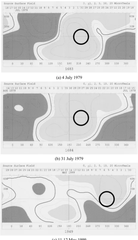
The low-density solar winds on 4 and 31 July 1979 were observed in the away IMF sector while the 11–12 May 1999 event preceded a sector boundary. The event on 4 July 1979, recurred on 31 July 1979, suggesting that it was a corotating rather than a transient structure. In the events on 31 July 1979, and 11–12 May 1999, the density decreased gradually, and its recovery time was shorter than the time it took to decrease while the density decrease of the 4 July 1979 event looks symmetrical.

(b) 31 July 1979

(c) 11-12 May 1999

Fig. 8. Synoptic maps of source surface field made by the Wilcox Observatory. Circles show the probable source regions of three long-duration low-density solar wind events shown in Fig. 7.

the 11–12 May 1999 is suggested to be in the large positive polarity region.

4 Summary

We found that the duration of the low-density solar wind event of 11–12 May 1999 was 22 hours, making it the longest event in our database when we selected solar winds with density 0.5 cm−3 or less. Several low-density solar wind events have been observed since 1963. For those low-density events, plasma beta, Alfven Mach number, and dynamic

pres-solar wind data measured by the ACE spacecraft, Dr. D. J. Mc-Comas (Los Alamos National Laboratory) for the ACE/SWEPAM data, and Drs. N. F. Ness, L’Heureux, and C. W. Smith (Bartol Re-search Institute) and Drs. L. Burlaga and M. Acuna (NASA/GSFC) for the ACE/MAG data, the Wilcox Observatory for the synoptic maps of the solar source surfaces.

Topical Editor E. Antonucci thanks E. Cliver and another Ref-eree for their help in evaluating this paper.

References

Cairns, I. H., Fairfield, D. H., Anderson, R. R., Carlton, V. E. H., Paularena, K. I., and Lazarus, A. J., Unusual location of Earth’s bow shock on September 24-25, 1987: Mach number effects, J. Geophys. Res., 100, 47–62, 1995.

Fairfield, D. H., Average and unusual locations of the Earth’s mag-netopause and bow shock, Ann. Geophysicae, 76, 6700–6716, 1971.

Hundhausen, A. J., The solar wind, in Introduction to space physics, Eds. M. G. Kivelson and C. T. Russell, Cambridge Univ. Press, pp. 91–128, 1995.

Kawano, H., Russell, C. T., and Newbury, J. A., Correlation be-tween the solar wind dynamic and static pressures, J. Geophys. Res., 105, 7583–7589, 2000.

Lopez, R., Solar cycle invariance in solar wind proton temperature relationships, J. Geophys. Res., 92, 11189–11194, 1987. Newbury, J. A., Russell, C. T., Phillips, J. L., and Gary, S. P.,

Elec-tron temperature in the ambient solar wind: Typical properties and a lower bound at 1 AU, J. Geophys. Res., 103, 9553–9566, 1998.

Richardson, I. G. and Cane, H. V., Regions of abnormally low pro-ton temperature in the solar wind (1965–1991) and their associ-ation with ejecta., J. Geophys. Res., 100, 23397–23412, 1995. Sibeck, D. G., Lopez, R. E., and Roelof, E. C., Solar wind control of

the magnetopause shape, location, and motion, J. Geopys. Res., 96, 5489–5495, 1991.