Uncertain Interest Rate Modelling

(1)

Uncertain Interest Rate Modelling

David Epstein

St Catherine’s College

University of Oxford

A thesis submitted for the degree of

Doctor of Philosophy

(2)

Abstract

(3)

Acknowledgements

I would like to thank Paul Wilmott for his encouragement and guidance as my supervisor. In addition, many other members of the mathemati-cal finance group at Oxford have taken an interest in my work and I am grateful to them for numerous comments, discussions and advice. In par-ticular, Hyungsok Ahn, Mauricio Bouabci, Rich Haber, Amanda Hosken and Philipp Sch¨onbucher. I would also like to thank OCIAM, the EPSRC and the Smith Institute for their financial support over various periods of the last four years.

I have received a tremendous amount of support and encouragement from my family and friends during this time. In particular, the DH9 crew -Chris, Mark, Keith, (and more recently) Jim and John - and all of the coaches, athletes and parents from K.E.E.N., especially Angie, Ching, Fiona, Helen, Jacks, Rach and Steve.

(4)

Statement of originality

(5)

List of Figures

1.1 Diagramatic representation of a coupon and zero-coupon bond . . . . 3

1.2 Diagramatic representation of a swap . . . 4

1.3 Decomposition of a single floating rate payment . . . 4

1.4 Decomposition of the floating rate side of a swap . . . 5

1.5 Decomposition of a swap into zero-coupon bonds . . . 5

1.6 An interpolated yield curve . . . 9

1.7 The yield to maturity and forward rate . . . 11

2.1 The interest rate paths for a zero-coupon bond under our simple model 20 2.2 The interest rate path for a coupon bond under our simple model. . . 22

2.3 The interest rate paths for a zero-coupon bond under our non-probabilistic model . . . 24

2.4 Possible interest rate paths for a coupon bond under our non-probabilistic model . . . 26

2.5 The worst-case increase and risk-free increase for a contract . . . 27

2.6 Characteristics for the linear problem . . . 30

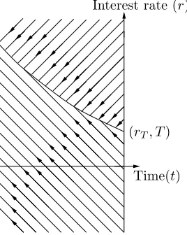
2.7 Multiple characteristics when there is a maximum at (rT, T) . . . 32

2.8 Evolution of a maximum without discounting . . . 33

2.9 Characteristics when there is a maximum at (rT, T) and we introduce a shock . . . 33

2.10 The local problem with a maximum at (rT, T) . . . 34

2.11 The incomplete set of characteristics originating from a minimum . . 38

2.12 Evolution of a minimum without discounting . . . 38

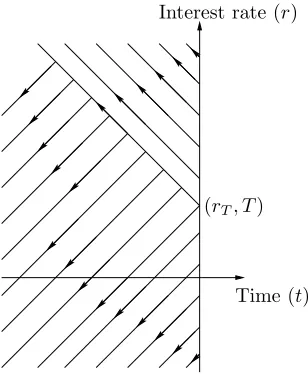
2.13 The complete set of characteristics with a minimum at (rT, T) . . . . 40

2.14 The local problem with a minimum at (rT, T) . . . 41

2.15 Evolution of a pair of a maximum and a minimum . . . 44

2.16 Characteristics for the pair of a maximum and a minimum . . . 45

2.17 Characteristics with an inflection point at (rT, T) . . . 46

(10)

2.19 Characteristics with various inflection points . . . 48

2.20 Characteristics with boundaries . . . 49

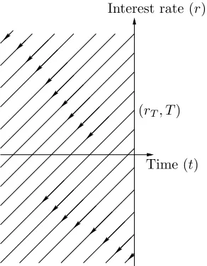
3.1 Characteristics when Vr(r, T)<0 . . . 52

3.2 Contract value with 0, 1, 2, 3, 4, 5 years to maturity . . . 53

3.3 Possible characteristics when Vr(r, T)>0: Case I . . . 54

3.4 Contract value in Case I . . . 55

3.5 Possible characteristics when Vr(r, T)>0: Case II . . . 56

3.6 Contract value in Case II . . . 57

3.7 Possible characteristics when there is an interior maximum: Case I . . 59

3.8 Contract value in Case I for a ‘linear’ maximum . . . 61

3.9 Contract value in Case I for a ‘quadratic’ maximum . . . 61

3.10 Possible characteristics when there is an interior maximum: Case I . . 62

3.11 Possible characteristics when there is an interior maximum: Case II . 62 3.12 Contract value in Case II for a ‘linear’ maximum . . . 64

3.13 Contract value in Case II for a ‘quadratic’ maximum . . . 64

3.14 Possible characteristics when there is an interior minimum: Case I . . 65

3.15 Contract value in Case I for a ‘linear’ minimum . . . 67

3.16 Contract value in Case I for a ‘quadratic’ minimum . . . 68

3.17 Possible characteristics when there is an interior minimum: Case II . 68 3.18 Contract value in Case II for a ‘linear’ minimum . . . 70

3.19 Contract value in Case II for a ‘quadratic’ minimum . . . 70

4.1 Zero-coupon bond value in a worst-case scenario . . . 75

4.2 Zero-coupon bond value in a best-case scenario . . . 75

4.3 Yield in a worst-case scenario for the zero-coupon bond . . . 76

4.4 Yield in a best-case scenario for the zero-coupon bond . . . 76

4.5 Spread in zero-coupon bond yields . . . 77

4.6 Hedging a contract with a zero-coupon bond . . . 78

4.7 Value of a 5 year zero-coupon bond when we hedge with λ of a 1 year zero-coupon bond . . . 81

4.8 Hedging a contract with market-traded instruments . . . 82

4.9 Interest rate paths for the 4 yr bond optimally hedged in (a) a worst-case scenario and (b) a best-worst-case scenario . . . 84

4.10 Yield Envelope with hedging . . . 87

4.11 Yield in a worst-case scenario for the zero-coupon bond . . . 88

(11)

4.13 The yield curve for the bonds from Table 4.1 . . . 90

4.14 Cashflows of the leasing portfolio . . . 96

4.15 The current yield curve for the leasing portfolio . . . 97

4.16 The hedging cashflows for the leasing portfolio . . . 99

5.1 Worst- and best-case prices for the underlying zero-coupon bond . . . 101

5.2 Value of the call option . . . 102

5.3 Pricing a bond option in a worst-case scenario . . . 103

5.4 A more general approach to option pricing . . . 108

5.5 European put option value in a worst-case scenario . . . 110

5.6 Pricing American options . . . 112

5.7 American put option value in a worst-case scenario . . . 114

5.8 The amortising schedule . . . 121

5.9 The swap yield curve . . . 122

5.10 Convertible bond value with constant interest rate . . . 125

6.1 A possible evolution ofr and r0_{, the ‘real’ rate . . . 132}

6.2 Value of a 4 year zero-coupon bond with varying . . . 134

6.3 Examining data to choose a sensible value for . . . 136

6.4 (a) An inconsistent use of the uncertainty bars, (b) The consistent picture136 6.5 1 month US interest rate data . . . 137

6.6 Value of a 4 year zero-coupon bond with a crash allowed . . . 140

6.7 Illiquid Yield Envelope . . . 145

A.1 The discretised solution space . . . 155

A.2 The explicit finite difference scheme . . . 156

(12)

List of Tables

4.1 The zero-coupon bonds with which we hedge . . . 83

4.2 Value of a 4 year zero-coupon bond . . . 84

4.3 The optimal static hedges for a 4 year zero-coupon bond . . . 84

4.4 Hedging a zero-coupon bond with maturity T . . . 86

4.5 The hedging bonds for Figures 4.11 and 4.12 . . . 87

4.6 Value of the decomposed swap . . . 90

4.7 The optimal static hedges for the decomposed swap . . . 91

4.8 Value of the approximated swap . . . 91

4.9 The optimal static hedges for the approximated swap . . . 91

4.10 Value of a cap with varying strike . . . 93

4.11 Value of a floor with varying strike . . . 94

4.12 The benchmark bonds . . . 97

4.13 Present value of the portfolio with parallel shifts in the yield curve . . 98

4.14 The optimal hedge for the worst-case scenario portfolio valuation . . 98

5.1 Value of a European call option hedged with the underlying . . . 105

5.2 Value of a European put option hedged with the underlying . . . 105

5.3 Value of the optimally-hedged European call option . . . 109

5.4 The optimal static hedges for the European call option . . . 109

5.5 Value of the optimally-hedged European put option . . . 109

5.6 The optimal static hedges for the European put option . . . 109

5.7 Value of an American put option hedged with the underlying . . . 113

5.8 Value of the optimally-hedged American put option . . . 113

5.9 The optimal static hedges for the American put option . . . 114

5.10 The par-value hedging swaps . . . 118

5.11 Value of an eight-choice swap . . . 118

5.12 The optimal static hedges for the eight-choice swap . . . 118

(13)

5.15 Sensitivity of the index amortising rate swap value to parallel shifts in

the yield curve . . . 123

5.16 The yields for the zero-coupon bonds used to price/hedge the convert-ible bond . . . 126

5.17 Sensitivity of the convertible bond value to parallel shifts in the yield curve . . . 126

5.18 Sensitivity of the Vasicek model to shifts ina . . . 126

5.19 Sensitivity of the Vasicek model to shifts inb . . . 127

5.20 Sensitivity of the Vasicek model to shifts inν . . . 127

5.21 Sensitivity of the Vasicek model to shifts inb . . . 127

5.22 Sensitivity of the Vasicek model to shifts inν . . . 127

5.23 Optimal static hedge for the convertible bond . . . 129

5.24 Added value due to convertability . . . 129

6.1 Worst-case value of a 4 year zero-coupon bond with an uncertainty band134 6.2 The optimal static hedges for a 4 year zero-coupon bond with an un-certainty band . . . 134

6.3 Worst-case value of a 4 year zero-coupon bond with crashes allowed . 139 6.4 The optimal static hedges for a 4 year zero-coupon bond with crashes allowed (example 1) . . . 140

6.5 The optimal static hedges for a 4 year zero-coupon bond with crashes allowed (example 2) . . . 142

6.6 The largest changes in the 1 month daily interest rate data . . . 143

6.7 The hedging bonds with a bid-offer spread . . . 144

(14)

Chapter 1 Introduction

In contrast to the asset price world, there is no commonly accepted model for the movement of the underlying in the interest rate world. Consequently, there are a number of different approaches to the pricing of fixed-income products.

The simplest approach is to price a product off a yield curve. This method is effective for simple contracts, bonds for instance. However, for more complex prod-ucts, where optionality or convexity play a role, the precise nature of the interest rate movements is significant and so the method does not give accurate results.

The ‘traditional’ approach to pricing these more complicated products is to in-troduce stochastic variables to model a number of ‘unknown’ factors, on which we believe the interest rate movements depend. These models can be single- or multi-factor models for the movement of the short-term interest rate, or models for the movement of the whole yield curve (the Heath, Jarrow & Morton approach). All of these methods rely on the estimation of parameters. Not only are these parameters (for instance, volatility) difficult to estimate, but they can also be unstable [2].

The single- and multi-factor models have the additional disadvantages that they can require fitting to the current yield curve, again in an unstable fashion, and that they can assume an equally difficult to estimate and unstable correlation between yields of different maturities.

In the following work, we present an alternative approach to the pricing of fixed-income products. We introduce a non-stochastic non-probabilistic model for the short-term interest rate. This work has, in part, been inspired by the work on uncer-tain volatility in equity derivatives by Avellaneda, Levy and Paras [4] and Lyons [48]. However, the ideas cannot be directly translated into the interest rate world, because the underlying that we consider is not a traded quantity.

(15)

what is possible and what is not. Clearly, there are therefore going to be a number of possible paths that the short rate could take. For each path, when we use the short rate as a discount rate, the contract in question could have a different value (where we consider the position of the holder of the contract). We will consequently find a range of possible values for the price of a contract. We identify the lowest of these as the ‘worst-case scenario value’.

The analysis of this worst-case valuation problem leads to a nonlinear, first-order, hyperbolic partial differential equation. We can solve this equation either analytically or via numerical methods. The results motivate us to investigate whether there is any role for hedging. Rather than dynamic hedging, we find that there is an optimal static hedge for a product [15], [21], [26], [27]. This form of hedging mirrors the yield curve fitting that is often applied to stochastic interest rate models, but has none of the associated problems with inconsistency.

There are a number of practical applications for this model. Clearly, it can be used to find price ranges for instruments and spot potential arbitrage opportunities in the market [30], [32], [33]. If we have an over-the-counter (OTC) contract - one that is not listed in the market - then we can use the uncertain interest rate model to construct an optimal static hedge of market-traded products and reduce the inherent interest rate risk [34], [35]. Finally, we can use the model as a risk management tool. With a sensible choice of parameters, it is possible to show that the model is completely consistent with past interest rate history. In this case, the worst-case scenario value is a definitive lower bound for the value of a portfolio. The same consistency cannot easily be shown for any other model [31], [36].

In the next section, we present a review of the common fixed-income products available in the market and of the traditional approaches and techniques used to price them, some of which we will use for comparison later on. We then summarise the theory of uncertain volatility in the equity world, which is analogous to our uncertain interest rate theory. Finally we present an outline of the contents of the thesis.

1.1 Common fixed-income contracts

(16)

1.1.1 Bonds

A bond is a borrowing arrangement in which a borrower (the writer) issues an IOU to an investor (the holder). In its simplest form, it only requires the writer to pay a specified amount, the principal, to the holder, at a specified date in the future, the maturity. This contract is called a zero-coupon bond.

The more general contract, the coupon bond, also requires the writer to make interim payments, or coupons, of a specified proportion of the principal, the coupon rate, at specified dates, up to and including the maturity of the bond, as well as paying the principal at maturity.

Figure 1.1 shows a diagramatic representation of a zero-coupon bond and a coupon bond. Horizontal distance represents time, with maturity at the right hand end. Each arrow represents a cashflow. Arrows above the horizontal axis represent positive cashflow payments from the writer to the holder, and those below the axis represent negative payments. An arrow with a straight shaft is indicative of a payment of a known quantity at the origination of the contract, whereas an arrow with a wavy shaft (as we will see for the next contract) is indicative of a cashflow which is dependent on some quantity that is not known at the origination of the contract (for instance, an interest rate).

Zero-coupon bond

Coupon bond

Figure 1.1: Diagramatic representation of a coupon and zero-coupon bond

1.1.2 Swaps

(17)

payment date is called a swaplet. We can express these cashflows mathematically as

P(r−rf), (1.1)

where P is the principal, r is the reference rate andrf is the fixed rate.

The contract must specify which interest rate is to be used, and at what time it is to be measured, since this may be prior to the payment date [25]. The fixed rate is usually chosen so that there is no premium payable to either party at the origination of the contract (in this case, the contract is called a par swap). Figure 1.2 shows a diagramatic representation of a swap where the holder receives the floating payments and pays the fixed.

Swap

Figure 1.2: Diagramatic representation of a swap

In certain circumstances, it is possible to decompose a swap into a portfolio of zero-coupon bonds. Consider a single floating rate payment, as shown in Figure 1.3.

=

Tc Tc Tc−τ Tc

1 r

τ

1 +

r

τ

1

Figure 1.3: Decomposition of a single floating rate payment

If the floating rate is the interest rate for a period ofτ and is measured at a time

τ before the payment date, Tc, then a cashflow of 1 at the date Tc −τ is equivalent

to a cashflow of 1 +rτ at the date Tc, since rτ is the τ period interest rate. We can

(18)

=

Floating rate side of swap

Figure 1.4: Decomposition of the floating rate side of a swap

=

Swap

Figure 1.5: Decomposition of a swap into zero-coupon bonds

The swap, as a whole, can therefore be expressed as a sum of zero-coupon bonds, as shown in Figure 1.5. If this swap has N payment dates, at times T1(=τ), T2, . . . , TN,

then we can write the value of the swap in terms of the fixed interest rate, rf, and

zero-coupon bonds, as

P 1−Z(t;TN)−rf N

X

i=1

Z(t;Ti)

!

,

where Z(t;T) is the value at time t of a zero-coupon bond with principal 1 and maturity at timeT. For a par swap, we must choose rf so that the swap initially has

no value, i.e.

rf =

1−Z(t;TN)

PN

i=1Z(t;Ti)

.

(19)

is a τ-period rate. To annualise the rate, we must divide by τ (assuming that τ is measured in years).

1.1.3 Caps and floors

Caps and floors are interest rate agreements whereby one party (the writer), for an upfront premium, agrees to compensate the other (the holder) at specific dates if a designated interest rate, the reference rate, differs from a predetermined level [19]. The agreement is called a cap if payment occurs when the reference rate exceeds a predetermined level. The agreement is called a floor if payment occurs when the reference rate falls below a predetermined level. The predetermined level is called the strike rate.

The individual set of cashflows for a particular cap payment date is called a caplet. We can express these cashflows mathematically as

P max(r₋rs,0), (1.2)

where P is the principal, r is the reference rate andrs is the strike rate.

The individual set of cashflows for a particular floor payment date is called a floorlet. We can express these cashflows mathematically as

P max(rs−r,0). (1.3)

As with the swap contract, a cap or floor contract must specify which interest rate is to be used, and at what time it is to be measured. It is again possible to decompose the contract. In this case, into a portfolio of bond options. First of all, we define a bond option.

1.1.4 Bond options

A vanilla bond option is a contract that gives the holder the right, but not the obligation, to buy or sell a bond to the writer at, or between prescribed times, for a specified price. A European option gives the holder this right at a specified date in the future (the expiry). An American option gives the holder the right at all times until expiry.

A call option gives the holder the right to buy the prescribed bond (the under-lying) for a prescribed amount (the exercise price). This payoff can be expressed mathematically as

(20)

where B is the value of the bond at expiry of the option and E is the exercise price (since we only exercise the option if B > E at expiry).

A put option gives the holder the right to sell the prescribed bond for a prescribed amount. This payoff can be expressed mathematically as

max(E−B,0). (1.5)

1.1.5 Decomposition of caps/floors into bond options

We consider a single caplet, with a floating rate that is the interest rate for a period of τ and is measured at a timeτ before the payment date,Tc. In this case, a cashflow

of 1 at the date Tc−τ is equivalent to a cashflow of 1 +rτ at the dateTc, sincerτ is

the τ period interest rate. (We assume, without loss of generality, that the principal is 1).

The caplet has cashflow

max(rτ −rs,0),

received at time Tc. This is equivalent to a cashflow of

1 1 +rτ

max(rτ −rs,0),

received at time Tc−τ. We can rewrite this as

max

1₋ 1 +rs 1 +rτ

,0

,

where we can think of

1 +rs

1 +rτ

,

as being the price at time Tc −τ of a bond that pays out 1 +rs at time Tc. We can

therefore consider the caplet to be equivalent to a put option, with this bond as the underlying, with exercise price 1 and expiry at timeTc−τ. Hence, we can decompose

a cap into a portfolio of put options.

Similarly, we can decompose a floor into a portfolio of the corresponding call options.

1.2 Traditional approaches to interest rate

modelling

(21)

definitions and methods and, in detail, only those which we will refer to during this thesis. Further details of all these approaches can be found in a number of sources, for instance, Hull [44] or Wilmott [63].

1.2.1 Arbitrage

An arbitrage opportunity is the opportunity to make a risk-free profit. We shall assume that there is an absence of such arbitrage opportunities throughout this work.

1.2.2 Present value

The present value (at time t) of an amount of cash E to be received at time T is the amount we would pay now for this future cash flow. To find the present value of the cash flow, we must discount it using a specified interest rate. If we have a continuously-compounded short-term interest rate, r, then money invested in the bank, M(t), grows exponentially according to

dM =rM dt.

When this short interest rate is a known function of time, r(t), and M(T) =E then we can solve the resulting ordinary differential equation to find

M(t) = Ee−RtTr(τ)dτ. (1.6)

(Note that throughout this work, we shall assume that the short-term interest rate is continuously-compounded).

1.2.3 Yield to maturity

The yield to maturity is a measure of the rate of return of a bond held until maturity. It is the constant interest rate that we would have to use to discount all of the bond’s cashflows to value the bond at its current market price.

For a zero-coupon bond, with principalP, expiry at timeT and market priceZM,

the yield to maturity at time t is

Y =−log (ZM/P)

T −t . (1.7)

(22)

Figure 1.6 gives an example of a yield curve constructed with linear interpolation and one constructed with spline interpolation [1] between the points where the yields have been calculated (the x’s).

x x

x

Maturity

x x

x

Maturity

Linear interpolation Spline Interpolation

Yield Yield

Figure 1.6: An interpolated yield curve

1.2.4 Pricing off the yield curve

We can price a product off the yield curve as long as all of its cashflows are known quantities at the origination of the contract. To do this, we just add up the present values of all the cashflows. To find the present value of a cashflow, we read off the rate of return for the payment date of the cashflow from the yield curve and discount the cashflow at that rate.

However, it is possible to find two instruments with the same maturity but different yields, for example, two coupon bonds with the same maturity but different coupon structures. It is not possible to construct a yield curve consistent with both of these instruments.

In addition, we assume that a yield is constant from now until maturity, so we cannot use this rate to evaluate any cashflow that depends on an interest rate of shorter term, for instance, a swap.

(23)

1.2.5 Forward rates

Forward rates are interest rates that apply over given periods of time and are consis-tent with all our yield data. If we have a continuous set of zero-coupon bond prices, for all maturities, Z(t;T), then the implied forward rate is the short rate curve that is consistent with all of these prices, F(t;T), and satisfies

Z(t;T) =e−RtTF(t;τ)dτ. (1.8)

We can differentiate this equation to find

F(t;T) =₋ ∂

∂T(logZ(t;T)). (1.9)

If we have a finite set of zero-coupon bonds from which we want to generate our forward rate curve, then we use the following methodology:

• Rank the bonds in order of increasing maturity, T1, T2, . . . , TN.

• Find the constant interest rate that must apply between now andT1, implied by

the market value of the first bond. This is the forward rate that holds between now and T1.

• Find the constant interest rate that must apply between T1 and T2, implied

by the market value of the second bond, when we apply the first forward rate between now and T1. This is the forward rate that holds between T1 and T2.

• For theith forward rate, find the constant interest rate that must apply between

Ti−1 and Ti, implied by the market value of the ith bond, when we apply the

previous forward rates between the appropriate times. This is the forward rate that holds between Ti−1 and Ti.

• Repeat the previous step as necessary.

This method is called bootstrapping. Figure 1.7 shows the forward rate curve generated from the yield data used to construct the yield curves of Figure 1.6. We include the yields of all the instruments for comparison.

(24)

x x

x

Yield

Maturity

Forward rate

Maturity

Figure 1.7: The yield to maturity and forward rate

we must make some additional assumptions, grouping some of the cashflow dates, for instance.

We also note that rather than a piecewise constant forward rate curve, we could instead construct a continuous curve, using some form of interpolation.

1.2.6 Pricing off the forward rate curve

We can use the forward rate curve to price any simple fixed-income contract. As with yield curve pricing, we again just add up the present values of the cashflows. If we have a forward rate curve, F(t;T), and a cashflow C(r) at time Tc, then the present

value, at time t, of the cashflow is

C(F(t;Tc))e−

RTc

t F(t;τ)dτ. (1.10)

However, this method is still inappropriate for more complex products, such as caps, floors or bond options, whose values depend more strongly on the exact nature of the underlying interest rate movements. To price these contracts, we must first construct a model for the interest rate.

1.2.7 Stochastic models

A popular approach to interest rate modelling is to construct a stochastic model for the movement of the short-term interest rate. We can then price a contract as the expected value of its cashflows, where we discount at this short rate, and also use the rate to value any rate-dependent cash flows, i.e.

V =XE∗hC(r)e−RtTirτdτ

i

(25)

where the contract has cashflows Ci(r) at times Ti and we take the risk-neutral

ex-pectation, E∗_t [53], [56].

1.2.8 One-factor models

The simplest of these stochastic models are one-factor models. Many such models have been proposed [11], [23], [28], [39], [58]. They assume that interest rate movements are driven by a single random factor. They have the general form

dr=u(r, t)dt+v(r, t)dX, (1.12)

whereuandvare some specified functions ofrandtanddX is a Wiener process (that is, a random variable drawn from a Normal distribution with mean 0 and variance

dt).

We can derive a pricing equation for the value of a fixed income product under this model. We find that the price of a contract, V(r, t), satisfies

Vt+ 1₂v2Vrr+ (u−λv)Vr−rV = 0, (1.13)

where λ is the market price of risk [65].

This is a second-order, parabolic, partial differential equation. It has final condi-tion V(r, T) given by the value of the contract at maturity and boundary conditions which depend on the specification of the contract. We include a cashflow at time Tc

as a jump condition (due to an absence of arbitrage opportunities) of the form

V(r, T_c−) =V(r, T_c+) + Λ(r), (1.14)

when there is a cashflow Λ(r) at time Tc and where the superscript ‘−’ denotes just

before the cashflow date and ‘+’ just after.

The market price of risk is the ratio of the excess return above the risk-free rate to the level of risk inherent in a portfolio. The increase in the value of the portfolio over a time step dtis an extraλdtfor each unit of risk,dX. It is necessary to introduce such a measure because the underlying process, the short rate, is not a traded quantity.

(26)

1.2.8.1 Vasicek

In the Vasicek model, we set

u(r, t) =a₋br and v(r, t) =ν,

(where a,b and ν are constants), so that the short rate is mean-reverting to the level

a/b at a rate b [61]. In this case, the short rate process satisfies

dr= (a−br)dt+νdX.

We can generalise this model by allowing a and b to be functions of r and t. In the extended Vasicek model of Hull & White, a is time-dependent, so that

dr= (a(t)₋br)dt+νdX. (1.15)

If we estimate b and ν, then we can choose a(t) to fit the current yield curve (i.e. so that the theoretical and actual market bond prices coincide). To fit the yield curve at time t∗, we find that a(t) must satisfy

a(t) =₋∂

2

∂t2 log(ZM(t

∗_;_t₎₎₋_b∂

∂tlog(ZM(t

∗_;_t_{)) +} c2

2b 1−e

−2b(t−t∗₎

, (1.16)

where ZM(t∗, T) is the market price of the T-maturity zero-coupon bond at time t∗

[42], [43].

1.2.8.2 ACKW

The ACKW model is an empirical model of the short rate, proposed by Apabhai, Choe, Khennach and Wilmott [2]. Rather than choosing a model that has tractable solutions, they consider a general form for the short rate model and perform an empirical analysis of short rate data to choose the precise parameters. They assume that

u(r, t) = ν2_r2β−1

β₋ 1

2 −

1

2a2 log(r/r¯)

and

v(r, t) =νrβ,

so that the short rate process is

dr =ν2r2β−1

β−1

2 −

1

2a2 log(r/r¯)

(27)

They then perform a statistical analysis of US short rate data to choose the model parameters, and find that

β= 1.13 andν = 0.126, (1.18)

from an examination of the expected average value of (δr)2_{, and that}

a= 0.4 and ¯r= 0.08, (1.19)

by considering the steady-state probability density function for the short rate. The model is therefore approximately lognormal and mean-reverts to 8%.

1.2.9 Multi-factor models

The simplest generalisation of the one-factor stochastic model is the multi-factor model. This assumes that movements in the yield curve depend on more than one random factor. If an instrument depends on the difference between different sections of the yield curve, rather than just its level, then we need at least a second source of randomness to model this movement effectively [18], [46], [47].

Generally, we model the short-term interest rate, r, along with another indepen-dent variable, l, where

dr=udt+vdX1, (1.20)

and

dl =pdt+qdX2. (1.21)

u, v, p and q are some specified functions of r, l and t and dX1 and dX2 are

ran-dom variables drawn from Normal distributions with mean 0 and variance dt, with correlation ρ.

We can derive a pricing equation for the value of a fixed income product under this model. We find that the price of a contract, V(r, l, t), satisfies

Vt+1₂v2Vrr+ρvqVrl+1₂q2Vll+ (u−λrv)Vr+ (p−λlq)Vl−rV = 0, (1.22)

(28)

1.2.10 Heath, Jarrow & Morton

All of the previous stochastic models have been models of the movement of one or more interest rate factors. However, Heath, Jarrow & Morton suggest a more general approach, by modelling the movement of the whole forward rate curve [38]. The method consistently reproduces the current yield curve, since this information is contained in the initial forward rate curve.

We assume that zero-coupon bonds evolve, in a risk-neutral world, according to

dZ(t;T) =r(t)Z(t;T)dt+σ(t, T)Z(t;T)dX. (1.23)

We can then determine the stochastic differential equation for the evolution of the risk-neutral forward rate curve

dF(t;T) =

ν(t, T)

Z T t

ν(t, s)ds

dt+ν(t, T)dX, (1.24)

where

ν(t, T) =₋ ∂

∂Tσ(t, T). (1.25)

Since

r(t) =F(t;t) =F(t∗;t) +

Z t t∗

dF(τ;t), (1.26)

we can also find the short rate for any time t in the future of today, t∗_.

Using this information, we can price a contract by calculating the present value of all of its cashflows. To do this, we must first choose a specific form for σ and then either proceed analytically, or implement a Monte Carlo method to simulate the various forward and short rate paths [22].

We remark that more recently, Brace, Gatarek and Musiela have proposed a sim-ilar model for a non-infinitessimal short rate, BGM, which can be used to model discrete (and observable) forward rates directly [16].

1.3 The uncertain volatility model

In the final section of this review, we present the uncertain volatility model for equity derivatives. Our motivation for including this model is that it was one of the original inspirations for the form of our uncertain interest rate model.

(29)

where µand σ are known parameters, and dX is drawn from a Normal distribution with mean 0 and variance dt.

It is then possible to derive a pricing equation for the value of an equity derivative,

V(S, t), of the form

Vt+1₂σ2S2VSS +rSVS−rV = 0, (1.28)

with appropriate final and boundary conditions for the specific contract.

In the uncertain volatility model, we generalise the assumption that σ is known, to allow σ to lie anywhere within a given range,

σ− ≤σ≤σ+, (1.29)

Since there is a range of possible values forσ, we find that there is a range of possible values for the equity derivative. We identify the lowest of these as the worst-case scenario value and find that it is possible to derive the following nonlinear, second-order, parabolic differential equation for this value,

Vt+ 1₂σ2(VSS)S2VSS +rSVS−rV = 0, (1.30)

where

σ(X) =

σ+ _if _{X <}₀

σ− _if _{X >}₀_. (1.31)

Since this is a nonlinear problem, the value of a portfolio of contracts is not necessarily the same as the sum of their individual values. The price of a product therefore depends on what it is hedged with. Consequently, we can statically-hedge an OTC contract with market-traded contracts and find that there is an optimal static hedge which gives the OTC contract the highest possible worst-case scenario value [3], [6].

We remark that Avellaneda and Lewicki have also applied this approach to in-terest rate modelling, where they propose a Heath, Jarrow & Morton model with an uncertain volatility [5]. In the following work, we will eliminate the consideration of volatility altogether and propose a more general form of uncertain model for the interest rate.

1.4 Overview

(30)

model, we prescribe bounds on both the short-term interest rate and its growth rate. We derive the partial differential equation for the worst-case scenario value of a contract under this model and find that it is first-order, nonlinear and hyperbolic. We then examine the solution of this equation via the method of characteristics.

We illustrate the solution by the method of characteristics in Chapter 3. We first discuss the general methodology and then considered various examples of final data. In each case, we consider all of the possible characteristic pictures that could occur and find the solution of the equation for each of these situations.

We begin Chapter 4 with a discussion of the consequences of the nonlinearity of our pricing equation and consider the problem of the contract value in a best-case scenario. Using the zero-coupon bond to illustrate the procedure, we then consider in detail the pricing and hedging of a contract. We show that there is an optimal static hedge for which the worst-case scenario value of the contract reaches a maximum level. Similarly, there is another optimal static hedge for which the best-case scenario value of the contract reaches a minimum level. Associated with these results is the Yield Envelope. This is similar in form to the yield curve, however, at a maturity where no traded contract exists, there is a yield spread. We then apply the model to the pricing and hedging of swaps, caps and floors, describing the appropriate jump and final conditions for the pricing equation in each case. Finally, in the light of these results, we discuss possible applications for the model and price and hedge a real-world leasing portfolio.

In Chapter 5, we apply our model to the pricing and hedging of more exotic fixed-income contracts. We begin with the European bond option and derive two different methodologies for the pricing of the option, dependent on the type of the option and the hedging strategy to be followed. Second, we price the multi-choice swap, a contract with embedded decisions. This swap allows the holder to choose on which

m of theM possible cashflow dates to exchange interest rate payments. To price this contract, we introduce a set of functions for the contract value, dependent on how many cashflows there are left to take.

(31)

We describe the partial differential equation for the worst-case value of the bond and compare the results of the pricing process to a number of more traditional approaches to interest rate modelling.

In Chapter 6, we present extensions to our uncertain model. These allow for interest rate paths that are indistinguishable from those seen in practice. We consider the concept of the uncertainty band, in which our model for the short-term interest rate becomes an estimate of the real short-term rate. We derive the new partial differential equation for the worst-case value of a contract under this assumption and describe how to relate the short-term interest rate to rates of a longer period. Using this concept, we can examine past interest rate data to choose a sensible width for the band. As a further extension, we include the possibility for crashes in the short-term interest rate. These crashes can take one of two forms. There can either be a maximum possible total number or a maximum possible frequency for the crashes. We describe the pricing equation framework for each case and then re-examine the data to find an adjusted uncertainty bandwidth, along with sensible parameters for these events. To close the chapter, we study the effect of illiquidity of the hedging instruments on the worst-case scenario valuation of a contract and present an illiquid version of the Yield Envelope.

(32)

Chapter 2 An uncertain interest rate model

In this chapter, we present a non-probabilistic model for the short-term interest rate. We use this as a discount rate to price fixed-income products. If a contract has cashflows Ci(r) at timesTi then the present value of the contract under this model is

X

i

Ci(r(Ti))e−

R_Ti

t r(τ)dτ, (2.1)

where r(t) is the evolution of the short-term interest rate over the maturity of the contract.

We will place bounds on the possible movements of the short rate. Consequently, there will be a range of possible prices for a fixed-income contract, since there will be a number of possible paths for the short rate and each of these could give the contract a different present value. We identify the lowest of these prices as the worst-case scenario value (for the holder of the contract). Under our short rate model, the contract must be worth at least this much, regardless of which path the short rate actually takes. We remark that the worst-case scenario for the holder of the contract will be the best-case scenario for the writer of the contract (the best-case scenario is discussed in Section 4.2). In this thesis, we will always consider the case of the holder of the contract. In the next section, we motivate this concept using the simplest possible model.

2.1 A simple example of worst-case scenario

valuation

(33)

where r+ _and _r− _{are constants. This means that it is possible for} _r _{to jump}

instan-taneously from any value to any other value within the range [r−, r+_]_.

2.1.1 Pricing a single cashflow

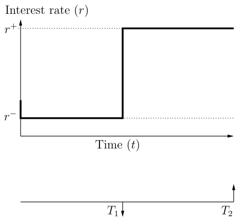
Consider a zero-coupon bond with principal P that matures at time T. We want to find the value of this bond in a worst-case scenario, at time t. This value will depend on the evolution of the short rate, r, in the intervening period.

Since there is only a single cashflow to consider, it is simple to identify the worst-case path for the interest rate. If the cashflow is positive, then the worst-worst-case scenario will occur when the interest rate is always as high as possible, so that the present value of the cashflow is as low as possible. However, if the cashflow is negative, then the worst-case scenario will occur when the interest rate is always as low as possible. Therefore, ifP >0 then the worst-case scenario occurs whenrimmediately jumps from its initial value to r+ _{and remains at this rate until maturity. In this case, the}

value of the bond is then

P e−r+(T−t).

If P < 0 then the worst-case scenario occurs when r instantaneously falls to r− and stays there until maturity. The value of the bond is then

P e−r−(T−t).

Figure 2.1 shows the evolution of the interest rate in a worst-case scenario for these two cases of zero-coupon bond valuation.

Time (t)

r+

r−

r+

r−

Time (t)

Interest rate (r) Interest rate (r)

T T

(34)

2.1.2 Pricing two cashflows

Now, let us make the problem slightly harder. We consider a coupon bond that has a cashflow of C at timeT1 andP at maturity,T2 (T1 < T2). This is equivalent to two

zero-coupon bonds, one with a principal of C and maturity at time T1 and the other

with a principal of P and maturity at timeT2.

If both cashflows are of the same sign, then the problem reduces to that of the previous section for a single cashflow. If the cashflows are positive, then the worst-case scenario will occur when the interest rate is always as high as possible, and if the cashflows are negative, then the worst-case scenario will occur when the interest rate is always as low as possible.

Consequently, If C > 0 and P > 0 then the worst-case scenario occurs when r

immediately jumps to r+ _{and stays there until maturity. The value of the bond at}

time t is then

Ce−r+(T1−t)₊_{P e}−r+(T2−t)_.

If C < 0 and P < 0 then the worst-case scenario occurs when r instantaneously falls to r− _{and stays there until maturity. The value of the bond in a worst-case}

scenario is then

Ce−r−(T1−t)₊_{P e}−r−(T2−t)_.

But what if the cashflows are of opposite sign? By way of illustration, we consider the case where C < 0 andP > 0. Since the latter cashflow is positive, the worst-case scenario will occur when the interest rate is always as high as possible between the two cashflow dates, T1 and T2. We must then examine the present value of the sum

of the two cashflows at the first cashflow date. If this value is still positive, then the worst-case scenario will occur when the interest rate is always as high as possible from now until the first cashflow date. However, if this value is negative, then the worst-case scenario will occur when the interest rate is always as low as possible from now until the first cashflow date.

Under our simple model, r can instantaneously jump from one value to another. Therefore, in the worst-case scenario, the interest rate will be r+ _between_T

1 and T2.

This is because it will be possible for the interest rate to jump to r+ _{at time} _T

1,

regardless of what value it takes between t and T1. The present value of the second

cashflow at time T1 is then

P e−r+_(T₂₋_T₁₎

(35)

The present value of the two cashflows at time T1 is therefore

C+P e−r+(T2−T1)_.

If C+P e−r+_(T

2−T1) _> _{0, then the worst case-scenario occurs when the interest rate}

immediately jumps to r+ _{(at time} _t_{) and stays there until}_T

2. The value of the bond

at time t is therefore

Ce−r+(T1−t)₊_{P e}−r+(T2−t)_.

However, if C + P e−r+_(T

2−T1) _< _{0, then the worst case-scenario occurs when the}

interest rate immediately jumps to r− (at time t) and stays there until T1 when it

jumps to r+ _{and remains there until} _T

2. The value of the bond at time t is then

Ce−r−(T1−t)₊_{P e}−r−(T1−t)−r+(T2−T1)_.

This interest rate evolution is shown in Figure 2.2.

Time (t)

r+

r−

Interest rate (r)

T2

[image:35.595.192.422.365.581.2]

T1

Figure 2.2: The interest rate path for a coupon bond under our simple model.

(We note that if C+P e−r+_(T

2−T1) _{= 0, then the value of the bond today will be}

zero regardless of which path the interest rate takes betweentandT1. This is because

it is the present value of zero at time T1).

(36)

2.2 A model for the evolution of the interest rate

We now propose our non-probabilistic model for the evolution of the short-term in-terest rate. We assume thatr is continuous and has a given initial value,r(t). We do not describe a model for the actual behaviour of the short rate. Instead, we bound the possibilities by placing the following constraints on its movement:

r− ≤r≤r+, (2.3)

and

c− ≤ dr

dt ≤c

+_. _(2.4)

Equation (2.3) states that the short rate is bounded above and below. For instance, we could say that the short rate must be at least 3% and no more than 20%. However, the two bounds, r+ _and _r−_{, can be time dependent.}

Equation (2.4) places similar constraints on the change in the short rate. For instance, we could say that the short rate cannot increase or fall by more than 4% per annum. These two bounds, c+ _and _c−_{, can be dependent on both} _r _and _t_.

However, we assume that c+ _>_{0 and} _c−_<_0.

We remark that this model does not appear to replicate the locally unbounded growth seen in the traditional stochastic models for the short rate and, to some extent, observed in practice. Since we are trying to model a long-term behaviour, we are not so concerned with these short-term movements as they will not significantly affect the worst-case price. However, in Section 6.1, we address the problem by considering cer-tain modifications to our model. When we perform a statistical analysis of short-term interest rate data, we find that we can make this extended model indistinguishable from the actual underlying process.

2.2.1 Pricing a single cashflow

For the zero-coupon bond, with principal P at maturity T, there is still an obvious solution to the worst-case scenario valuation problem.

(37)

Therefore, ifP >0 then the worst-case scenario occurs when r increases from its initial value as quickly as possible (i.e. dr_dt =c+_{) until it reaches}_r+_{. It then remains}

at this rate until maturity.

Similarly, if P <0 then the worst-case scenario occurs when r decreases from its initial value as quickly as possible (i.e. dr

dt = c−) until it reaches r− and then stays

there until maturity.

The zero-coupon bond value is then given by

P e−RtTr(τ)dτ,

where r(t) is the realised short rate path for the particular case under consideration. Figure 2.3 shows the evolution of the interest rate in a worst-case scenario for these two cases of zero-coupon bond valuation. In this and the following figure, we assume that r−_, _r+_, _c− _and _c+ _{are constants.}

Time (t)

r+

r−

r+

r−

Time (t)

Interest rate (r) Interest rate (r)

T T

Figure 2.3: The interest rate paths for a zero-coupon bond under our non-probabilistic model

2.2.2 Pricing two cashflows

Now we consider the coupon bond, with a cashflow ofCat timeT1andP at maturity,

T2.

(38)

Therefore, ifC >0 andP >0 then the worst-case scenario occurs whenrincreases from its initial value as quickly as possible (i.e. dr_dt =c+_{) until it reaches}_r+ _{and then}

remains at this rate until maturity.

Similarly, ifC < 0 andP < 0 then the worst-case scenario occurs whenrdecreases from its initial value as quickly as possible (i.e. dr

dt =c−) until it reachesr− and then

stays there until maturity.

The coupon bond value is then given by

Ce−RtT1r(τ)dτ +P e−

RT₂

t r(τ)dτ,

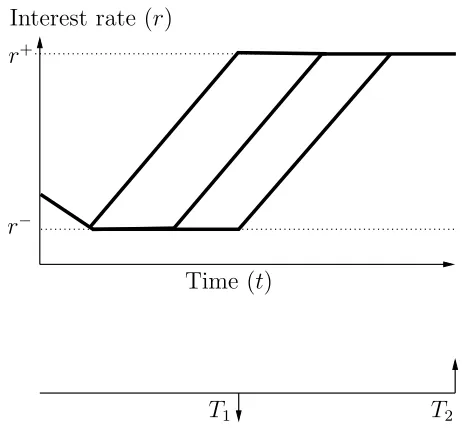
where r(t) is the realised short rate path for the particular case under consideration. But if the cashflows are of different sign, then the solution to the problem is far less obvious. By way of illustration, we again consider the case where C < 0 and

P > 0. Since the latter cashflow is positive, it will have least value when the interest rate is always as high as possible (between t and T2). On the other hand, the former

cashflow is negative and will have least value when the interest rate is as low as possible between t and T1.

If the interest rate were to remain at r+ _{for the entire period} _T

1 to T2 then the

present value of the second cashflow at time T1 would be

P e−r+(T2−T1)_.

If we include the first cashflow, then we find that the present value of the bond at time T1 would be

C+P e−r+(T2−T1)_.

If this value is positive, then the worst-case scenario occurs when r is always as high as possible over the entire period until maturity. The evolution of r will consequently be the same as for the case with solely positive cashflows. (Note that we have assumed a growth rate such that r can grow from its original value tor+ _before_T

1). However,

if the value is negative, then in the worst-case scenario, we need r to be as low as possible for all times preceding T1 and as high as possible for all times after T1.

Unfortunately,rcannot instantly jump from one value to another under this model and it is not clear at what time rshould start increasing fromr− _{to reach}_r+_{. Figure}

2.4 shows three plausible short rate evolutions. The outer paths are in some sense ‘bounding paths’. These paths either begin or end the change from r− _to_r+ _{at time}

T1. Since we want the interest rate to be as low as possible before T1 and as high as

(39)

Time (t)

r+

r−

Interest rate (r)

[image:39.595.192.423.104.319.2]

T1 T2

Figure 2.4: Possible interest rate paths for a coupon bond under our non-probabilistic model

However, there are still infinitely many possible paths, and only one may give the correct worst-case scenario value.

We must develop a method for establishing the realised interest rate over the period for which we want to perform a worst-case scenario valuation, or for directly calculating the value of a contract in this scenario. In the next section, we approach the problem from the perspective of the change in the contract’s value over a small time step dt and obtain a differential equation for the worst-case price.

2.3 The differential equation for

V

(

r, t

)

2.3.1 The formulation of the differential equation

LetV(r, t) be the value of our contract, when the short-term interest rate israt time

t. We consider the movement in the value of the contract over a time stepdt.

Using Taylor’s theorem to expand the value of the contract over a small time step

dt and space step dr:

V(r+dr, t+dt) =V(r, t) +Vr(r, t)dr+Vt(r, t)dt+O(dr2) +O(dt2).

We note that, under our model, dr is bounded (from Equation (2.4)) in the form

c−dt≤dr ≤c+dt, (2.5)

(40)

Hence, we approximate (toO(dt))

dV =V(r+dr, t+dt)−V(r, t) =Vr(r, t)dr+Vt(r, t)dt.

We want to find the worst-case scenario value of this contract. This is the value of the contract when the short rate evolves, consist with the bounds of Equations (2.3) and (2.4), such that no other possible evolution would give the contract a lower value. Over a time step dt, this translates to the choice of dr such that the value of the contract increases by the minimum possible amount.

This worst-case increase must be equal to the risk-free increase. Otherwise, we could make an arbitrage profit on our belief that it is the worst-case scenario. We illustrate this point with the following example:

Consider the contract shown in Figure 2.5. Today, it is worth 1. There are five possible paths for the interest rate. Depending on which path the interest rate takes, the contract can have a final value ranging between 1.01 and 1.03. Over the time step, the risk-free increase is rdt.

1 +rdt

Risk-free rate 1

1

1.010

1.020 1.015 1.020 1.030

Contract

Figure 2.5: The worst-case increase and risk-free increase for a contract

The worst-case scenario path for the contract is the one that results in a final value of 1.01. This is an increase of 0.01.

If the risk-free increase were lower than this, then we could make a risk-free profit by borrowing from the bank and buying the contract. The contract would be guaranteed to increase by at least the worst-case amount and this would be greater than the interest owed to the bank.

(41)

we would rather sell and invest the money in the bank than hold the contract in the first place.

We therefore have

min(dV) =dV_{worst case =}rV dt.

Hence, we find

min

dr (dV) = mindr (Vrdr+Vtdt) =rV dt.

Thus,

min

dr (Vrdr+Vtdt) =rV dt.

Since dr is bounded by Equation (2.5), we can take the minimisation inside the brackets, to give

Vt+c(r, Vr)Vr−rV = 0, (2.6)

where

c(r, X) =

c+ _if _{X <}₀

c− _if _{X >}₀_. (2.7)

This is a first-order, nonlinear, hyperbolic partial differential equation (pde) for the contract value. We can solve this equation to value a contract with cashflows

Ci(r) at times Ti, for i= 1,2, . . . , N. We apply the last cashflow as final data for the

pde,

V(r, TN) =CN(r), (2.8)

and solve backwards in time from maturity, TN, to the present day, t. Since the

initial short rate is known, this solution contains the current worst-case price for the contract, V(r, t). We remark that with this form for c(r, Vr), our problem is similar

in nature to a bang-bang optimal control problem [8], [40].

In the absence of arbitrage opportunities, V is everywhere continuous except at cash flow dates. If there is a cash flowCi(r) at timeTi, then a no-arbitrage assumption

gives us that over the cash flow date,

V(r, T_i−) =V(r, T_i+) +Ci(r). (2.9)

We first show how to solve the equation for an unbounded interval using the method of characteristics, when Vr is nonzero everywhere. We then consider the

various cases in which Vr = 0 can occur on the unbounded interval, before finally

(42)

2.4 The method of characteristics

To solve a hyperbolic partial differential equation analytically, we use the method of characteristics. Essentially, this method allows us to construct the solution surface as a family of characteristic curves which pass through a given curve of Cauchy data [62]. To illustrate the method, we consider the linear problem,

Vt+cVr−rV = 0,

where c is some positive constant. We will solve the problem on the unbounded interval, (_−∞,_∞), with final data V(r, T) = Λ(r). We can rewrite this as Cauchy data for the problem, in the form

Γ(r, t, V) = (p, T,Λ(p)) for − ∞< p <∞, (2.10)

where p measures distance along the data curve.

The characteristics for the problem are defined to be

dt

1 =

dr c =

dV

rV =ds, (2.11)

where we have introduced a second parameter, s, to measure distance along the characteristic. The characteristic projections in the (r, t) plane are then

dr

dt =c. (2.12)

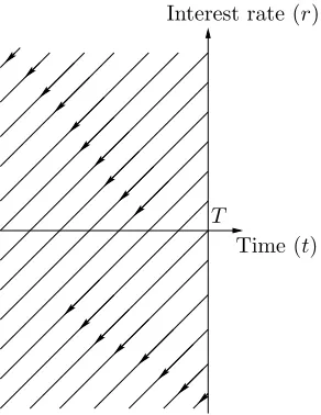
It is possible to find a unique solution to this problem as long as the Cauchy data is not tangent to the characteristics. We can then construct a solution surface which is made up of characteristics which pass through the Cauchy data curve [55].

Since all of the jump and final conditions for our pde will be equations for the contract value in terms of r at a particular time, our Cauchy data will always be parallel to the t-axis in the (r, t) plane, in the direction (0,1). We will therefore be able to solve the pde uniquely as long as the characteristics are never parallel to the

t-axis. The characteristic path is given, according to Equation (2.12), by dr/dt=c, i.e. in the direction (1, c). Consequently, there will be a unique solution as long as c

is finite. Equation (2.4) guarantees that this will always be the case.

The characteristics for the problem are shown in Figure 2.6. They span the whole (r, t) plane fort _≤T and we expect a well-defined solution in this region.

(43)

Interest rate (r)

Time (t)

[image:43.595.254.400.105.294.2]

T

Figure 2.6: Characteristics for the linear problem

Since the Cauchy data is not parallel to the characteristics, we can invert the equations for (r, t) in terms of (s, p) to find (s, p) in terms of (r, t),

s =₋(T ₋t) and p=r+c(T ₋t).

We can then substitute for these into the equation for V to find

V = Λ(r+c(T −t))e−12c(T−t)2−r(T−t).

This solution holds for s_≤0 and _−∞< p <_∞, i.e.

T ₋t _≥0 and _{− ∞}< r+c(T ₋t)<_∞,

which covers the whole (r, t) space for t≤T.

2.5 The characteristics for the nonlinear problem

The characteristics of Equation (2.6) are given by

dt

1 =

dr c(r, Vr)

= dV

rV. (2.13)

The characteristic projections in the (r, t) plane are then

dr

dt =c(r, Vr). (2.14)

We can solve this problem with final condition V(r, T) as long as Vr is nonzero

(44)

by Equation (2.13) and span the solution space. We can then solve along these characteristics, using the final condition as Cauchy data.

If the Cauchy data is discontinuous, then the discontinuity will propagate along a characteristic. This is because any discontinuity in the solution of a hyperbolic partial differential equation must occur across a characteristic. To solve the problem, we simply ‘patch together’ the two classical solutions to the continuous problems either side of the characteristic [54].

However, as soon as there is a point at which Vr = 0, then we do not yet have

a systematic method for constructing the characteristic path through the point. We cannot use Charpit’s method [13] to improve the situation, as the approach does not simplify the dependence of c on Vr into a more tractable form. Instead, we must

examine the various forms in which Vr = 0 can occur, and go back to the modelling

of the problem to explain what happens to the characteristics.

We shall assume that the zero r-derivative occurs in our final data. If this not the case, then we can construct the characteristics and find a solution back until the time when Vr(r, t) = 0 first occurs and then consider this solution as our final data to

proceed further back. To simplify matters, we shall initially only concern ourselves with the local problem around the point where the derivative is zero (i.e. away from the boundaries).

There are essentially two cases to consider:

• A maximum at rT - where Vr(rT, T) = 0, Vr(r−T, T)>0 and Vr(r+T, T)<0.

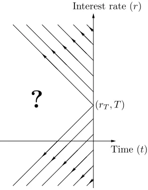
• A minimum at rT - whereVr(rT, T) = 0, Vr(r−T, T)<0 and Vr(rT+, T)>0,

where r−_T and r_T+ are an infinitessimal negative and positive distance away from rT,

respectively.

In the following work, we solve the pde backwards in time, from the final data. All discussion of the evolution of a solution, or the propagation of a turning point refers to the change as time to maturity increases (i.e. backwards in time).

2.5.1 V

r

= 0

at a maximum

We consider the problem with V(r, T) = f(r), where the final data has a maximum at (rT, T). In this case, we have

(45)

Therefore, forr < rT, we havec(r, Vr) = c− and forr > rT, we havec(r, Vr) =c+.

The characteristics are given by

dr dt =c

−_,

for r < rT att =T and by

dr dt =c

+_,

for r > rT att =T.

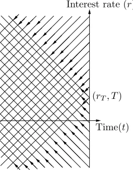
There is a region, shown in Figure 2.7, in which points can be reached by two characteristics. Consequently, there will not be a unique solution in this region. In this and the following figures, we have set c+ ₌ ₋_c− _{to be some positive constant,}

for ease of pictorial representation.

[image:45.595.259.393.311.482.2]

Time(t) (rT, T) Interest rate (r)

Figure 2.7: Multiple characteristics when there is a maximum at (rT, T)

To find a unique solution, we must introduce a shock into the problem. The shock splits the solution space into two regions. In each region, there will only be a single set of characteristics and hence, a unique solution for V. To solve for the position of the shock, we have to go back to the modelling of the problem:

In the worst-case scenario, information (containing the solution) flows from inter-est rates where the contract value is low to those at which it is high. When there is a point at which the contract value has a maximum, then information flows into this point from both sides. This is shown in Figure 2.8, where we have ignored the effect of discounting and examine the evolution of the contract value in a worst-case scenario.

(46)

[image:46.595.259.393.532.700.2]

.

Figure 2.8: Evolution of a maximum without discounting

from one solution to the other, so that the contract value is always as low as possible, must occur such that the solution is continuous. The maximum will always be at the point where the two solutions meet.

Therefore, the condition that we must apply is that the solution for V is continu-ous. This is, in effect, an arbitrage argument, since the formation of a discontinuity would lead to arbitrage opportunities. With this information, we can use the fol-lowing methodology to find the path of the shock. We split the Cauchy data into two sections, with the split at the maximum. We solve the two resulting problems individually. We then equate these two solutions and solve the resulting equation to find a relationship between r and t. This describes the path of the shock. On each side of the shock, we use the solution that came from the Cauchy data to that side. Across the shock, the solution is continuous, by definition. The path of the shock also describes the evolution of the maximum and so the characteristic picture is consistent with this evolution. In Figure 2.9, we show a typical set of characteristics for this problem.

Figure 2.9: Characteristics when there is a maximum at (rT, T) and we introduce a

(47)

2.5.2 The evolution of a maximum

Since the method of solution tracks the maximum, we can study the path that it takes. In the following work, we consider the case wherec+ _and _c− _{are constants and}

examine the local problem around the maximum (i.e. away from the boundaries). The problem we solve is Equation (2.6) with final data

V(r, T) =

f1(r) forr ≤rT

f2(r) forr > rT,

where

df1

dr >0 , df2

dr <0 and f1(rT) =f2(rT),

so that we have a continuous solution. This is shown in Figure 2.10.

1 2

Vr<0

Vr>0

f2(r)

f1(r)

rT

V(r, T)

r

Figure 2.10: The local problem with a maximum at (rT, T)

In region 1, the characteristics are defined by

dt = dr

c− =

dV1

rV1

=ds,

and we have Cauchy data of

Γ1(r, t, V1) = (p, T, f1(p)),

for p < rT. We can solve this to find

V1(r, t) =f1(r+c−(T −t))e−

1

2c−(T−t)2−r(T−t),

for r ≤rT −c−(T −t).

In region 2, the characteristics are defined by

dt = dr

c+ =

dV2

rV2

Uncertain Interest Rate Modelling