A comparison between VEGA 1, 2 and Giotto flybys of comet 1P/Halley: implications for Rosetta

www.ann-geophys.net/32/1441/2014/ doi:10.5194/angeo-32-1441-2014

© Author(s) 2014. CC Attribution 3.0 License.

A comparison between VEGA 1, 2 and Giotto flybys of comet

1P/Halley: implications for Rosetta

M. Volwerk1, K.-H. Glassmeier2, M. Delva1, D. Schmid1, C. Koenders2, I. Richter2, and K. Szegö3

1_{Space Research Institute, Austrian Academy of Sciences, 8042 Graz, Austria} 2_{Institute for Geophysics and Extraterrestrial Physics, TU Braunschweig, Germany}

3_{Wigner Research Centre for Physics, Institute for Particle and Nuclear Physics, Hungarian Academy of Sciences,} Budapest, Hungary

Correspondence to: M. Volwerk ([email protected])

Received: 1 October 2014 – Accepted: 1 November 2014 – Published: 28 November 2014

Abstract. Three flybys of comet 1P/Halley, by VEGA 1, 2

and Giotto, are investigated with respect to the occurrence of mirror mode waves in the cometosheath and field line drap-ing in the magnetic pile-up region around the nucleus. The time interval covered by these flybys is approximately 8 days, which is also the approximate length of an orbit or flyby of Rosetta around comet 67P/Churyumov–Gerasimenko. Thus any significant changes observed around Halley are changes that might occur for Rosetta during one pass of 67P/CG. It is found that the occurrence of mirror mode waves in the come-tosheath is strongly influenced by the dynamical pressure of the solar wind and the outgassing rate of the comet. Field line draping happens in the magnetic pile-up region. Changes in nested draping regions (i.e. regions with differentBx

direc-tions) can occur within a few days, possibly influenced by changes in the outgassing rate of the comet and thereby the conductivity of the cometary ionosphere.

Keywords. Interplanetary physics (interplanetary magnetic

fields; plasma waves and turbulence) – space plasma physics (waves and instabilities)

1 Introduction

In this new era of cometary physics, which started with the arrival of the Rosetta spacecraft (Glassmeier et al., 2007) at comet 67P/Churyumov–Gerasimenko (67P/CG) on 6 Au-gust 2014, it is worthwhile to take another look at previous satellite encounters with comets. Rosetta will orbit around the comet and follow it along its path through perihelion and beyond. Rosetta will thus observe the temporal variations in

the interaction of the outgassing comet with the solar wind magnetoplasma.

In order to simulate Rosetta orbiting 67P/CG and the changes that can be expected in the comet–solar wind in-teraction, three flybys of comet 1P/Halley by VEGA 1, 2 and Giotto are used. These flybys, within a time span of 8 days showed significant differences in the interaction in the plasma data; a similar data set will be generated by the Rosetta Plasma Consortium (RPC, Glassmeier et al., 2007) at 67P/CG.

Two different processes are discussed in this paper, first the presence and generation of mirror mode waves in the cometosheath and then the magnetic field line draping around the nucleus in the magnetic pile-up region.

2 Flybys of comet 1P/Halley by VEGA 1, 2 and Giotto

There have been three close flybys of 1P/Halley by Vega 1, 2 and Giotto, all three within 8 days and along very similar orbits as can be seen in Fig. 1.

The magnetic field data of these flybys are shown in Fig. 2. Note that these data are obtained in shocked solar wind, i.e. within the cometosheath (the region between the bow shock and the ionopause). It is clear from this figure that the flybys show very different conditions around the comet in all components of the magnetic field. The increase of the total magnetic fieldBt during ingress is much more gradual for

VEGA1/2 (red/green) as compared to Giotto (blue). Also, note the different sign ofBx for VEGA1 and VEGA2. For

Giotto, multiple sign changes inBxaround closest approach

Figures −1 −0.8 −0.6 −0.4 −0.2 0 0.2 0.4 0.6 0.8 1

x 106

−1 −0.8 −0.6 −0.4 −0.2 0 0.2 0.4 0.6 0.8 1

x 106

X

CSE [km]

YCSE [km] Giotto VEGA1 VEGA2 −1 −0.5 0 0.5 1

x 105

−1

−0.5

0

0.5

1

x 105

XHSE

YHSE

Fig. 1. The orbits of the three close flybys by Giotto (blue), VEGA 1 (red) and VEGA 2 (green) in CSE coordinates. The dashed line shows the location of the bow shock for the Giotto flyby as a guidance. Note that the bow shock location will differ for the other two flybys. The inset panel shows a zoom-in to clarify the difference in the orbits near the comet.

20

Figure 1. The orbits of the three close flybys by Giotto (blue), VEGA 1 (red) and VEGA 2 (green) in cometocentric–solar–ecliptic (CSE) coordinates. The dashed line shows the location of the bow shock for the Giotto flyby as a guidance. Note that the bow shock location will differ for the other two flybys. The inset panel shows a zoom-in to clarify the difference in the orbits near the comet.

field line draping regions), whereas VEGA1 only shows one, and VEGA2 shows no sign change at all. Thus within a time span of 8 days, the structure of the cometosheath has changed significantly. The magnetic field vector plots of the three fly-bys in the cometocentric–solar–ecliptic (CSE)xyplane, con-taining the dominant magnetic field directions, are shown in Fig. 3. In the CSE coordinate system theX axis points to-wards the Sun, theZaxis is perpendicular to the orbital plane around the Sun (positive towards the north) and theY axis completes the triad.

3 Mirror-mode waves

In order to see how the magnetoplasma changes around the comet the magnetometer data are studied for the pres-ence of mirror-mode (MM) waves within the cometosheath using the magnetic-field-only method presented by Lucek et al. (1999a, b). A sliding window minimum variance anal-ysis (MVA) (Sonnerup and Scheible, 1998) is performed, whereby MMs are identified by the following criteria:

– Angle γ between minimum variance direction and

background magnetic field is larger then 80◦;

– Angle α between maximum variance direction and

background magnetic field is smaller than 20◦;

– The amplitude of the wavesδB/B >0.3.

−50 0 50 100 Bx [nT] −100 0 100 By [nT] −50 0 50 100 Bz [nT] 0 50 100 Bt [nT] −15 −10 −5 0 5 10 15 0 1 2 3 Pb [nPa]

R [105 _km]

Giotto VEGA1 VEGA2

Fig. 2.The magnetic field components in CSE coordinates, total fieldBtand magnetic pressurePbof the three

flybys by Giotto (blue), VEGA 1 (red) and VEGA 2 (green).

−1 0 1

x 106

−1

−0.5

0

0.5

1

x 106

10 nT Giotto

X_CSE [km]

YCSE

[km]

−1 0 1

x 106

−1

−0.5

0

0.5

1

x 106

10 nT VEGA 1

X_CSE [km]

YCSE

[km]

−1 0 1

x 106

−1

−0.5

0

0.5

1

x 106

10 nT VEGA 2

X_CSE [km]

YCSE

[km]

Fig. 3. The orbits of the three close flybys by Giotto (blue), VEGA 1 (red) and VEGA 2 (green) in CSE coordinates with the magnetic field vectors in the CSExy-plane plotted along the spacecraft orbits.

21

Figure 2. The magnetic field components in CSE coordinates,

to-tal fieldBt and magnetic pressurePbof the three flybys by Giotto

(blue), VEGA 1 (red) and VEGA 2 (green).

−50 0 50 100 Bx [nT] −100 0 100 By [nT] −50 0 50 100 Bz [nT] 0 50 100 Bt [nT] −15 −10 −5 0 5 10 15 0 1 2 3 Pb [nPa]

R [105 km]

Giotto VEGA1 VEGA2

Fig. 2.The magnetic field components in CSE coordinates, total fieldBtand magnetic pressurePbof the three

flybys by Giotto (blue), VEGA 1 (red) and VEGA 2 (green).

−1 0 1

x 106

−1

−0.5

0

0.5

1

x 106

10 nT Giotto

XCSE [km]

YCSE

[km]

−1 0 1

x 106

−1

−0.5

0

0.5

1

x 106

10 nT VEGA 1

XCSE [km]

YCSE

[km]

−1 0 1

x 106

−1

−0.5

0

0.5

1

x 106

10 nT VEGA 2

XCSE [km]

YCSE

[km]

Fig. 3.The orbits of the three close flybys by Giotto (blue), VEGA 1 (red) and VEGA 2 (green) in CSE coordinates with the magnetic field vectors in the CSExy-plane plotted along the spacecraft orbits.

21

Figure 3. The orbits of the three close flybys by Giotto (blue), VEGA 1 (red) and VEGA 2 (green) in CSE coordinates with the

magnetic field vectors in the CSExyplane plotted along the

space-craft orbits.

This method has been shown to work well (see e.g. Volw-erk et al., 2008a, b; Schmid et al., 2014; Delva et al., 2014) and in order to improve on the determination of the MMs a lower limit on the goodness of the MVA can be set using the minimumλminand intermediateλinteigenvalues of the MVA matrix through the following:λint/λmin>5. There can be short intervals between MMs in which the criteria as stated above are not fulfilled. However, if that interval is shorter than 20 s the neighbouring MM intervals are considered to be part of one larger interval.

0 5 10 15 20

Bt [nT]

Giotto − 13 March 1986

8 8.5 9 9.5 10

Ne [cm

−3]

23:05 23:06 23:07 23:08

0 20 40 60 80

α

,

γ

[deg]

UT

0 5 10 15 20

Bt [nT]

Giotto − 13 March 1986

9.5 10 10.5

Ne [cm

−3

]

23:21 23:22 23:23 23:24

0 20 40 60 80

α

,

γ

[deg]

UT

Fig. 4. Examples of mirror-mode waves in the Giotto data. Top: Total magnetic field with low-pass filtered

(background) magnetic field as a dashed line; Middle: Electron density; Bottom: Anglesα/γbetween

mini-mum/maximum variance direction with the background magnetic field.

22

Figure 4. Examples of mirror-mode waves in the Giotto data. Top: total magnetic field with low-pass filtered (background) magnetic field as

a dashed line; middle: electron density; bottom: anglesα/γbetween minimum/maximum variance direction with the background magnetic

field.

(Tsurutani et al., 1999). Using VEGA 1 and 2 plasma data Tátrallyay et al. (2000b) have shown the presence of slowed-down solar wind plasma and picked up cometary ions at dis-tances between 1.5 to 0.5 million km from the comet, within the bow shock.

A current discussion on the presence of MMs in planetary magnetosheaths generated by ion temperature anisotropies can be found in Remya et al. (2013) and Tsurutani et al. (2011) gives an overview of MMs in the magnetosheath and heliosheath, and their distinguishing features from magnetic decreases (also known as magnetic holes).

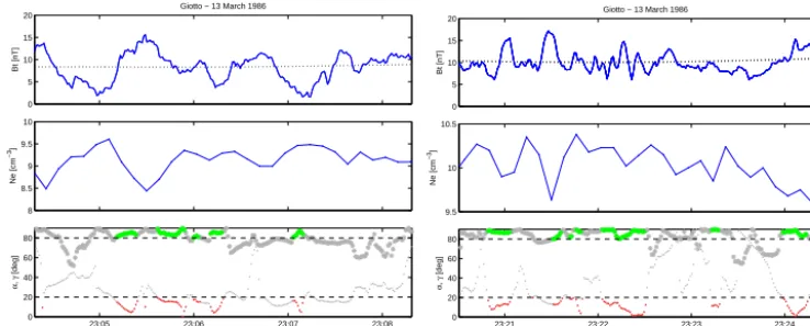
3.1 Giotto

The automated MM search is applied to the Giotto mag-netometer data (Neubauer et al., 1986) at a data resolu-tion of 1 s, over the interval 13 March 1986 19:00 UT un-til 14 March 1986 06:00 UT, which spans the interval that the spacecraft is inside the cometosheath. Two examples of MM wave intervals are shown in Fig. 4, but see also Glass-meier et al. (1993) for further examples. The total magnetic field strength is shown as well as the electron density, indi-cating a good anti-correlation. Also the two anglesαandγ

are displayed; the red/green coloured intervals show where the search criteria are fulfilled.

An overview of all MM events found is given in Fig. 5, where the length, the relative amplitude, the MVA good-ness and the average background magnetic field strength are shown. The red markers show the events for which the MVA goodness is good (λint/λmin>5). The gray box shows the interval of the magnetic pile-up region (MPR) in which no MM events are expected (see e.g. Mazelle et al., 1991; Delva et al., 2014). It is clear that there are many more events be-fore the MPR than after, indeed the last 3 h do not show any activity and are therefore omitted in the figure.

To make the distribution of the MM events clearer, his-tograms for ingress (Fig. 6 top left) and egress (Fig. 6 top

18:000 21:00 00:00 03:00

20 40 60 80

UT

length [s]

MM length

18:000 21:00 00:00 03:00

10 20 30 40 50 60

UT λint

/

λmin

MM goodness

18:000 21:00 00:00 03:00

5 10 15 20

UT

∆

B/B

MM strength

18:000 21:00 00:00 03:00

5 10 15 20

UT

|B| [nT]

Average field strength

Fig. 5.Overview of all the time intervals with MMs for the Giotto flyby. Shown are the length of the interval, the goodness of the MVA, the strength of the MMs and the average background field strength. The red circles show for which MMs the MVA goodness is greater than 5. The gray-shaded area is the magnetic pile-up region in which no MMs are expected.

23

Figure 5. Overview of all the time intervals with MMs for the Giotto flyby. Shown are the length of the interval, the goodness of the MVA, the strength of the MMs and the average background field strength. The magenta circles show for which MMs the MVA good-ness is greater than 5. The gray-shaded area is the magnetic pile-up region in which no MMs are expected.

right) show the number of events binned by the number of sequential sliding windows which means that the total length of the MM interval in seconds is 30 s longer. From the his-tograms it is clear that during ingress there are many more events than at egress. This is partially caused by the shorter period in the cometosheath after exiting the MPR, but that cannot explain the total discrepancy. Therefore, there have to be different reasons for this, which will be discussed below.

3.2 VEGA 1

0 20 40 60 80 100 0

10 20 30 40 50

# windows mm interval

# comb. events

Ingress

0 20 40 60 80 100 0

10 20 30 40 50

# windows mm interval

# comb. events

Egress

0 20 40 60 80 100 0

10 20 30 40 50

# windows mm interval

# comb. events

Ingress

0 20 40 60 80 100 0

10 20 30 40 50

# windows mm interval

# comb. events

Egress

0 20 40 60 80 100 0

10 20 30 40 50

# windows mm interval

# raw events

Ingress

Fig. 6.Histograms of the number of time windows in which MMs were observed per event at ingress (left) and egress (right) for Giotto (blue), VEGA 1 (red) and VEGA 2 (green). To obtain the length of the MM interval the length of the window, 30 s, should be added to the size of the bin. For VEGA 2 the requirement on the amplitude∆B/B >0.3has been dropped, and thus the number of events is increased.

24

Figure 6. Histograms of the number of time windows in which MMs were observed per event at ingress (left) and egress (right) for Giotto (blue), VEGA 1 (red) and VEGA 2 (green). To obtain the length of the MM interval the length of the window, 30 s, should be added to the size of the bin. For VEGA 2 the requirement on the

amplitude1B/B >0.3 has been dropped, and thus the number of

events is increased.

1986) at a resolution of 1 s, between∼04:30 and∼08:30 UT are searched for MM waves. An example of an MM interval is shown in Fig. 7, and an overview of all events found is shown in Fig. 8. In this case there are fewer events before the MPR than after, even though the egress time interval is shorter.

Figure 6 middle panels show histograms of the duration of the MM intervals, which shows an almost smooth distri-bution of MM interval lengths. Apart from there being less events compared to the Giotto flyby, there are slightly less events during ingress than egress, although there is not a great difference in total number of events.

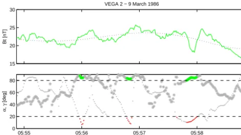
3.3 VEGA 2

The VEGA 2 flyby occurred on 9 March 1986, 3 days af-ter VEGA 1 and 5 days before Giotto. Here the magne-tometer data were used at 1 s resolution for the interval

∼04:15–∼07:20 UT, i.e. up until closest approach, after which the sensor was saturated and no longer useful for data evaluation. An example of a MM interval is shown in Fig. 9,

0 5 10 15 20 25

Bt [nT]

VEGA 1 − 6 March 1986

08:19 08:20 08:21 08:22

0 20 40 60 80

α

,

γ

[deg]

UT

Fig. 7.Example of an MM interval in the VEGA 1 data, in similar format as Fig. 4.

25

Figure 7. Example of an MM interval in the VEGA 1 data, in simi-lar format as Fig. 4.

03:000 06:00 09:00

20 40 60 80

UT

length [s]

MM length

03:000 06:00 09:00

5 10 15 20 25 30

UT λint

/

λmin

MM goodness

03:000 06:00 09:00

1 2 3 4

UT

∆

B/B

MM strength

03:000 06:00 09:00

10 20 30 40 50 60

UT

|B| [nT]

Average field strength

Fig. 8.Overview of all MM intervals for the VEGA 1 flyby, in similar format as Fig. 5.

26

Figure 8. Overview of all MM intervals for the VEGA 1 flyby, in similar format as Fig. 5.

where possibly only the last interval at 05:58 UT is a true MM. Note that in this case the amplitudes 1B/B of the MMs, as shown in Fig. 10 is much smaller than in the other two flybys discussed above. The requirement on the

ampli-tude1B/B >0.3 was relaxed for VEGA 2 in order to find

more events. For completeness the distribution of the MMs is shown in Fig. 6, however this cannot be compared directly with the other two histograms shown above.

3.4 MM determination: a recap

15 20 25 30

Bt [nT]

VEGA 2 − 9 March 1986

05:55 05:56 05:57 05:58

0 20 40 60 80

α

,

γ

[deg]

UT

Fig. 9.Example of an MM interval in the VEGA 2 data, in similar format as Fig. 4.

27

Figure 9. Example of an MM interval in the VEGA 2 data, in simi-lar format as Fig. 4.

wave activity, with a strong number-preference for the in-bound leg of the flyby.

The overview of the magnetic fields, see Fig. 2, shows that apart from the difference in the direction of Bx, the

come-tosheath total magnetic fieldBtremains constant over a large

distance for Giotto, whereas the magnetic field for the VEGA flybys show more variations and a slow but gradual increase towards closest approach.

Figure 3 shows the vector plots of the magnetic field along the orbits of the three spacecraft in the CSExy plane, low-pass filtered for periods longer than 20 min. This shows that on time scales longer than 20 min the magnetic field strongly rotates in thexyplane for Giotto, with mainlyBxvariations,

whereas it remains rather constant for VEGA 1 with major negative By component and VEGA 2 with major positive Bx component. This probably means that a constant

direc-tion of the magnetic field is not a major player in the creadirec-tion of the MMs.

4 Sources of changes in the cometosheath

The outgassing comet is embedded in the solar wind, and therewith two sources for changes in the cometosheath are already found. An increased dynamic pressure of the solar wind will make the cometosheath shrink; on the other hand an increase in outgassing will extend the cometosheath; both will also influence the magnetic field structure.

4.1 Solar wind

Changes in the solar wind, such as the interplanetary mag-netic field (IMF) direction or dynamic pressure, will lead to a different interaction with the comet. It is already clear from Fig. 3 that there seem to be nested draping regions around 1P/Halley during the Giotto flyby (Raeder et al., 1987), whereas the draping pattern for VEGA 1 and 2 seem to be rather constant if differently directed. In order to see the behaviour of the solar wind during the flybys, the aver-age values for the IMF are shown in Table 1.

04:000 05:00 06:00 07:00

5 10 15 20 25 30 35

UT

length [s]

MM length

04:000 05:00 06:00 07:00

5 10 15 20

UT λint

/

λmin

MM goodness

04:000 05:00 06:00 07:00

0.1 0.2 0.3 0.4 0.5 0.6 0.7

UT

∆

B/B

MM strength

04:00 05:00 06:00 07:00

10 15 20 25 30 35 40

UT

|B| [nT]

Average field strength

Fig. 10.Overview of all MM intervals for the VEGA 2 flyby, in similar format as Fig. 5.

28

Figure 10. Overview of all MM intervals for the VEGA 2 flyby, in similar format as Fig. 5.

For the Giotto flyby the IMF direction changes signifi-cantly between before entering the cometosheath and after exiting. Unfortunately, there are no plasma data available af-ter closest approach. Similarly, for VEGA 1 the IMF changes drastically between inbound and outbound as is evident by the sign changes of bothBx andBy. For VEGA 2 there is

only inbound information for the magnetic field.

It is clear that 1P/Halley is in a completely different solar wind during the flybys of VEGA 1/2 as compared with the Giotto flyby, as tabulated in Table 1. The dynamic pressure is 4 to 5 times larger in the former. This results in a very different magnetic pressure in the cometosheath, which can be seen in Fig. 2 bottom panel, for VEGA 1 and VEGA 2 the magnetic pressurePbis a factor of 5 and 4 greater than for Giotto, during ingress.

4.2 Cometary outgassing

The outgassing of comets is not a continuous phenomenon, and can vary strongly during the perihelion passage; see e.g. Silva and Mirabel (1988) for outbursts of comet 1P/Halley; Grothues (1996) for outbursts of comet P/Faye 1991 XXI; Biver et al. (2007) for outbursts of comet 9P/Tempel 1; and Meech et al. (2013) for outbursts of comet C/2012 S1 ISON.

Observations in the visual (Green and Morris, 1987) and in the infrared (Gehrz et al., 2005) have shown that the bright-ness of comet 1P/Halley in general followed the expected light curve, however, there were strong short time scale (hours, days) variations in the brightness of the comet. These enhancements are connected to bursts in the outgassing of the comet.

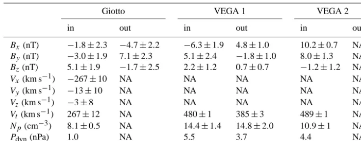
Table 1. 30 min averages of the solar wind parameters before and after bow shock crossing.

Giotto VEGA 1 VEGA 2

in out in out in out

Bx(nT) −1.8±2.3 −4.7±2.2 −6.3±1.9 4.8±1.0 10.2±0.7 NA

By(nT) −3.0±1.9 7.1±2.3 5.1±2.4 −1.8±1.0 8.0±1.3 NA

Bz(nT) 5.1±1.9 −1.7±2.5 2.2±1.2 0.7±0.7 −1.2±1.2 NA

Vx(km s−1) −267±10 NA NA NA NA NA

Vy(km s−1) −13±10 NA NA NA NA NA

Vz(km s−1) −3±8 NA NA NA NA NA

Vt(km s−1) 267±12 NA 480±1 385±3 489±1 NA

Np(cm−3) 8.1±0.5 NA 14.4±1.4 14.8±2.0 10.9±1 NA

Pdyn(nPa) 1.0 NA 5.5 3.7 4.4 NA

for the VEGA 1 encounter was much higher than for the VEGA 2 encounter.

Gehrz et al. (2005) used the Lyαmeasurement from the Pioneer Venus UV spectrometer (Stewart, 1987) and the OH measurements from the IUE (Feldman et al., 1987) of comet 1P/Halley to obtain the water production rate. The flybys of the three spacecraft discussed in the current paper is cov-ered by the period over which the activity of the comet was monitored, shown in Fig. 8 of Feldman et al. (1987). It was found that the water production had a strong de-crease from∼1.5×1030 to∼5.0×1029molecules s−1 on 7 March. This means that the VEGA 1 flyby was during high-rate outgassing, whereas the VEGA 2 and Giotto fly-bys were during low-rate outgassing, in good agreement with Tátrallyay et al. (2000b).

4.3 Suppression of MMs

The mirror mode wave is generated by freshly picked up ions near the comet which will create a ring distribution in ve-locity space with parallel temperature Tk smaller than

per-pendicular temperatureT⊥. The instability criterion for MM

waves is given by the inequality (Hasegawa, 1969):

1+β⊥

1−T⊥ Tk

<0, (1)

whereβ⊥=(nkBT⊥)/(B2/2µ0)is the so-called perpendic-ular plasma-β. Equation (1) can be rearranged into

_T

⊥

Tk

−1

> β_⊥−1= B

2

2µ0nkBT⊥

, (2)

which indicates that for strong fields less MM are expected. This leads to an understanding why there are such strong dif-ferences in MM occurrence between the three flybys.

– During the VEGA 1 flyby, there was strong outgassing,

i.e. strong pickup of freshly ionised water. This hap-pened in a very strong magnetic field, with an average

magnetic pressure of∼0.15 nPa during ingress. The so-lar wind is slowed down significantly (Tátrallyay et al., 2000b). Apparently, the energy density in the picked-up ions, determined by density and pick-picked-up velocity, is large enough to increaseβ⊥and hence fulfill the

insta-bility criterion in Eq. (2).

– During the VEGA 2 flyby, the outgassing dropped by a

factor of 3, hence the pickup of freshly ionised water de-creased as well, the solar wind slowed down similarly to the VEGA 1 flyby. The magnetic pressure, however, in the cometosheath remained at a high level,∼0.12 nPa. In this case the energy density in the picked-up ions is not enough to increaseβ⊥sufficiently. This leads to a

lack of MM structures.

– During the Giotto flyby the outgassing of the comet

re-mained at a low level, however, also the magnetic pres-sure in the cometosheath was significantly reduced to

∼0.03 nPa. The solar wind velocity is still low, compa-rable to the VEGA flybys (Glassmeier et al., 1993). The reduction of the magnetic pressure decreasedβ⊥again

sufficiently to fulfill the instability criterion of Eq. (2). With the lowered magnetic pressure it is easier to gener-ate MMs, thus the increased number of events compared with VEGA 1.

−50 0 50 100

Bx [nT]

Giotto − 13 March 1986

−50 0 50 100

By [nT]

−50 0 50 100

Bz [nT]

0 50 100 150

Bt [nT]

23:30 00:00 00:30 01:00

0 0.5 1

Pb [nPa]

UT

0 10 20

−20 −15 −10 −5 0 5 10

y =−1.38x+6.55 r

c =−0.70 ns =451; 1 av /(1 s) 23:38:00 to 23:45:59

Bx [nT]

Brad [nT]

0 10 20

−30 −25 −20 −15 −10 −5 0

y =−1.02x−3.37 r

c =−0.89 ns =765; 1 av /(1 s) 00:41:00 to 00:55:59

Bx [nT]

Brad [nT]

10 20 30 40 50 60

0 10 20 30 40

y =+1.00x−18.21 r

c =+0.92 ns =197; 1 av /(1 s) 00:04:30 to 00:07:59

Bx [nT]

Brad [nT]

1 2 3 4 5 6 7 8 9 10

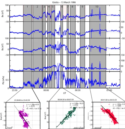
„bad“ „peculiar“ „good“

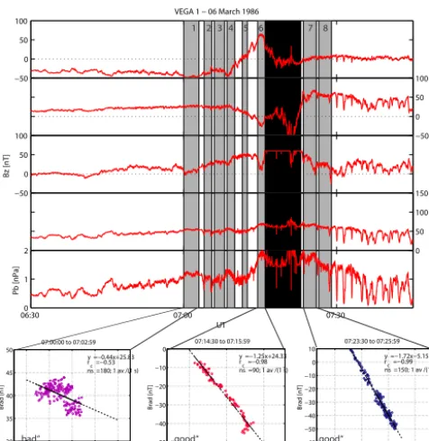
Fig. 11.Top panel: The magnetic field data from Giotto with the ten intervals for which field line draping was studies marked in gray. The red dotted lines show the boundaries between differently draped field as determined by Raeder et al. (1987). Bottom panels: Field line draping fits, according to Eg. (3) for three intervals: a “bad” fit with|rc| ≤0.8; a “peculiar” fit with positive slopeAand a “good” fit withrc≥0.8.

29

Figure 11. Top panel: the magnetic field data from Giotto with the 10 intervals for which field line draping was studies marked in gray. The red dotted lines show the boundaries between differently draped field as determined by Raeder et al. (1987). Bottom panels: field line draping fits, according to Eq. (3) for three intervals: a bad fit with|rc| ≤0.8; a peculiar fit with positive slopeAand a good fit with rc≥0.8.

5 Magnetic field line draping

Magnetic field line draping, i.e. the hanging up of the IMF in the conducting ionosphere around the cometary nucleus was first proposed by Alfvén (1957) for the mechanism by which cometary ion tails are formed. The “far end” of the field line is transported by the solar wind, whereas the part near the comet is slowed down by the conducting layer. Thus the field wraps around the nucleus, bending from the IMF direction into theXCSEdirection.

Using the Giotto data at comet 1P/Halley, Raeder et al. (1987) used vector plots of the magnetic field along the trajectory of the spacecraft, similar to Fig. 3, and showed that there were many directional changes in the draping pattern. Looking at the “nesting” of these directional changes, they were able to connect these changes on the ingress part with those on the egress leg of the orbit. This showed that there was a pile-up of old IMF layers around the comet. A comparison of field line draping around comet 21P/Giacobini–Zinner and Venus, creating a magnetotail, has been studied by McComas et al. (1987) using ICE and PVO data from flybys through the respective (induced) magnetotails.

Israelevich et al. (1994) introduced a method to identify regions where the magnetic field has a draped-like structure.

B1

Bx,imf Brad

B2

Bx,imf Brad

Fig. 12.Magnetic field draping around a comet and field projections at two different locations showing that the radial projection of the draped magnetic field changes direction for “over-draped” field lines.

30

Figure 12. Magnetic field draping around a comet and field projec-tions at two different locaprojec-tions showing that the radial projection of the draped magnetic field changes direction for “over-draped” field lines.

The magnetic field data are projected on a pre-encounter solar wind coordinate system, whereXIMFis along the solar wind velocity,YIMFis given by the cross product of the so-lar wind velocity and the IMF andZIMFcompletes the triad. The encounter magnetic field is projected onto this coordi-nate system producingBX,IMFand a transverseBT,IMF. The latter is projected onto the radial direction from the comet to the spacecraft, producingBrad, see Fig. 12. In the case of field line draping there is a linear dependence:

Brad=ABX,IMF+C. (3)

Indeed, Israelevich et al. (1994) found that for the Giotto flyby at both ingress and egress, close to the comet there is a linear dependence. They show that the draping is a feature of the MPR, whereas in the cometosheath the field is too turbulent to show any such feature. Similarly, Delva et al. (2014) have shown that for the VEGA 1 en-counter at comet 1P/Halley there is field line draping within the MPR, but no such feature outside.

5.1 A more detailed look

Israelevich et al. (1994) used the full MPR, with exclusion of closest approach where the spacecraft entered the diamag-netic cavity, to determine the relationship betweenBradand

BX,IMF. In this section a closer look at the data is taken; shorter time intervals related to the different draping regions that were determined by Raeder et al. (1987).

−50 0 50 100

VEGA 1 − 06 March 1986

Bx [nT]

−50 0 50 100

By [nT]

−50 0 50 100

Bz [nT]

0 50 100 150

Bt [nT]

06:300 07:00 07:30

1 2

UT

Pb [nPa]

1 2 3 4 5 6 7 8

−40 −35 −30 −25 −20

30 35 40 45 50

y =−0.44x+25.83 r

c =−0.53 ns =180; 1 av /(1 s) 07:00:00 to 07:02:59

Bx [nT]

Brad [nT]

20 40 60

−50 −40 −30 −20 −10 0

y =−1.25x+24.33 rc =−0.98 ns =90; 1 av /(1 s) 07:14:30 to 07:15:59

Bx [nT]

Brad [nT]

−20 0 20 40

−60 −50 −40 −30 −20 −10 0 10

y =−1.72x−5.15 rc =−0.99 ns =150; 1 av /(1 s) 07:23:30 to 07:25:59

Bx [nT]

Brad [nT]

„bad“ „good“ „good“

Fig. 13.Top panel: The magnetic field data from VEGA 1 with the eight intervals for which field line draping was studies marked in gray. The black area shows the region where the magetometer was saturated and which was excluded from analysis. Bottom panels: Field line draping fits, according to Eg. (3) for three intervals: a “bad” fit with_|rc| ≤0.8; and two “good” fit with|rc| ≥0.8pre- and post-closest approach respectively.

31

Figure 13. Top panel: the magnetic field data from VEGA 1 with the eight intervals for which field line draping was studies marked in gray. The black area shows the region where the magnetometer was saturated and which was excluded from analysis. Bottom panels: field line draping fits, according to Eq. (3) for three intervals: a bad fit with|rc| ≤0.8; and two good fits with|rc| ≥0.8 pre- and post-closest approach, respectively.

the boundaries for the draping that were determined by Raeder et al. (1987), marked by dotted red lines. The results of the fit given by Eq. (3) are shown in Table 2. Clearly, not all fits are good as is evident from the correlation coefficient, rc, being small. Three examples of “bad”, a “peculiar” and a “good” fits are shown in Fig. 11.

It is clear from the fit results in Table 2 that there is an anti-correlation betweenBradandBX,IMF, something also found by other studies (Delva et al., 2014) and at e.g. Venus and Mars which have a cometary-like interaction with the solar wind (Bertucci et al., 2003a, b). However, this current study finds that near closest approach there is a positive slope of the fit, as seen for intervals 4, 5 and 6 in Table 2. This indicates that the magnetic field is over-draped, bending towards the axis of the tail as was observed e.g. at Venus (Zhang et al., 2010). A schematic of the change betweenBradpositive and negative can be seen in Fig. 12, where forB1it is seen that

Bradis projected outward, whereas forB2it is found thatBrad is projected inward. This phenomenon of positive correlation can only happen on the “night-side” of the comet and because of the orbit of the spacecraft, seen in Fig. 1, such a region is not crossed during egress. Speculatively, there could even be the possibility that a closed loop around the nucleus is created by a tail reconnection event.

Table 2. Magnetic field line draping fit results

Brad=ABX,IMF+C

Giotto (13 March 1986)

no. time fit rc points

1 23:38–23:46 −1.38X+6.55 −0.70 451

2 23:47–2353 −0.82X+5.42 −0.82 479

3 23:56:30–23:59 0.26X+6.12 0.36 141

4 00:01–00:03:30 0.58X−4.99 0.7 141

5 00:04:30–00:08 1.00X−18.21 0.92 197

6 00:13:30–00:15:30 −1.00X−2.16 −0.89 82

7 00:19:30–00:21 −1.11X−6.74 −0.64 74

8 00:22:30–00:27:30 −0.86X+2.70 −0.82 258

9 00:32–00:36:30 −0.81X+8.38 −0.78 247

10 00:41–00:56 −1.02X−3.37 −0.89 765

VEGA 1 (6 March 1986)

1 07:00–07:03 −0.44X+25.83 −0.53 180

2 07:04–07:05:30 −0.69X+17.46 −0.633 68

3 07:06–07:08 −0.77X+15.58 −0.76 120

4 07:08:30–07:10 −0.64X+19.63 −0.82 90

5 07:11:30–07:12:30 −0.89X+14.80 −0.94 60

6 07:14:30–07:16 −1.25X+24.33 −0.98 90

7 07:23:30–07:26 −1.72X−5.15 −0.99 150

8 07:26:30–07:29 −1.36X−12.36 −0.82 150

VEGA 2 (9 March 1986)

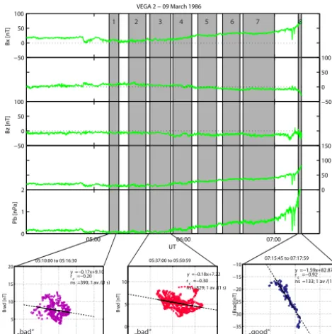
1 05:10–05:16:30 −0.17X+9.10 −0.20 390

2 05:23–05:25 −0.06X+9.51 −0.04 681

3 05:37–05:51 −0.18X+7.22 −0.30 829

4 05:52:30–06:05 −0.68X+14.86 −0.57 744

5 06:09–06:21 −0.24X+3.54 −0.20 720

6 06:25:30–06:37 −0.54X+8.69 −0.58 690

7 06:39–07:00 −0.37X+4.35 −0.37 1246

8 07:15:45–07:18 −1.59X+82.87 −0.92 133

At VEGA 1 the same study is performed (see also Delva et al., 2014) and the chosen intervals can be found in Table 2 and seen in Fig. 13. The interval in black is where the mag-netometer saturated, which is not taken into consideration for data analysis. Only near closest approach inside the MPR, intervals 5, 6 7 and 8, there is a very clean draping signa-ture, with high values of the correlation coefficient rc. Fur-ther away from the comet in the cometosheath the correla-tion is bad with low values of the rc (see Table 2). This is in agreement with the earlier statement that the turbulence in the cometosheath dominates the draping pattern. The same holds for the draping during the VEGA 2 flyby, shown in Fig. 14. Only the short interval 8, before closest approach shows a clear field line draping signature.

5.2 Interpretation of draping fit

0 5 10 15 20 0

5 10 15 20

y =−0.17x+9.10 rc =−0.20 ns =390; 1 av /(1 s) 05:10:00 to 05:16:30

Bx [nT]

Brad [nT]

0 5 10 15 20

0 5 10

y =−0.18x+7.22 rc =−0.30 ns =829; 1 av /(1 s) 05:37:00 to 05:50:59

Bx [nT]

Brad [nT]

50 60 70 80

−40 −35 −30 −25 −20 −15 −10

y =−1.59x+82.87 r

c =−0.92 ns =133; 1 av /(1 s) 07:15:45 to 07:17:59

Bx [nT]

Brad [nT]

−50 0 50 100

Bx [nT]

VEGA 2 − 09 March 1986

−50 0 50 100

By [nT]

−50 0 50 100

Bz [nT]

0 50 100 150

Bt [nT]

05:00 06:00 07:00

0 1 2

Pb [nPa]

UT

1 2 3 4 5 6 7 8

„bad“ „bad“ „good“

Fig. 14.Top panel: The magnetic field data from VEGA 2 with the seven intervals for which field line draping was studies marked in gray. Bottom panels: Field line draping fits, according to Eq. (3) for three intervals: two “bad” fit with|rc| ≤0.8; and the only “good” fit with|rc| ≥0.8.

32

Figure 14. Top panel: the magnetic field data from VEGA 2 with the seven intervals for which field line draping was studies marked in gray. Bottom panels: field line draping fits, according to Eq. (3) for three intervals: two bad fits with|rc| ≤0.8; and the only good fit with|rc| ≥0.8.

into the direction towards the axis of the cometary ion tail as explained above and in Fig. 12.

However, it is also seen that the slope of the draping fit for good fits, i.e. |rc| ≥0.8 (see Table 2), varies be-tween−0.64≤A≤ −1.72 as the spacecraft move past the cometary nucleus. In Fig. 15 the slope is plotted as a function of radial distance from the comet. There seems to be a weak trend for the slope to increase with decreasing distance to the comet. Also the offsetCvaries strongly,−18≤C≤82, but that is a direct consequence of the fact thatBradis the projec-tion ofBtranson the radial direction and thusBradandBX,IMF do not add up toB.

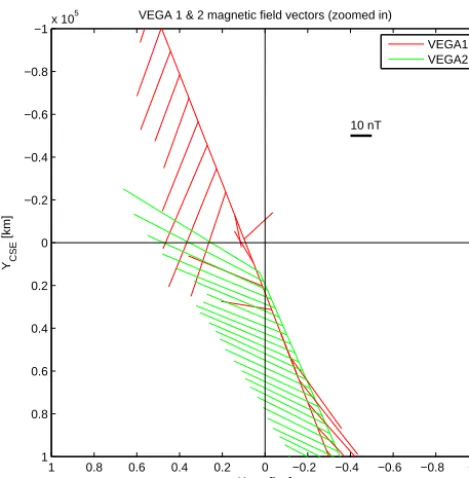
There is evidence of only little nesting of different draping regions for VEGA 1 (Riedler et al., 1986), compared to what has been seen during the Giotto flyby (Raeder et al., 1987). Near closest approach before the saturation, during intervals 4, 5 and 6, there is a good draping fit. However, from Fig. 13 it is clear that 4 and 6 have oppositely directedBx, with

inter-val 5 having basicallyBx=0. However, for the VEGA 2

fly-bly there is no change in the direction of the draped magnetic field. This means that either VEGA 2 did not approach the cometary nucleus close enough to actually penetrate deeply into the pile-up region, or the changes in the environment between the two flybys caused the nested fields to dissipate. Zooming in on the vector plots of the two flybys, as shown in Fig. 16, shows that VEGA 2 is clearly entering a region where there was already a directional change for VEGA 1.

0 2 4 6 8 10 12 14 16 18 20

0.8 1 1.2 1.4 1.6 1.8 2

distance from comet (104 km)

slope |A|

Giotto VEGA 1 VEGA 2

Fig. 15.The slope|A|of the draping fit as given in Eq. (3) as a function of radial distance to the comet.

33

Figure 15. The slope|A|of the draping fit as given in Eq. (3) as a

function of radial distance to the comet.

The solar wind dynamic pressure remained basically the same for VEGA 1 and 2, however, the outgassing of 1P/Halley was strongly reduced. This reduction will lead to less ionisation which will have two effects: (1) less ion pick up by the solar wind IMF and thus less slow down; and (2) a lesser conductivity of the ionosphere and thus less hang-up of the field lines. Both effects will lead to a faster transport of the “old” magnetic field away from the pile-up region.

With the lesser solar wind dynamic pressure during the Giotto flyby, lesser pick up can significantly decelerate the solar wind in the cometosheath, as was observed by e.g. Glassmeier et al. (1993). Checking the solar wind IMF the day before the encounter of Giotto (12 March 1986, not shown), reveals several directional changes in all three com-ponents of the magnetic field. Convection of these structures and subsequent hanging-up in the MPR with only slow dif-fusion will lead to the observed nested draping.

6 Connection between mirror mode waves

and field line draping

Mirror mode waves, as explained above, are generated by a temperature asymmetry with an instability criterion given by Eq. (1). The temperature asymmetry can be generated by heating at the quasi-parallel bow shock (see e.g. Zwan and Wolf, 1976) or by magnetic field line draping and pile-up (see e.g. Midgley and Davis Jr., 1963; Zwan and Wolf, 1976; Tsurutani et al., 1982; Volwerk et al., 2008b).

−1 −0.8 −0.6 −0.4 −0.2 0 0.2 0.4 0.6 0.8 1

x 105 −1

−0.8

−0.6

−0.4

−0.2

0

0.2

0.4

0.6

0.8

1 x 105

10 nT VEGA 1 & 2 magnetic field vectors (zoomed in)

X CSE [km]

YCSE

[km]

VEGA1 VEGA2

Fig. 16.Vector plots of the low-pass filtered magnetic field for VEGA 1 (red) and 2 (green), zoomed in on the inner 10000 km around the cometary nucleus. VEGA 2 enters well into the region where VEGA 1 shows changes in the sign ofBx, but VEGA 2 shows only one sign ofBx.

34

Figure 16. Vector plots of the low-pass filtered magnetic field for VEGA 1 (red) and 2 (green), zoomed in on the inner 10 000 km around the cometary nucleus. VEGA 2 enters well into the region

where VEGA 1 shows changes in the sign ofBx, but VEGA 2 shows

only one sign ofBx.

magnetic field strength increases. The first adiabatic invari-ant µ=mv2_⊥/2B makes that with increasing field strength the perpendicular temperature of the ions increases, thereby increasing the temperature asymmetry and augmenting the MM instability.

It has been shown by Schmid et al. (2014) that MMs are created by local pick up of ions near the cometary nucleus. At comet 1P/Halley the cometopause, the boundary that sep-arates the region of fast flowing solar wind protons domi-nated plasma from the more slowly flowing cometary ions dominated plasma, was located at∼1.6×105km from the nucleus (Gringauz et al., 1986). The first MM encountered by Giotto was measured at∼(−0.3,−1.1.−0.1)×106km, well away from the cometopause, which means the picked-up cometary ions will also experience this energisation, and thus more and stronger events should be expected near the MPR.

Figure 5 shows the Giotto events, where the MPR is grayed-out. There is a clustering of more events at the MPR, but no clear increase in strength. Inside the MPR events are found which are comparable to those outside the MPR. However, Mazelle et al. (1991) have shown that the waves outside and inside the MPB are rather different, where out-side the MPB the electron density variations and the mag-netic field variations are in anti-phase (as expected for MMs) and inside the MPB these are in phase and are identified as a fast magnetoacoustic waves (see also Glassmeier et al.,

1 2 3 4

Dist Sun [AU]

Numerical simulation solar wind−67P/CP interaction

0 20 40 60 80 100

B [nT]

B_imf

Bpileup

0 2 4 6 8 10

N [cm

−3]

0 2000 4000 6000 8000 10000

Dist. [km]

Dist. bow shock Dist. Ionopause

2014/09/01 2014/12/01 2015/03/01 2015/06/01 2015/09/01 2015/12/01

0 2000 4000 6000 8000 10000

L [km]

date Pickup cycloid pileup

Fig. 17. The time development of various parameters around comet 67P/CG obtained from the model by Koenders et al. (2013): The distance comet-Sun; the magnetic field strength of the IMF and the pile-up region; the ion density; the distance of the bow shock and the ionopause from the comet; the radius of the pick-up cycloid at the pile-up boundary. The gray-shaded area shows the interval during which the cometosheath has a size greater than 2 ion gyro radii.

35

Figure 17. The time development of various parameters around comet 67P/CG obtained from the model by Koenders et al. (2013): the distance comet–Sun; the magnetic field strength of the IMF and the pile-up region; the ion density; the distance of the bow shock and the ionopause from the comet; the radius of the pick-up cycloid at the pile-up boundary. The gray-shaded area shows the interval during which the cometosheath has a size greater than 2 ion gyro radii.

1993). Indeed, it seems that the magnetic pile-up bound-ary (MPB), where the strong increase of the magnetic field strength starts, separates two plasmas with different qualities. Neubauer (1987) showed that he MPB can be described by as a rotational discontinuity with strongly differing plasma anisotropies on either side. Studying suprathermal electrons, Mazelle et al. (1989) showed that there was a clear plasma discontinuity at the MPB.

7 Implications for Rosetta

expected at 67P/CG with respect to the ever changing inter-action of the outgassing comet and the dynamic solar wind.

67P/CG is a weakly outgassing comet, and the interac-tion region around the nucleus is only slowly growing, as shown in Koenders et al. (2013, Fig. 11). Recently, Rubin et al. (2014) have used both a multifluid-MHD and a hybrid code to model the interaction of the solar wind with a weakly outgassing comet. The magnetic pile-up region is expected to be fully developed in May 2015 and the bow shock is not expected to appear until July 2015. This means that the mag-netic field line draping can studied from rather early on in the mission during the escort phase. However, for the mirror mode waves the situation is different as they will develop out-side the MPR but inout-side the bow shock, in the cometosheath. The expected global morphology of the interaction region of the solar wind with the outgassing 67P/CG has recently been discussed by Mendis and Horányi (2014).

Figure 17 shows the time development of various param-eters: the distance of the 67P/CG to the sun, the solar wind and pile-up magnetic field strength, the density, the distance of the bow shock and the ionopause and the pick-up ion cycloid at the pile-up boundary, as taken from the simula-tions by Koenders et al. (2013). From measurements at comet 1P/Halley it was found that the size of the water mirror mode waves was on the order of 1 to 2 ion gyro radii (Schmid et al., 2014), therefore it stands to reason that the size of the come-tosheath should at least be 2 ion gyro radii. In Fig. 17 the gray bar shows the region in which the gyro radius is less than half the bow shock distance. This indicates that there will be only a small time window in which these waves can develop from ion pick up near the comet.

8 Conclusions

The opportune flybys of comet 1P/Halley by three space-craft over a time span of 8 days have shown how strongly the interaction of an outgassing comet with the solar wind can change over a time interval which is similar to a Rosetta flyby of/orbit around comet 67P/Churyumov-Gerasimenko. Changes in the dynamic pressure of the solar wind will have influence on the generation of mirror-mode waves in the cometosheath, as well as a change in the outgassing rate of the comet. Increased solar wind dynamic pressure will com-press the magnetosheath and inhibit MM growth, whereas in-creased outgassing will enhance ion pick up and assist MM growth.

Magnetic field line draping and pile-up near the cometary nucleus leads to nested draping, i.e. regions of differently di-rected magnetic field in the MPR. The change in outgassing rate, and therewith the change in ionisation and ionospheric conductivity leads to a disappearance of the nested structures (between VEGA 1 and VEGA 2), whereafter a new nested structure is build up (between VEGA 2 and Giotto).

Although comet 1P/Halley was up to 2 orders of magni-tude stronger in outgassing than 67P/CG will be, the basic physical processes will remain the same. The yield of the three 1P/Halley flybys discussed in this paper for the Rosetta mission is to show that the cometary environment can change quickly and well within the planned duration of the Rosetta flybys.

Acknowledgements. The authors would like to acknowledge the

PDS/PPI for the Giotto and VEGA1/2 magnetometer data. The work of K.-H. Glassmeier, I. Richter and C. Koenders was finan-cially supported by the German Bundesministerium für Wirtschaft und Energie and the Deutsches Zentrum für Luft- und Raumfahrt under contract 50 QP 1001 for Rosetta. D. Schmid acknowledges support by the Austrian Science Foundation (FWF) under contract P25257-N27.

Topical Editor L. Blomberg thanks two anonymous referees for their help in evaluating this paper.

References

Alfvén, H.: On the theory of comet tails, Tellus, 9, 92–96, 1957. Bertucci, C., Mazelle, C., Crider, D. H., Vignes, D., Acuña, M. H.,

Mitchell, D. L., Lin, R. P., Connerney, J. E. P., Rème, H., Cloutier, P. A., Ness, N. F., and Winterhalter, D.: Magnetic field draping enhancement at the Martian magnetic pileup boundary from Mars global surveyor observations, Geophys. Res. Lett., 30, 1099, doi:10.1029/2002GL015713, 2003a.

Bertucci, C., Mazelle, C., Slavin, J. A., Russell, C. T., and Acuña, M. H.: Magnetic field draping enhancement at Venus: Evidence for a magnetic pileup boundary, Geophys. Res. Lett., 30, 1876, doi:10.1029/2003GL017271, 2003b.

Biver, N., Bockelée-Morvan, D., Boissier, J., Crovisier, J., Colom, P., Lecacheux, A., Moreno, R., Paubert, G., Lis, D. C., Sum-ner, M., Frisk, U., Hjalmarson, Å., Olberg, M., Winnberg, A., Florén, H.-G., Sandqvist, A., and Kwok, S.: Radio observations of Comet 9P/Tempel 1 before and after Deep Impact, Icarus, 187, 253–271, doi:10.1016/j.icarus.2006.10.011, 2007.

Delva, M., Bertucci, C., Schwingenschuh, K., Volwerk, M., and Romanelli, N.: Magnetic pileup boundary and field draping at Comet Halley, Planet. Space Sci., 96, 125–131, doi:10.1016/j.pss.2014.02.010, 2014.

Feldman, P. D., Festou, M. C., A’Hearn, M. F., Arpigny, C., Butter-worth, P. S., Cosmovici, C. B., Danks, A. C., Golmozzi, R., Jack-son, W. M., McFadden, L. A., Patriarchi, P., Schleicher, D. G., Tozzi, G. P., Wallis, M. K., Weaver, H. A., and Woods, T. N.: IUE observations of comet P/Halley: evolution of the ultraviolet spectrum between September 1985 and July 1986, Astron. As-trophys., 187, 325–328, 1987.

Gary, S. P.: Electromagnetic ion/ion instabilities and their con-sequences in space plasmas: A review, Space Sci. Rev., 56, 373–415, 1991.

Gehrz, R. D., Hanner, M. S., Homich, A. A., and Tokunaga, A. T.: The infrared activity of comet P/Halley 1986 III at heliocentric distanced from 0.6 to 5.92 AU, Astron. J., 130, 2383–2391, 2005. Glassmeier, K. H., Motschmann, U., Mazalle, C., Neubauer, F. M., Sauer, K., Fuselier, S. A., and Acuña, M. H.: Mirror modes and fast magnetoaucoustic waves near the magnetic pileup boundary of comet P/Halley, J. Geophys. Res., 98, 20955–20964, 1993. Glassmeier, K.-H., Boehnhardt, H., Koschny, D., Kührt, E., and

Richter, I.: The Rosetta mission: flying towards the origin of the solar system, Space Sci. Rev., 128, 1–21, 2007.

Green, D. W. E. and Morris, C. S.: The visual brightness be-haviour of P/Halley during 1981–1987, Astron. Astrophys., 187, 560–568, 1987.

Gringauz, K. I., Gombosi, T. I., Tátrallyay, M., Verigin, M. I., Rem-izov, A. P., Richter, A. K., Apáthy, L., Szemerey, I., Dyachkov, A. V., Balakina, O. V., and Nagy, A. F.: Detection of a new “chemical” boundary at comet Halley, Geophys. Res. Lett., 13, 613–616, 1986.

Grothues, H.-G.: Photometry and direct imaging of comet P/Faye 1991 XXI, Planet. Space Sci., 44, 625–635, doi:10.1016/0032-0633(96)00049-9, 1996.

Hasegawa, A.: Drift mirror instability in the magnetosphere, Phys. Fluids, 12, 2642–2650, 1969.

Hasegawa, A. and Tsurutani, B. T.: Mirror mode expansion in planetary magnetosheaths: Bohm-like diffusion, Phys. Rev. Lett., 107, 245005, doi:10.1103/PhysRevLett.107.245005, 2011. Israelevich, P. L., Neubauer, F. M., and Ershkovich, A. I.: The

in-duced magnetosphere of comet Halley: interplanetary magentic field during Giotto encounter, J. Geophys. Res., 99, 6575–6583, 1994.

Koenders, C., Glassmeier, K.-H., Richter, I., Motschmann, U., and Rubin, M.: Revisiting cometary bow shock positions, Planet. Space Sci., 87, 85–95, doi:10.1016/j.pss.2013.08.009, 2013. Lucek, E. A., Dunlop, M. W., Balogh, A., Cargill, P., Baumjohann,

W., Georgescu, E., Haerendel, G., and Fornacon, G.-H.: Identi-fication of magnetosheath mirror modes in Equator-S magnetic field data, Ann. Geophys., 17, 1560–1573, doi:10.1007/s00585-999-1560-9, 1999a.

Lucek, E. A., Dunlop, M. W., Balogh, A., Cargill, P., Baumjohann, W., Georgescu, E., Haerendel, G., and Fornacon, K.-H.: Mirror mode structures observed in the dawn-side magnetosheath by Equator-S, Geophys. Res. Lett., 26, 2159–2162, 1999b. Mazelle, C., Rème, R., Sauvaud, J. A., d’Uston, C., Carlson, C. W.,

Anderson, K. A., Curtis, D. W., Lin, R. P., Korth, A., Mendis, D. A., Neubauer, F. M., Glassmeier, K. H., and Raeder, J.: Analysis of suprathermal electron properties at the magnetic pile-up boundary of comet P/Halley, Geophys. Res. Lett., 16, 1035–1038, 1989.

Mazelle, C., Belmont, G., Glassmeier, K. H., LeQuéau, D., and Rème, H.: Ultralow frequency waves at the magnetic pile-up boundary of comet P/Halley, Adv. Space Res., 11, 73–77, 1991. McComas, D. J., Gosling, J. T., Russell, C. T., and Slavin,

J. A.: Magnetotails at unmagentized bodies: comparison of comet Giacobini-Zinner and Venus, J. Geophys. Res., 92, 10111–10117, 1987.

Meech, K. J., Yang, B., Kleyna, J., Ansdell, M., Chiang, H.-F., Hain-aut, O., Vincent, J.-B., Boehnhardt, H., Fitzsimmons, A., Rec-tor, T., Keane, T. R. J. V., Reipurth, B., Hsieh, H. H., Michaud, P., Milani, G., Bryssinck, E., Ligustri, R., Trabatti, R., Tozzi,

G.-P., Mottola, S., Kuehrt, E., Bhatt, B., Sahu, D., Lisse, C., Denneau, L., Jedicke, R., Magnier, E., and Wainscoat, R.: Out-gassing Behavior of C/2012 S1 (ISON) from 2011 September to 2013 June, Astrophys. J. Lett., 776, L20, doi:10.1088/2041-8205/776/2/L20, 2013.

Mendis, D. A. and Horányi, M.: The global morphology of the so-lar wind interaction with comet Churyumov-Gerasimenko, As-trophys. J., 794, 14, doi:10.1088/0004-637X/794/1/14, 2014. Midgley, J. E. and Davis Jr., L.: Calculation by moment technique

of the perturbation of the geomagnetic field by the solar wind, J. Geophys. Res., 68, 5111–5123, 1963.

Neubauer, F. M.: Giotto magnetic-field results on the boundaries of the pile-up region and the magnetic cavity, Astron. Astrophys., 187, 73–79, 1987.

Neubauer, F. M., Glassmeier, K. H., Pohl, M., Raeder, J., Acuna, M. H., Burlaga, L. F., Ness, N. F., Musmann, G., Mariani, F., Wallis, M. K., Ungstrup, E., and Schmidt, H. U.: First results from the Giotto magnetometer experiment at comet Halley, Na-ture, 321, 352–355, doi:10.1038/321352a0, 1986.

Raeder, J., Neubauer, F. M., Ness, N. F., and Burlaga, L. F.: Macro-scopic perturbations of the IMF by P/Halley as seen by the Giotto magnetometer, Astron. Astrophys., 187, 61–64, 1987.

Remya, B., Reddy, R. V., Tsurutani, B. T., Lakhina, G. S., and Echer, E.: Ion temperature anisotropy instabilities in planetary magnetosheaths, J. Geophys. Res., 118, 785–793, doi:10.1002/jgra.50091, 2013.

Riedler, W., Schwingenschuh, K., Yeroshenko, Y. E., Styashkin, V. A., and Russell, C. T.: Magnetic field observations in comet Halley’s coma, Nature, 321, 288–289, 1986.

Rubin, M., Koenders, C., Altwegg, K., Combi, M. R., Glassmeier, K.-H., Gombosi, T. I., Hansen, K. C., Motschmann, U., Richter, I., Tenishev, V. M., and Tóth, G.: Plasma environment of a weak comet – Predictions for Comet 67P/Churyumov-Gerasimenko from multifluid-MHD and Hybrid models, Icarus, 242, 38–49, doi:10.1016/j.icarus.2014.07.021, 2014.

Schmid, D., Volwerk, M., Plaschke, F., Vörös, Z., Zhang, T. L., Baumjohann, W., and Narita, Y.: Mirror mode structures near Venus and Comet P/Halley, Ann. Geophys., 32, 651–657, doi:10.5194/angeo-32-651-2014, 2014.

Silva, A. M. and Mirabel, I. F.: Gaseous outbursts in comet P/Halley. A model for the dissociation of the OH radical, Astron. Astro-phys., 201, 350–354, 1988.

Sonnerup, B. U. Ö. and Scheible, M.: Minimum and maximum vari-ance analysis, in: Analysis Methods for Multi-Spacecraft Data, edited by: Paschmann, G. and Daly, P., 185–220, ESA, Noord-wijk, 1998.

Stewart, A. I. F.: Pioneer Venus measurements of H, O and C pro-duction in comet P/Halley near perihelion, Astron. Astrophys., 187, 369–374, 1987.

Tátrallyay, M., Verigin, M. I., Szegö, K., Gombosi, T. I., Hansen, K. C., De Zeeuw, D. L., Schwingenschuh, K., Delva, M., Rem-izov, A. P., Apáthy, I., and Szemerey, T.: Interpretation of Vega observations at comet Halley applying three-dimensional MHD simulations, Phys. Chem. Earth, 25, 153–156, 2000a.

Tsurutani, B. T., Smith, E. J., Anderson, R. R., Ogilvie, K. W., Scud-der, J. D., Baker, D. N., and Bame, S. J.: Lion roars and nonoscil-latory drift mirror waves in the magnetosheath, J. Geophys. Res., 87, 6060–6072, 1982.

Tsurutani, B. T., Lakhina, G. S., Smith, E. J., Buti, B., Moses, S. L., Coroniti, F. V., Brinca, A. L., Slavin, J. A., and Zwickl, R. D.: Mirror mode structures and ELF plasma waves in the Giacobini-Zinner magnetosheath, Nonlin. Processes Geophys., 6, 229–234, doi:10.5194/npg-6-229-1999, 1999.

Tsurutani, B. T., Lakhina, G. S., Verkholyadova, O. P., Echer, E., Guarnieri, F. L., Narita, Y., and Constantinescu, D. O.: Magne-tosheath and heliosheath mirror mode structures, interplanetary magnetic decreases, and linear magnetic decreases: Differences and distinguishing features, J. Geophys. Res., 116, A02103, doi:10.1029/2010JA015913, 2011.

Volwerk, M., Zhang, T. L., Delva, M., Vörös, Z., Baumjohann, W., and Glassmeier, K.-H.: First identification of mirror mode waves in Venus’ magnetosheath?, Geophys. Res. Lett, 35, L12204, doi:10.1029/2008GL033621, 2008a.

Volwerk, M., Zhang, T. L., Delva, M., Vörös, Z., Baumjo-hann, W., and Glassmeier, K.-H.: Mirror-mode-like structures in Venus’ induced magnetosphere, J. Geophys. Res., 113, E00B16, doi:10.1029/2008JE003154, 2008b.

Zhang, T. L., Baumjohann, W., Du, J., Nakamura, R., Jarvinen, R., Kallio, E., Du, A. M., Balikhin, M., Luhmann, J. G., and Rus-sell, C. T.: Hemispheric asymmetry of the magnetic field wrap-ping pattern in the Venusian magnetotail, Geophys. Res. Lett., 37, L14202, doi:10.1029/2010GL044020, 2010.