Energy Transitions in the Two-Layer Eddy-Resolving Model of the Black Sea

Energy Transitions in the Two-LayerEddy-Resolving Model

of the Black Sea

A. А. Pavlushin*, N. B. Shapiro, E. N. Mikhailova

Marine Hydrophysical Institute of RAS , Sevastopol, Russian Federation * pavlushin@mhi-ras.ru

Purpose. The present article is aimed to carry out the energy analysis of the numerical experiment results obtained from modeling of the large-scale circulation in the Black Sea within the framework of a two-layer eddy-resolving model under the tangential wind stress forcing, and also to determine directions and magnitudes of the energy transitions accompanying formation of the large-scale flows and mesoscale eddies in the sea.

Methods and Results. The analysis is carried out for the period of statistical equilibrium in which the average values of all the characteristics calculated in the model remain constant in time. According to the motion scales, the Reynolds averaging method permits to divide the energy characteristics (mechanical energy and its transitions) into those relating to the large-scale flows and – to the eddies. The large-scale currents are defined as average flows over a certain selected time interval, and the deviations from them are considered to be the vortices. The energy characteristics averaged over time and/or space, are analyzed. For the period of statistical equilibrium, calculated are the energy diagrams showing contribution of the large-scale currents and the vortices to the total mechanical energy, to the magnitudes and directions of energy transitions. The time-averaged fields both of the energy components and the forces involved in the energy balance were constructed for the same period.

Conclusions. It is shown that baroclinic instability of a large-scale flow is the main cause of the Rim Current meandering, and the energy is transferred to the bottom layer due to baroclinic instability of the eddies. It has been revealed that a large portion of wind energy falls on the eastern part of the sea, whereas the energy losses take place in the western and northwestern regions of the basin. The basic part of energy dissipation takes place due to the friction forces’ work on the lower boundary of the upper layer in the area where the layer interfaces intersect the bottom.

Keywords: kinetic energy, available potential energy, energy balance, numerical model, the Black Sea, energy diagram, eddy–mean flow interactions.

Acknowledgements: the research is carried within the state task on theme No. 0827-2018-0002 “Development of the methods of operational oceanology based on the interdisciplinary studies of the marine environment formation and evolution processes and mathematical modeling using the data of remote and direct measurements”.

For citation: Pavlushin, A.А., Shapiro, N.B. and Mikhailova, E.N., 2019. Energy Transitions in the

Two-Layer Eddy-Resolving Model of the Black Sea. Physical Oceanography, [e-journal] 26(3), pp. 185-201. doi:10.22449/1573-160X-2019-3-185-201

DOI: 10.22449/1573-160X-2019-3-185-201

© 2019, A. А. Pavlushin, N. B. Shapiro, E. N. Mikhailova © 2019, Physical Oceanography

Introduction

variability mechanisms, evaluation of the impact of various factors on these processes. At the same time, at this stage of the study, a two-layer eddy-resolving model is used, similar to the Holland-Lin model [3], based on the complete system of nonlinear equations of geophysical hydrodynamics in the Boussinesq, hydrostatics and a rigid-lid approximations. The model takes into account the real bottom topography and the β-effect; only the tangential wind stress on the sea surface is considered as a driving force. Energy dissipation occurs due to horizontal turbulent viscosity, bottom friction and friction at the interface of the layers. The bottom topography and friction and friction on the interface of the layers in the Holland-Lin model [3] were not taken into account.

The model equations in Cartesian coordinates (the X axis is directed to the east, the Y axis to the north) are written as follows:

 





 





2

1 1 1 1 1 1 1

1 1 1 L B 1 1

2 1 1 1 1 1 1 1

1 1 1 L B 1 1

,

,

x x

y y

u h u h v u h

fv h gh R A h u

t x y x

v h u v h v h

fu h gh R A h v

t x y y

                                     









 





2

2 2 2 2 2 2 2 1

2 2 2 2 L D B 2 2

2

2 2 2 2 2 2 2 1

2 2 2 2 L D B 2 2

,

,

x x

y y

u h u h v u h h

fv h gh g h R R A h u

t x y x x

v h u v h v h h

fu h gh g h R R A h v

t x y y y

 _ _ _{ } _{ }  _{     }

    

 _ _ _{ } _{ }  _{     }

    

(1) 1 1 1 1 1

2 2 2 2 2

0,

0,

h u h v h

t x y

h u h v h

t x y

 _ _ _

  

 _ _ _

  

where u1, v1, u2 and v2 are horizontal components of the current velocity in the upper and lower layer; h1, h2 are the upper and lower layer thickness; ζ is the sea level; f is the Coriolis parameter in the β-plane approximation;  x, y are the tangential wind stress components in the sea surface, referred to the seawater density ρ1 = 103 kg/m3; g   ( _{2 1}) /₂ is the given acceleration of gravity; ρ1, ρ2 are the upper and lower layer density (ρ2 > ρ1); R R_Lx, _Ly – friction force components at the layer interface,



L 1



1 2



, L 1



1 2



,

when

2 0



x y

R r u u R r v v h  ,











L 2 3 1 1, L 2 3 1 1, when 2 0



x y

R  r r u u R  r r u v h  , 2 2

1  u1 v1

u ; D, D

x y

R R –

components of the bottom friction force in the bottom layer,











D 2 3 2 2, D 2 3 2 2



x y

R  r r u u R  r r u v , 2 2

2  u2 v2

u ; r r r1, 2, 3 are

the corresponding empirical coefficients; AB is the coefficient of horizontal biharmonic turbulent viscosity.

To close the system of equations (1), the integral continuity equation is used in the rigid-lid approximation U     x V y 0, where Uu h_{1 1}u h_{2 2},

to introduce the integral current function Ψ, such as U  y, V  x. Besides, h₁h₂ H, where HH x y( , ) is the sea depth.

Sticking conditions u10, u2 0are set on the lateral boundaries in both

layers, and also the condition of zero Laplacian of speed  u1 0,  u2 0.

The use of Cartesian coordinates and β-plane approximation in modeling processes in the Black Sea is permissible, since the basin dimensions in the meridional direction are small and the sphericity of the earth's surface can be ignored.

The model, numerical scheme and algorithm of calculations were described in more detail in previous works [1, 2], devoted to the analysis of the results of experiments studying the influence of various factors on the processes of formation and variability of large-scale circulation and vortex structures in the Black Sea. It should be emphasized that the model is energy-balanced, that is, the total energy of the system is conserved in the absence of external influence and friction. This article analyzes the energetics of these processes, examines the change in kinetic and potential energy in the model, as well as their mutual transitions in time and space.

The formation of circulation in the sea and its variability are accompanied by mutual transformations (transitions) of energy, which are described by the energy balance equations. Combining the equations of motion multiplied by the corresponding components of the velocity u, v, with the equations of continuity, we obtain

1 1 1 1 1

G1 RL1 AB1

2 2 2 2 2

G 2 RL 2 RD AB2

2 2 1 2 2 1

G1 G 2

,

,

,

K u K v K

W W W W

t x y

K u K v K

W W W W

t x y

u h h v h h

P U V

g g W W

t x y x y



  

     

  

  

     

  

 

 _    

      

    

   

   

   

(2)

where 2 2

1 1( 1 1) 2

K h u v , 2 2

2 2( 2 2) 2

K h u v is the kinetic energy of the upper and low layer;



2 2



1 0 2

Pg h h is the available potential energy; h0 is the initial thickness of the upper layer; W_G1 is the work done in the upper layer by the force of the pressure gradient due to the sea level difference; W_ is the tangential wind stress work; W_G2 is the work of pressure gradient forces in the lower layer; W_RL1,

RL2

W are the friction force works on the interface of the layers; W_RD is the bottom friction force work in the lower layer; W_AB1,W_AB2 are the works of force horizontal turbulent viscosity in the upper and lower layer.

Each work corresponds to a certain energy transition: W_corresponds to the transition of wind energy to the kinetic energy of the upper sea layer



K₁,



;

G1

W is the transition of the kinetic energy of the upper layer to the potential energy



K K1, 2

 

 K D1,

 

 K D1, K2



; WRD is K2 transition in the dissipation due to the bottom friction



K D₂,



; W_AB1,W_AB2 is the turbulent dissipation in the upper and lower layer



K DT₁,



,



K DT₂,



. Note that W_RL1 leads to the decrease of the kinetic energy of the upper layer, and W_RL2 − to the increase of the kinetic energy of the lower layer, i. e. there is a direct exchange of kinetic energy between the upper and lower layers



K K₂, ₁



.

The aforementioned works and energy transitions are calculated by the following formulas













1 1 1 G1 1 1 1 1 1

1 1

G 2 2 2 2 2 2 2 2 2 2

, , , ,

, ,

x y

W K u v W K P u h g v h g

x y

h h

W K P u h g v h g u h g v h g

x y x y

                  _{ }         





_







_



























1 1 1 2 1 1 2 2

RL1 1 2 2 2 2 2

2 3 1 1 1 1 2

1 2 2 1 2 2 1 2

RL 2 2 1

2

, when 0

, ,

, when 0 , when 0

, ,

0, when 0

r u u u v v v h

W K D K

r r u v u v h

r u u u v v v h

W K K

h                                  



















 





 

















 



2 2 2 2

RD 2 2 3 2 2 2 2

AB1 1 1 B 1 1 1 B 1 1

AB2 2 2 B 2 2 2 B 2 2

, ,

, ,

, .

W K D r r u v u v

W K DT u A h u v A h v

W K DT u A h u v A h v

    

        

        

The terms of equations (2) on the left side are local time derivatives and advective transfers (in divergent form). Due to the non-linearity of the model, the spatial and temporal variability of these terms is large; it greatly complicates the analysis of instantaneous energy fields, so it makes sense to consider the energy characteristics (energies and energy transitions) averaged over area and/or time.

The equations for time averages are as follows (the bar above means time averaging):

1 _{1 1 1 1}

G1 RL1 AB1

2 _{2 2 2 2}

G 2 RL 2 RD AB2

2 2 1 2 2 1

G1 G 2

,

,

. u K v K

K

W W W W

t x y

u K v K

K

W W W W

t x y

u h h v h h

P U V

g g W W

t x y x y

When integrating over the area, advective terms, due to their divergence and sticking conditions at the sea boundary, are excluded, and it is possible to analyze the temporal variability of the sea area average values of energy and work of different forces. Time averaging allows analyzing the average spatial distribution of energy characteristics.

Simultaneous integration of the results of calculations over time and space makes it possible to construct energy diagrams [3–5], showing the direction and magnitude of the energy transitions for the entire sea over a certain time interval. Looking ahead, let us say that if for averaging a sufficiently large time interval is chosen after the solution reaches the statistical equilibrium mode, then all the derived energies must become zero.

An important point in the analysis of energy transitions is the interaction of motions of various scales, in particular, large-scale circulation and mesoscale eddies. In domestic and foreign scientific literature, a large number of papers [3, 4, 6–9] are devoted to this issue. Since the nonlinear model used, along with large-scale flows, reproduces synoptic and mesoscale eddies well, it seems possible to isolate the contributions to the average energy of large-scale currents and eddies. The approach described in [3–5] allows calculating the mutual energy transitions in the interaction of vortices and large-scale flows. Large-scale currents are defined asaverage flows for a certain selected time interval, and deviations from average flows are considered eddies.

The energy characteristics of the system (energy and work forces) can be represented as the sum of the energy characteristics due to large-scale currents and eddies (denoted by their superscripts M and E, respectively).

Assuming M E

1 _{1 1},

K K K M E

2 _{2 2},

K K K PPMPE, the area-averaged energy balance equations in terms of energy transitions can be written as follows:



 

 

 

 





 

 

 

 



M

M E M M M M M M

1

1 1 1 1 1 2 1

E

M E E E E E E E

1

1 1 1 1 1 2 1

, , , τ , , ,

, , , τ , , ,

K

K K K P K K D K K DT

t K

K K K P K K D K K DT

t                



 

 

 

 





 

 

 

 



M

M E M M M M M M

2

2 2 2 2 1 2 2

E

M E E E E E E E

2

2 2 2 2 1 2 2

, , , , , ,

, , , , , ,

K

K K K P K K K D K DT

t K

K K K P K K K D K DT

t               (4)



 

 





 

 



M

M E M M M M

1 2

M

M E E E E E

1 2

, , , ,

, , , .

P

P P K P K P

t P

P P K P K P

t            

In equations (4), the energy of large-scale flows and the associated energy transitions can be calculated by the following formulas

   

2 2

   

2 2

   

2 2

1 1 2 2 1 0

M M M

1 1 , 2 2 , ,

2 2 2

u v u v h h

K h K h P g

  



  













M M M

1 1 1 1 1 1 1 1

1 1

M M

2 2 2 2 2 2 2 2 2

, , , ,

, ,

x y

K u v K P u h g v h g

x y

h h

K P u h g v h g u h g v h g

x y x y

                     _{ }                



















 





 









 





 



M M M M

1 2 1 L 1 L 2 1 2 L 2 L

M

2 2 D 2 D

M

1 1 B 1 1 1 B 1 1

M

2 2 B 2 2 2 B 2 2

, , , ,

, ,

, ,

, ,

x y x y

x y

K D K u R v R K K u R v R

K D u R v R

K DT u A h u v A h v

K DT u A h u v A h v

                                







 













 





















 







E M E M E

1 1 1 2 2 2

E E M M E E M M

1 G1 1 2 G 2 2

E E M M E M

1 2 RL1 1 2 2 2

E E M M

2 1 RL 2 2 1

E M E M

1 AB1 1 2 AB2 2

, , , , , , , , , , , , , , , , , , , , , , , . RD

K K K K K K P P P

K P W K P K P W K P

K D K W K D K K D W K D

K K W K K

K DT W K DT K DT W K DT

     

   

     

 

   

The energy transitions between large-scale motions and vortices



M E



1 , 1 ,

K K



K2M,K2E



,





M E

,

P P are calculated from the energy balance equations (4) for KM_{, P}M_{. As previously mentioned, a similar method for the} separation of energy flows in a two-layer model with the so-called primitive equations is described and applied in the work of V. Holland and L. Lin [3].

Numerical experiment

In the experiment under consideration, the following parameters are used: the initial thickness of the upper layer h0 = 100 m; time increment is Δt = 90 s; space increment is Δx = Δy = 3000 m; f0 = 10-4 s-1; β = 2,010-11 s-1 m -1; g = = 3,210-2 _{m s}-2_{; r}

1 = 2,010-6 m s-1; r2 = 10-5 m s-1; r3 = 2,010-3; AB = = 4,0108 _m 4 _s-1_.

F i g. 1. Tangential wind stress τ, Н/m2 _{(a) and wind vorticity rot τ, 10}-7 _Н/m3 _(b)

Unlike the previous works [1, 2], the intensity of the wind stress and the boundary of the surface of the interface between the layers at rest h0 = min (H, 100 m) were chosen for reasons of better matching the results of numerical simulation with observational data.

The calculations were carried out from a state of rest for a long time (50 years). 6 years after the start of the calculations, the solution entered the mode (we shall call it quasi-equilibrium), in which the values of all parameters calculated in the model change, but do not go beyond certain limits. Fig. 2 shows the instantaneous and averaged fields of the currents in the upper and lower layers

1, 2

u u characteristic of the quasi-equilibrium mode, the thickness of the upper layer

1

h

equal to the depth of the interface between the layers, and the function





1

2 ζ 1 0

p  g g  h h characterizing the pressure in the lower layer. Instant fields are given for the same time, corresponding to 6780 days of model time, or October 30, the 19th year of calculations (10 Oct 2019). One model year includes 12 months for 30 days.

In the quasi-equilibrium mode, the circulation in the upper layer is a cyclonic circular flow propagating in the form of a meandering jet 30–50 km wide along the entire sea perimeter (Fig. 2, a, 2, b). The core of the flow passes over the continental slope. The velocities of currents in the core are 40–60 cm/s. To the right of the current, closer to the shore, in the hollows of the meanders, anticyclonic eddies, existing for a long time and moving along with the meanders, periodically form. The results obtained well reflect the known features of the Black Sea circulation: the Black Sea RIM Current, the Batumi and Sevastopol quasi-stationary anticyclones, etc. [12, 13].

that move along the continental slope in the cyclonic direction with a phase velocity greater than the velocity of the average flow. These waves coincide in phase with the Rim Current meanders in the upper layer, indicating a connection between them.

F i g. 2. Instantaneous fields, u1 cm/s (a), h1, m (b), u2, cm/s (c), p2, cm (d) and fields averaged for 45 years u₁, cm/s (e), h₁, m (f), u₂, cm/s (g), , cm (h)

In the middle fields u1, h1, built from 10 to 50 year. (Fig. 2, e, 2, f) in the upper layer there is one large-scale sub-basin cyclonic gyre that combines two cyclonic eddies within itself – “Knipovich glasses”. To the west of Crimea and in the eastern part of the sea, there are two areas with anticyclonic vorticity of currents corresponding to the Sevastopol and Batumi quasi-stationary anticyclones. In the lower layer, the averaged circulation (Fig. 2, g, 2, h) is a stream of water propagating in the cyclonic direction mainly along the isobaths. The current velocities depend on the bottom slope and reach maximum values of 5 cm/s on the continental slope near the northwestern coast of Turkey. The direction and velocities of the currents in the lower layer, obtained in the experiment, are in good agreement with the data on the deep-sea

2

Energy analysis of the results of a numerical experiment

To get an idea of the spatial distribution of energy characteristics, the instantaneous and average fields of energy and the work of the forces involved in its change are calculated and analyzed. In Fig. 3 instantaneous fields K1, K2, P,

WG1, WG2 are given for the same point in time as the fields in Fig. 2. Comparing these figures, it can be noted that the features in the instantaneous and middle fields

K1, K2, P correspond to the features in the current fields in the upper and lower layers and in the topography of the h1 interface.

The instantaneous fields of energy characteristics have significant variability in space and time. First of all, this refers to the work of pressure gradient forces WG1, WG2 (Fig. 3, g, 3, h), determining the energy transitions (K1,

P), (K2, P). Features (minima and maxima) of the spatial variability of the fields observed in Fig. 3 move along with the circular flow, which significantly complicates the analysis. Therefore, in the future, the present research will be restricted to considering the energy characteristics averaged over time or/and over space.

F i g. 3. Instantaneous fields K1 (a), K2 (с), P (e), WG1 (g), WG2 (h) and fields averaged for 45 years

1

K (b),

2

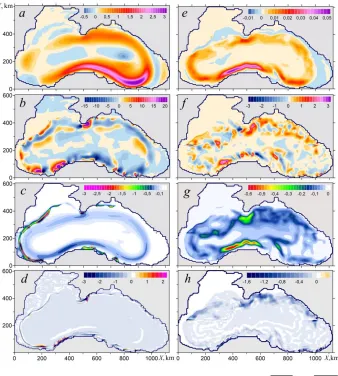
Fig. 4 shows the fields of energy transitions averaged over time. According to Fig. 4, a, the maximum of the flow of energy from the wind to the upper layer of the sea is located above the core of the average circular flow, with most of the wind energy flowing in the eastern half of the sea, and the largest values are observed to the right of the Anatolian Peninsula.

The field



K P1,



even after averaging has significant spatial heterogeneity,

especially along the core of a circular flow (Fig. 4, b). The zones in which the kinetic energy K₁ passes into the potential energy P, are located along the Caucasian coast and along the northwestern coast of Turkey. The zones with the opposite direction of energy transfer are noted to the southeast of Crimea and northwest of the Anatolian Peninsula.

F i g. 4. Spatial distribution of the time-averaged energy transitions  

1, τ

K (a),  

1,

K P (b), K D1, K2(c), K DT1, (d), K K2, 1(e), K P2, (f), K D2, (e), K DT2, (f). Unit is mJ/m

In the spatial distribution of the transition



K D₁, K₂



the characteristic feature is the presence of local areas with high values of dissipation. These areas are located on the continental slope in the form of narrow strips along the line of intersection of the interface between the layers and the bottom (Fig. 4, c), mainly in the western half of the sea along the northwestern shelf boundary and continental slope near Bulgaria and Turkey to the Bosphorus strait. In these places, the upper layer is in direct contact with the bottom. Zones of intense dissipation due to friction of the upper layer on the bottom are also noted to the south of Crimea – near Sarych Cape and the Kerch Peninsula and along the northeast coast of Turkey. In the inner sea area, where both layers exist, K1 is spent on dissipation at the liquid lower boundary of the upper layer and partially passes into K2 along the average circular flow core.

The transition of energy to dissipation due to horizontal turbulent viscosity



K DT1,



in the upper layer occurs mainly near the coastline features and along the

line of intersection of the interface between the layers and the bottom (Fig. 4, d), in the central part of the sea turbulent dissipation is small.

The lower layer obtains energy due to friction on the interface



K K2, 1



(Fig. 4, e) and due to the work of the pressure gradient force of



K P2,



(Fig. 4, f).

The transition of energy



K K2, 1



occurs in the Rim Current area, the maximum

values are noted to the northwest of Turkey. In terms of its intensity, it is significantly inferior to the transition of energy



K P2,



, which is a consequence of

baroclinic instability of the currents. The spatial distribution



K P2,



is very

uneven, which is most likely due to the bottom topography impact. The alternating maximum values of the energy flow. In the north-west of the sea, areas with positive energy transition values prevail, which corresponds to the energy transition



K P2,



into the lower layer.

Energy flow (dissipation) in the lower layer occurs due to the work of bottom friction forces and horizontal turbulent viscosity. Spatial inhomogeneities of the energy transitions



K D2,



,



K DT2,



corresponding to them (Fig. 4, g, 4, h) are

formed under the bottom topography impact and basically repeat the spatial features of the field K₂ (Fig. 3, d).

Next, the temporal variability of energy characteristics is considered. Fig. 5 shows the graphs of the time change of the energies averaged over the basin area. It can be seen that after five years of calculations, the solution goes into a quasi-equilibrium mode.

F i g. 5. Time graphs of the spatial-averaged P (a),

1

K (b),

2

K (c)

The temporal variability of the spatial-averaged energy transitions is presented in Fig. 6.

F i g. 6. Graphs of the spatial-averaged works included to the equations of energy balances K1 (a), P (b), K2 (c)

at the lower boundary of the upper layer. The graph W_G1 is predominantly located in the negative region of the ordinates, i.e., K1 becomes P, although a reverse transition is possible at some points in time. This again indicates a significant variability of energetic energy transitions (K1, P).

In the lower layer пополнение K2 is replenished mainly due to the work of the force of the pressure gradient WG 2 (Fig. 6, c).

Another source of K2 replenishment is the work of the friction force on the interface of the layers WRL 2 is very small. Energy dissipation in the lower

layer occurs due to work WRD , WAB2 .

In the quasi-equilibrium mode, the time interval in which the average characteristics of the model always remain constant regardless of the beginning of this interval, can be determined. This interval is called the statistical equilibrium period (SEP). If during the SEP the spatial-averaged energy flows will be averaged over time, then an energy diagram can be constructed for the entire sea as a whole, which shows how much energy is transmitted and in what direction, how much energy is spent on dissipation in each layer (Fig. 7). The numbers inside the rectangles correspond to the energy values in kJ/m2_{, the arrows show} the directions of transitions, and the numbers near the arrows show the average values of the energy transitions in mJ/(m2 _{s). The temporal derivatives of} the average for the SEP characteristics tend to zero.

Most of the mechanical energy of the sea (80 %) is concentrated in the available potential energy. The kinetic energy of the upper layer is 16 % and the kinetic energy of the lower layer is – 4 %. More than two thirds (69 %) of the wind energy is spent on dissipation in the upper layer due to the work of the forces of the horizontal turbulent viscosity (26 %) and the work of the friction forces at its lower boundary (43 %). Moreover, the last work can be further divided into the work of friction of the upper layer on the bottom of WRD1 at h2 = 0 (17 %) and friction on the underlying layer of WRH1, if h2 > 0 (26 %).

About 30 % of the energy coming from the wind comes to the bottom layer, only 1% of which is due to the friction force work at the interface of the layers. The main source of energy for the lower layer is the work of pressure forces, which ensures the transition of K1 into K2 through P. Energy entering the lower layer is spent on dissipation due to horizontal turbulent viscosity and bottom friction.

The figure shows that in percentage terms, the share of vortex energy is less than the energy of average currents, the ratio K₁M K₁E 2 1, PM PE 8 1,

M E 2 2 3 2

K K  . Thus, the motion in the lower layer is more vortex than in the upper one. The vortex energy makes up ~ 20% of the total mechanical energy of the system and consists of 40% of the kinetic energy and 60% of the potential energy. Most of the KE _{is concentrated in the upper layer. Despite K}E _{< K}M _in absolute value, KE _{provides most of the energy dissipation. Of the 70% of the} energy lost in the upper layer, 2/3 fall on the vortex energy dissipation.

F i g. 8. Energy diagram allowing for division of circulation into the large-scale and eddy ones

In a statistically equilibrium period, the transition K₁Mto K₁E occurs in two ways: directly and as a result of a chain of successive transitions



M M E E



1 1

K P P K . It is considered [15, 16, 17] that these energy transitions accompany the baroclinic instability of the currents, as a result of which the SEP meandering occurs and mesoscale eddies form in the upper layer.

A significant part of PE, due to the baroclinic instability of the vortices, goes into E

2

K , which is spent mainly on the vortex dissipation in the lower layer, and a small part goes into K₂M. This transition of energy can be considered as an effect of negative viscosity, when energy is transferred from smaller scales of movement to larger ones.

Besides, K₂M replenishment occurs due to PM _{as a result of the work of} the forces of the pressure gradient and as a result of the friction force work on the interface of the layers M

RL2

W . The latter work provides a direct transition



M M



1 2

K K , but its value with the parameterization used, as already noted, is

small. The vortex component W_RL2E (K₂E,K₁E) is obtained by an order of magnitude less than, and it can be neglected.

To complete the aggregate picture, the spatial energy distribution for

large-scale and eddy currents is considered below. The fields M 1

K and M 2

K

(Fig. 9, a, 9, c) generally coincide in shape with the distribution of the mean currents modulus in the upper and lower layers (Fig. 2, e, 2, g), while the areas of

maximum values M 1

K and и M 2

K are located in the southern half of the sea in the

jet stream near the Anatolian coast. Fields E E 1, 2,

K K on the contrary, are more

intense in the northern part of the sea along the continental slope. The field _PM (Fig. 9, e) practically repeats the field (Fig. 2, g), and the field _PE _{(Fig. 9, f) has} a more complex shape with two zones of maximum values, one of which is located in the north above the depths of the depth, the other – round shape – to the north of Sinop. In general, for the whole sea, it can be said that the vortex and kinetic and potential energy are mainly concentrated along the northern branch of the Rim Current. To the north-west of the Anatolian Peninsula, a maximum kinetic energy is noted in the Rim Current area.

F i g. 9. Time-averaged fields

1 M

K (a),

1 E

K (b),

2 M

K (c),

2 E

K (d), PM(e), _PE _{(f). Unit is kJ/m}2

Conclusion

The conducted energy analysis allows to draw a number of important conclusions regarding the spatial and temporal variability of the energy characteristics of large-scale circulation in the Black Sea.

the upper layer, and 30 % goes to the excitation of vortex motions in the lower layer. A small part of the kinetic energy of the vortices in the lower layer then turns into the kinetic energy of the middle currents.

The transition of the available potential energy of large-scale flows into vortex energy and further into kinetic one can serve to confirm that one of the reasons for the Rim Current meandering and the formation of mesoscale vortices is baroclinic instability.

Friction at the interface between the layers is not a significant source of movement in the lower layer of the sea and leads mainly to energy dissipation. Only ~ 2 % of the energy flow lost by the upper layer at its lower boundary increases the kinetic energy of the lower layer. Moreover, this energy transition occurs in the area of large-scale flows, the vortex friction between the layers leads to energy dissipation.

Spatial non-uniformity of wind vorticity leads to the fact that the sea receives energy from the wind, mainly in the eastern half in the Rim Current area, and loses energy in the western and north-western parts of the basin above the continental slope. The dissipation of kinetic energy occurs mainly due to friction of the upper layer about the bottom (if h2 = 0).The kinetic and potential energy of the vortices is mainly concentrated along the northern branch of the Rim Current, while in the south of the basin in Rim Current jet stream along the northwestern Anatolian coast there are maximum values of the kinetic energy of large-scale currents.

REFERENCES

1. Pavlushin, A.A., 2018. Chislennoe Modelirovanie Krupnomasshtabnoj Cirkulyacii iVihrevyh Struktur v Chernom More [Numerical Modeling of the Large-Scale Circulation andMesoscale Eddies in the Black Sea]. In: SOI, 2018. Trudy GOIN [SOI Proceedings].Moscow: SOI. Iss. 219, pp. 174-194 (in Russian).

2. Pavlushin, A.A., Shapiro, N.B. and Mikhailova, E.N., 2017. The Role of the Bottom Relief and the β-effect in the Black Sea Dynamics. Physical Oceanography, [e-journal] (6), pp. 24-35. doi:10.22449/1573-160X-2017-6-24-35

3. Holland, W.R. and Lin, L.B., 1975. On the Generation of Mesoscale Eddies and their Contribution to the Oceanic General Circulation. I. A Preliminary Numerical Experiment. Journal of Physical Oceanography, [e-journal] 5(4), pp. 642-657. doi:10.1175/1520-0485(1975)005<0642:OTGOME>2.0.CO;2

4. Holland, W.R. and Lin, L.B., 1975. On the Generation of Mesoscale Eddies and their Contribution to the Oceanic General Circulation. II. A Parameter Study. Journal of Physical Oceanography, [e-journal] 5(4), pp. 658-669. doi:10.1175/1520-0485(1975)005<0658:OTGOME>2.0.CO;2

5. Kamenkovich, V.M, Koshlyakov, M.N. and Monin, A.S., 1987. Sinopticheskie Vikhri v Okeane [Synoptic Eddies in the Ocean]. Leningrad: Gidrometeoizdat, 509 p. (in Russian). 6. Demyshev, S.G. and Dymova, O.A., 2016. Analyzing Intraannual Variations in the Energy

Characteristics of Circulation in the Black Sea. Izvestiya, Atmospheric and Oceanic Physics, [e-journal] 52(4), pp. 386-393. doi:10.1134/S0001433816040046

7. Chen, R., Thompson, A.F. and Flierl, G.R., 2016. Time-Dependent Eddy-Mean Energy Diagrams and Their Application to the Ocean. Journal of Physical Oceanography, [e-journal] 46(9), pp. 2827-2850. doi:10.1175/JPO-D-16-0012.1

8. Kang, D. and Curchitser, E.N., 2015. Energetics of Eddy–Mean Flow Interactions in the Gulf Stream Region. Journal of Physical Oceanography, [e-journal] 45(4), pp. 1103–1120. doi:10.1175/JPO-D-14-0200.1

10. Efimov, V.V. and Yurovsky, A.V., 2017. Formation of Vorticity of the Wind Speed Field in the Atmosphere over the Black Sea. Physical Oceanography, [e-journal] (6), pp. 3-11. doi:10.22449/1573-160X-2017-6-3-11

11. Efimov, V.V. and Anisimov, A.E., 2011. Climatic Parameters of Wind-Field Variability inthe Black Sea Region: Numerical Reanalysis of Regional Atmospheric Circulation. Izvestiya, Atmospheric and Oceanic Physics, [e-journal] 47(3), pp. 350-361. doi:10.1134/ S0001433811030030

12. Ivanov, V.A. and Belokopytov, V.N., 2013. Oceanography of the Black Sea. Sevastopol:

ECOSY-Gidrofizika, 210 p. Available at:

https://www.researchgate.net/publication/236853664_Ivanov_VA_Belokopytov_VN_Oceano graphy_of_the_Black_Sea_National_Academy_of_Sciences_of_Ukraine_Marine_Hydrophys ical_Institute_Sevastopol_210_p/download [Accessed: 05 June 2019].

13. Blatov, A.S., Bulgakov, N.P., Ivanov, V.A., Kosarev, A.N. and Tuzhilkin, V.S., 1984. Izmenchivost' Gidrofizicheskikh Poley Chernogo Morya [Variability of the Hydrophysical Fields of the Black Sea]. Leningrad: Gidrometeoizdat, 239 p. (in Russian).

14. Markova, N.V. and Bagaev, A.V., 2016. The Black Sea Deep Current Velocities Estimated from the Data of Argo Profiling Floats. Physical Oceanography, [e-journal] (3), pp. 23-35. doi:10.22449/1573-160X-2016-3-23-35

15. Korotaev, G.K., Oguz, T., Nikiforov, A. and Koblinsky C., 2003. Seasonal, Interannual, and Mesoscale Variability of the Black Sea Upper Layer Circulation Derived from AltimeterData. Journal of Geophysical Research: Oceans, [e-journal] 108(C4), 3122. doi:10.1029/2002JC001508

16. Zatsepin, A.G., Kremenetskiy, V.V., Stanichny, S.V. and Burdyugov, V.M., 2010. Basseynovaya Tsirkulyatsiya i Mezomasshtabnaya Dinamika Chernogo Morya pod Vetrovym Vozdeystviem [Black Sea Basin-Scale Circulation and Mesoscale Dynamics under Wind Forcing]. In: A. V. Frolov and Yu. D. Resnyanskiy, eds., 2010. Sovremennye Problemy Dinamiki Okeana i Atmosfery: Sbornik Statey, Posvyashchennyy 100-Letiyu so Dnya Rozhdeniya Prof. P. S. Lineykina [Modern Problems of Ocean and Atmosphere Dynamics. The Pavel S. Lineykin Memorial Volume]. Moscow: TRIADA LTD., pp. 347-368 (in Russian).

17. Stanev, E.V., 2005. Understanding Black Sea Dynamics: Overview of Recent Numerical Modeling. Oceanography, [e-journal] 18(2), pp. 56-75. https://doi.org/10.5670/ oceanog.2005.42

About the authors:

Andrey A. Pavlushin – Junior Research Associate, Marine Hydrophysical Institute of RAS (2 Каpitanskaya Str., Sevastopol, 299011, Russian Federation), ResearcherID: R-4908-2018, pavlushin@mhi-ras.ru

Naum B. Shapiro – leading Research Associate, Marine Hydrophysical Institute of RAS (2 Каpitanskaya Str., Sevastopol, 299011, Russian Federation), Dr.Sci. (Phys.-Math), ResearcherID: A-8585-2017, n.shapiro@mhi-ras.ru

Eleonora N. Mikhailova – Senior Research Associate, Marine Hydrophysical Institute of RAS (2 Каpitanskaya Str., Sevastopol, 299011, Russian Federation), Dr.Sci. (Phys.-Math), e.mikhailova@mhi-ras.ru

Contribution of the co-authors:

Andrey A. Pavlushin – carrying out numerical experiments, analysis of results, preparation of the paper text and graphic materials

Naum B. Shapiro – development of an energy separation algorithm for large-scale flows and eddies, analysis of the results of numerical experiments, correction of the paper, consulting support

Eleonora N. Mikhailova – validation of results, correction of the paper