TESTING FOR “RANDOMNESS” IN SPATIAL POINT PATTERNS, USING TEST STATISTICS BASED ON ONE-DIMENSIONAL INTER-EVENT DISTANCES

TESTING FOR “RANDOMNESS” IN SPATIAL POINT PATTERNS, USING

TEST STATISTICS BASED ON ONE-DIMENSIONAL

INTER-EVENT DISTANCES

M. Q. Vahidi-Asl

*

Department of Statistics, Faculty of Mathematical Sciences, Shahid Beheshti University, Tehran, Islamic Republic of Iran

Abstract

To test for “randomness” in spatial point patterns, we propose two test statistics

that are obtained by “reducing” two-dimensional point patterns to the

one-dimensional one. Also the exact and asymptotic distribution of these statistics

are drawn.

* _{E-mail: [email protected]}

1. Introduction

Data in the form of a set of points, irregularly distributed within a region of space, is usually called a

spatial point pattern. Examples, in different biological

contexts, include locations of trees in a forest, of nests in a breeding colony of birds, or of cell nuclei in a microscopic section of tissue. The locations are called

events to distinguish them from arbitrary points of the

region in question.

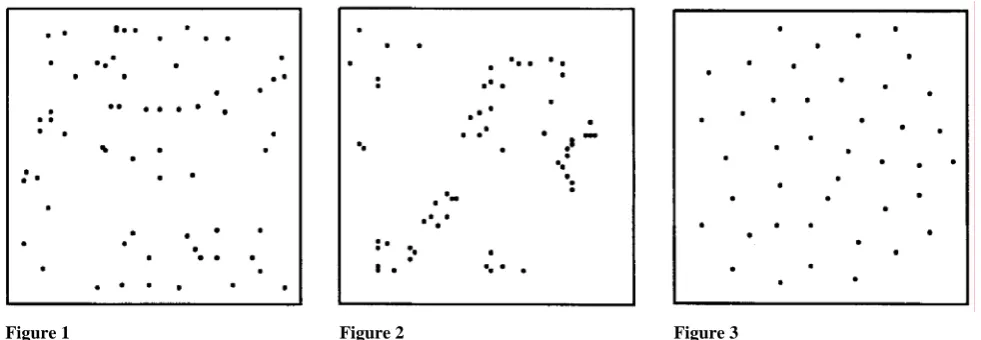
Figures 1, 2, and 3 show three spatial point patterns in a square region, all taken from Diggle [4]. The first due to Numata [5], shows 65 Japanese black pine samplings in a square of side 5.7 m, the second, extracted by [6] from [7], shows 62 redwood seedlings in a square of side approximately 23 m, and finally the third, due to Crick and Lawrence [3], shows the centers of 42 biological calls distributed more or less regularly over the unit square.

Figure 1 shows no obvious structure and might be

Keywords: Spatial patterns; Complete spatial randomness; Poisson processes

regarded as a “completely random” pattern, to be defined formally below. In Figure 2, on the other hand, the strong clustering is apparent, which is termed “aggregated” by Diggle [4] to avoid the mechanistic connotations of the perhaps more obvious term clustered. Patterns such as the ones in Figure 3 are called “regular” for obvious reasons.

The classification of patterns as regular, random or aggregated may seem an over-simplification, but it is useful at an early stage of analysis. At a later stage, this simplistic approach can be abandoned in favour of a more detailed, and essentially multidimensional description of pattern which can be obtained either by identifying different “scales of patterns” or by formulating an explicit model of the underlying process. Diggle [4] develops methods for the analysis of spatial patterns based on stochastic models, which assumes that the events are generated by some underlying random mechanism.

The hypothesis of complete spatial randomness

(henceforth CSR) for a spatial point pattern asserts that

(i) the number of events in any planar region A with

Figure 1 Figure 2 Figure 3

(ii) given n events xi in a region A, the xi is an

independent random sample from the uniform distribution on A.

Most analyses begin with a test of CSR, and there are

several good reasons for this. Firstly, a pattern for which

CSR is not rejected hardly merits any further formal

statistical analysis. Secondly, tests are used as a means of exploring a set data, rather than because rejection of

CSR is of intrinsic interest. Greig-Smith, in the

discussion of Bartlett [2], has emphasized that ecologists often know CSR to be untenable but

nevertheless use tests of CSR as an aid to the

formulation of ecologically interesting hypotheses concerning pattern and genesis. Thirdly, CSR acts as a

dividing hypothesis to distinguish between patterns which are broadly classifiable as “regular” or “aggregated”.

There are numerous methods for testing a point pattern against CSR on top of which is the use of Monte

Carlo tests [1].

Quite generally, let u1 be the observed value of a statistic U and let ui, i=2,…, s, be the corresponding

values generated by independent random sampling from the distribution of U under a simple hypothesis H. Let

u(j) denote the jth largest amongst ui, i=1,…, s. Then,

under H,

{

u₁ u_{( )}

}

s 1, j 1, ,s,

P = _j = − = K

and rejection of H on the basis that u1 ranks kth larger or higher gives an exact, one-sided test of size k/s. Usually, s is taken as 100 in most examples. For complete details

and other related topics, we refer the reader to Ref. [4]. A complete and updated list of statistical tests for testing CSR, with less emphasis on Monte Carlo tests, is

given in chapter 8 of the more recent book by Cressie [8].

Our concern here is to introduce test statistics whose

exact and asymptotic distributions are known and test

CSR against data without using any simulation.

Therefore it may be included among the many simple existing tests, nevertheless it proves to be as effective as Monte Carlo tests, as emphasized in [4]. In Section 2 we introduce these statistics and some theoretical results regarding their distribution, and in Section 3 we use this method on the data given in Figures 1-3 [4].

2. Theoretical Results

Since the statistics to be introduced are based on points distributed along a line with exponential distribution for the distance between two consecutive points, therefore we consider the one-dimensional case first.

Let the points X1,…, Xn+1 be distributed randomly along some stretch of a line so that the random variables

n i

X X

T_i= _i+1− _i, =1,2,_K,

are iid. The random process

{ }

Tn _n≥1 with Tn=Xn–Xn–1,

n=1,2,…, forms an iid sequence of random variables

with mean λ–1 _{if and only if}

{ }

_{is a labeling of a} homogenous Poisson process of intensity λ [9]. Here, the points

1 ≥

n n

X

{ }

Xi _1≤i≤n+1 are a restriction of a Poisson point

process to some stretch of a line. Let c be a constant.

We place line segments of length c on every point Xi

along the supporting line of the Xi’s so that Xi is the

midpoint of this line segment. These lines either overlap or there is a “gap” between two consecutive line segments. If we denote the gap between Xi and Xi+1 by

Yi, then we have

(

T c

)

, i 1,2, ,n,

Yi= i− = K

+

in which x+=max(x,0). This holds because the right half

of this point and the left half of the line of length c

centering at Xi+1 extends to the left of this point, and there is no “gap” between Xi and Xi+1 if and only if

, and therefore Y

c

T_i≤ i=0.

Let . We discuss the distribution of U

first.

∑

=

= n

i Yi

U ₁

Theorem 1. If the T1, T2,…, Tn are iid random variables

with a common exponential distribution with mean λ–1 then

(

)

(

)

(

e

)

( )

u

e u jc h j n u F n c n j j n c j U 0 1 1 1 ) ( δ λ λ − = − − − + − + ⎟ ⎠ ⎞ ⎜ ⎝ ⎛ =

∑

where

(

)

, , ) ( , 2 , , , , ) ( 1 1 1 1 c z e e z h j dt e t z h c T c T z T P z h z t z c t j j i i i j ≥ − = ≥ − = ⎟⎟ ⎠ ⎞ ⎜⎜ ⎝ ⎛ ≥ ≥ ≤ = − − − − =

∫

∑

λ λ λ λ K and ⎩ ⎨ ⎧ ≥ < = t x t x x t if 1 if 0 ) ( δ .

Proof. Let N be the number of Ti, s such that ,

then,

c Ti≥

(

)

(

)

(

)

(

)

(

, ,

)

( ) , , ) ( 0 1 1 1 0 1 1 u c T c T P j N u c T P j N u c T P u c T P u U P u F n n j n i i n j n i i n i i U δ < < + ⎟ ⎠ ⎞ ⎜ ⎝ ⎛ _{− ≤ =} = ⎟ ⎠ ⎞ ⎜ ⎝ ⎛ _{− ≤ =} = ⎟ ⎠ ⎞ ⎜ ⎝ ⎛ ≤ − = ≤ =

∑ ∑

∑ ∑

∑

= = + = = + = + K

Now by using the iid property of Ti, s we have

(

)

} (

1

)

( )

, , , , , ) ( 0 1

1 1 1

u e c T c T c T c T u c T P j n u F n c n j n j n i j i U δ λ − + = = + − + < < ⎩ ⎨ ⎧ _{− ≤ ≥ ≥} ⎟ ⎟ ⎠ ⎞ ⎜ ⎜ ⎝ ⎛ =

∑

∑

K K

(

)

} (

)

{

} (

)

(

)

(

)

(

)

(

)

(

)

∑

∑

∑

∑

∑

∑

∑

= − − − − − − = = − + = = − + = = − + − + ⎟ ⎟ ⎠ ⎞ ⎜ ⎜ ⎝ ⎛ = − + − × × ⎭ ⎬ ⎫ ⎩ ⎨ ⎧ ≥ ≥ + ≤ ⎟ ⎟ ⎠ ⎞ ⎜ ⎜ ⎝ ⎛ = − + < < × × ⎭ ⎬ ⎫ ⎩ ⎨ ⎧ ≥ ≥ + ≤ ⎟ ⎟ ⎠ ⎞ ⎜ ⎜ ⎝ ⎛ = − + < < ⎩ ⎨ ⎧ _{− ≤ ≥ ≥} ⎟ ⎟ ⎠ ⎞ ⎜ ⎜ ⎝ ⎛ = n j n c j n c j n c j n c n j j i j i n c n j n j j i j i n c n j n j n i j i u e e u jc h j n u e e c T c T u jc T P j n u e c T c T P c T c T u jc T P j n u e c T c T c T c T u c T P j n 1 0 0

1 1 1

0 1

1 1 1

0 1

1 1 1

) ( 1 1 ) ( 1 1 , , ) ( 1 , , , , ) ( 1 , , , , , , , δ δ δ δ λ λ λ λ λ λ K K K K K K K

in which as

mentioned in the statement of the theorem. But

) , , , ( )

( =

∑

j₌₁ ≤ ₁≥ ≥

i i j

j z P T zT c T c

h _K

∫

∫ ∑

∫

∑

≥ − = ⎟⎟ ⎠ ⎞ ⎜⎜ ⎝ ⎛ ≥ ≥ − ≤ = ⎟⎟ ⎠ ⎞ ⎜⎜ ⎝ ⎛ = ≥ ≥ ≤ = − − − − = − ∞ = z c t j z c t j i j i T j i j j i j j dt e t z h dt e c T c T t z T P dt t f t T c T c T z T P z h . 2 , ) ( , , , ) ( | , , , ) ( 1 1

1 1 1

0 1 1 λ λ λ λ K K

The statement for h1(z) is obvious. □

The application of this result for computing probabilities needed in the last section requires tedious recursive integrations. An upper bound for the probability P(U≤u) may be obtained as in the

following corollary.

Corollary 1. With Ti’s as in Theorem 1, we have

{

( ),

}

, min ) ( ) ( 0

∑

= ⎟ ⎟ ⎠ ⎞ ⎜ ⎜ ⎝ ⎛ ≤ = ≤ n j j j U b u a j n u F u U P where, ⎭ ⎬ ⎫ ⎩ ⎨ ⎧ _{≤ +} =

∑

= − j i i cj

j u e P T jc u

a

1

)

( λ

and

(

1 c

)

n j. jc

j e e

Proof. Let u > 0. Then

(

)

} , , , , , { }. , , , , , { ) ( ) ( 1

0 1 1

1

0 1 1

c T c T c T c T u jc T P j n c T c T c T c T u c T P j n u U P u F n j n j n i j i n j n j n i j i U < < ≥ ≥ + ≤ ⎟ ⎟ ⎠ ⎞ ⎜ ⎜ ⎝ ⎛ = < < ≥ ≥ ≤ − ⎟ ⎟ ⎠ ⎞ ⎜ ⎜ ⎝ ⎛ = ≤ = + = = + = = +

∑

∑

∑

∑

K K K K But,

(

_c

)

n j j i i n j j i i n j j i j i j e u jc T P c T c T u jc T P c T c T c T c T u jc T P u c − − = + = + = − ⎟⎟ ⎠ ⎞ ⎜⎜ ⎝ ⎛ + ≤ = ⎟⎟ ⎠ ⎞ ⎜⎜ ⎝ ⎛ < < + ≤ ≤ ⎟⎟ ⎠ ⎞ ⎜⎜ ⎝ ⎛ < < ≥ ≥ + ≤ =

∑

∑

∑

λ 1 , , , , , , , , ) ( 1 1 1 1 1 1 K K K and . ) 1 ( , , , , , ( )

( _{1 1}

j n c jc n j j j e e c T c T c T c T P u c − − − + − = < < ≥ ≥ ≤ λ K K

Therefore cj(u)≤min{aj(u),bj} and the result follows.

Note that aj(u) may be computed using χ2 tables. □

The above result gives approximate values of the probabilities needed later on in the next section, but as is seen, it still requires lengthy calculations, which we are trying to avoid. It is fortunate that the asymptotic distribution for U is very easy to come by and at the

same time, as will be shown, very helpful.

Theorem 2. Let T1,…, Tn be iid random variables with a

common exponential distribution with mean λ–1_{. Then} the random variable has an asymptotic normal distribution with mean and variance

.

+ =

∑

−

= n₁( )

i Ti c

U

c

e nλ−1 −λ

) 2 (

2_e c _e c

nλ− −λ − −λ

Proof. Considering the iid sequence {Tn} we note that

the sequence {(Tn-c)+} is iid also, therefore we can

apply the central limit theorem, iid case, to the latter sequence and conclude that

σ μ n n c T U n

i i− −

=

′

∑

=1( )+

has an asymptotic standard normal distribution, once we show that

c

e c T

E λ λ

μ_{= −} +₌ −1 −

1 ) ( and . ) 2 ( ) var( 2 1 2 ∞ < − = − = − − − + c c _e e c T λ λ λ σ But , ) ( ) ( 1 0 ) ( 1 c c u c t e du ue dt e c t c T E λ λ λ λ λ − − ∞ _{− +} ∞ ₋ + = = − = −

∫

∫

and , 2 ) ( ] ) [( 2 0 2 2 2 1 c y c c t e dy e y e dt e c t c T E λ λ λ λ λ λ − − ∞ ₋ − − ∞ ₋ + = = − = −

∫

∫

hence the desired result. □

For arbitrary n, we may use a statistic W whose

definition and distribution, both exact and asymptotic, are very easy to find.

Theorem 3. Let W =

∑

n_i=11{T_i>c} where Ti, s are as in

Theorem 2 and 1A is the indicator function of the set A.

Then W has a binomial distribution with a success

probability of c. □

e p= −λ

The above results are readily applicable to “line data” or points randomly distributed along a line. The idea of exploiting the statistic U above is very simple: if the n+1 points are “almost regularly” distributed along their

supporting line, and c is chosen close to the average

distance between all of the points, then U will be

“small”. For points randomly distributed under CSR

assumption, the value of U should be “moderate” and

for “aggregated data” or points showing somehow clustering, the value of U should be “large”. We now try

to adapt it to planar data. In the next section, we will use the above statistics to test the data referred to in the Introduction.

Consider a rectangle A with sides a and b. The

hypothesis of CSR is valid in this rectangular region.

We divide the sides with length a and b to l and m

rectangles with sides a and

m

b _{and rectangles with sides}

b and

l

a_{. Now consider the “horizontal” rectangles first.}

If we show these rectangles by A1, A2,…, Am, we project

all the points inside Aj; j=1,2,…,m on the “base” of the

rectangle, i.e., the side with length a. If we denote two

consecutive projections in the rectangle Aj by Xij and

Xi+1,j and the distance between the points Xij and Xi+1,j by

Tij, then under CSR

t m b ij t e

T

P( > )= −λ

and therefore Tij has an exponential distribution with

mean m(λb)-1, and hence we are back to the

one-dimensional case again. Doing the same on all the strips

A1,…, Am, we may consider the statistic

∑

₋ +

=

j i

ij c

T U

,

) (

which is the sum of n-m independent identically

distributed random variables with a common exponential distribution with mean m(λb)-1. Using the

same procedure for vertical strips, we obtain a statistic

∑

_{′− ′}+

=

j i

ij c

T V

,

) (

which is the sum of n-1 independent identically

distributed random variables with a common exponential distribution with mean l(λa)-1. Let c=_nma_−m and _{c n}lb_l

− =

′ . As for the “linear” data, “small values” of

U and V simultaneously correspond to the “regular” data

and “large values” of U and V correspond to

“aggregated” data. Therefore, we will reject the CSR

hypothesis whenever

). (

)

(U≤u₁ and V≤v₁ or U≥u₂ and V≥v₂

3. Application to Certain Data

We now apply the statistics presented in Theorems 2 and 3 to the data given in Figures 1-3 of the Introduction, but before doing so we note that these three sets of data are distributed in a square region, so we may take m=l and c=c′ in which case U and V

have the same distribution and therefore we may reject the CSR hypothesis whenever

) , max( )

,

min(u1v1 or U u1v1

U≤ ≥ .

We consider the three cases separately.

3.1. Location of Japanese Black Pine Trees

Consider the data presented in Figure 1 of the

Introduction. We take m=n=5. We have doubled the size

of squares in Figures 1-3 so that we have a square with 10 cm sides in this case. Therefore, according to Theorem 2,

) 2 ( )

2 ( , ) 2

( 1 2 1 2 c 2 c

U c

U n λ e λ σ λ ne λ e λ

μ ₌ − − ₌ − − ₋ − _.

To obtain numerical values of μU and σU we need an

estimate for λ. Under CSR, λˆ= 65_A =0.65 is the

maximum likelihood estimate of λ [4].

Also in order to take into account the “gaps” between the two events which are the “last” and “first” events in two consecutive rectangular strips, we take n=65. This

is tantamount to “piecing together” all the strips and obtaining one strip of 5×10 cm long and 2 cm wide. This is reasonable under the CSR hypothesis as long as

we ignore the edge effects. We will do the same in Sections 3.2 and 3.3 without further mentioning. Therefore,

. 8 . 16 ,

9 . 11

81 . 4 ,

45 . 18

1

1= =

≈ ≈

v u

U

U σ

μ

We have

0869 . 0 ) 9 . 11 ( < =

=PU

p .

Note that we have a two-sided test here, that the attained significant level will be 2×(0.0869)=0.1738, and hence the CSR hypothesis is accepted.

It should be noted that doubling the one-sided

P-values in asymmetric cases is somewhat controversial

but is advocated by some authors, including R. A. Fisher [10]. We will adhere to this fact without further mentioning.

We now apply Theorem 3 for this set of data. The statistic has a binomial distribution with

success probability . Here . Since

n is large enough, we may use the normal

approximation to the binomial. This time “small values” of W correspond to “aggregated” data and “large

values” of W correspond to “regular” ones. The

observed value of W here is w

∑

= >

= n

i T_i c

W ₁1_{{ }}

c

e

p= −λ p=e−1≈0.37

1=20 for the horizontal strips and w2=23 for the vertical strips. Hence,

1539 . 0 ) 02 . 1 ( ) 20 ( ) , min(

(W< w₁ w₂ =PW< ≈P Z<− = P

Therefore the attained significant level is 2(0.1530)= 0.3078 and the CSR hypothesis is accepted again.

3 . 28 ) , max( , 26 ,

3 . 28 ,

92 . 4

, 45 . 18 ,

80 . 0 62 50 ,

100 62 ˆ , 62

2 1 2

1= = =

=

= ≈

= =

=

u u u

u c n

U

V

σ

μ λ

Therefore,

0228 . 0 ) 00 . 2 ( ) 92 . 4

45 . 18 3 . 28 ( ) 3 . 28

(U> ≈P Z> − =P Z> = P

Hence the attained significant level is 0.0456 and the

CSR hypothesis is rejected.

Now applying Theorem 3 and noting that w1=14 for the horizontal strips and w1=11 for the vertical strips, we have μW=22.88, σW=3.80, and therefore

001 . 0 ) 12 . 3 ( ) 11

(W≤ ≈P Z≤− <

P ,

and the CSR hypothesis is emphatically rejected.

3.3. Locations of 42 Cell Centers

For this set of data, we have u1=9.3 for the horizontal strips and u2=7.5 for the vertical ones, μU=18.45,

σU=5.99. Hence

0336 . 0 ) 83 . 1 ( ) 5 . 7

(U< ≈P Z<− =

P .

The attained significance level is 2(0.0336)=0.0676, and we may be inclined to reject the CSR hypothesis.

Regarding the other statistic presented in Theorem 3, we have μW=15.59 and σW=3.128. Since w1=13 for the horizontal strips and w2=18 for the vertical ones, therefore

209 . 0 ) 812 . 0 ( ) 13

(W< ≈P Z<− =

P ,

and this leads to the acceptance of the CSR hypothesis,

contrary to what we except as a result of applying the majority of the tests presented by [4].

To investigate the effects of increasing the number of the rectangular strips partitioning the region A, we take m=l=10. Once again μW=15.54, σW=3.128, w1=10 and

w2=14. Hence

384 . 0 ) 77 . 1 ( ) 10

(W< ≈P Z<− =

P ,

and this time the CSR hypothesis is rejected.

It is interesting to use Theorem 2 again for the new partitioning. This time, μU≈36.76, σU≈11.95, u1=26.2,

u2=18.1, and

0594 . 0 ) 56 . 1 ( ) 1 . 18

(U< ≈P Z<− ≈

P ,

so the result hints to the acceptance of the CSR

hypothesis. Even partitioning the region to m=l=15

strips does not lead to the rejection of CSR hypothesis

for this set of data. This may be an indication of the weakness of these tests against ”regular” alternatives.

But referring to the statistical tests discussed in [4], we note that some of these tests justify the acceptance of this set of data as being completely spatial random. The majority of the tests supporting the “regularity” hypothesis are specifically based on “small distances”. Examining the empirical distribution function plot, a complete absence of small inter-event distances is observed [4]. Translating this idea in terms of the statistic, denoted by W in Theorem 2 of Section 3.2, we

may consider a variant of this statistic, defined by

∑

≤′

= ′ n

j i

c Tij W

, { }

1

where c´ is any positive constant. Though there is an

element of arbitrariness in choosing the value of c´, we

may note that any reasonable “extreme value” would suffice for this purpose. For our examples, we choose

2

c

c′= where

n ma

c= when m=l. W´ denotes the number

of inter-event distances shorter than c´, and has a

binomial distribution with parameters n and

where (λ´)

c

e p=1− −λ′′ -1 _{is the mean of}

Tij. For the pattern given as

the location of 42 cell centers in Figure 3, we have 60

. 0

≈

c , w₁′=7, w₂′=6, therefore the attained significance level is approximately

) 60 . 3 ( 2 ) ) 61 . 0 )( 39 . 0 ( 42

39 . 42 5 (

2P Z< − = P Z<−

and the CSR hypothesis is emphatically rejected.

For the location of Japanese black pine trees given in Figure 2, we have c′≈0.34, , , so the

attained significance level is approximately

24

1′=

w w₂′=19

) 601 . 1 ( 2P Z<−

which leads to the acceptance of the CSR hypothesis.

Finally for the locations of 62 redwood seedlings presented in Figure 2, we have c′≈0.40, w₁′=38,

42

2′=

w , and hence the attained significance level is approximately,

) 64 . 4 ( 2P Z>

which leads to the emphatic rejection of the CSR

hypothesis.

Remark. We should note that even though we have

additional events, the number of which is proportional to the area of the added area. This is justified under the

CSR hypothesis.

Another advantage of this method is that, we may allow the existence of some “excluded” areas in the study region, such as lakes in a breeding colony of birds or deserts in a country in studying population centers.

Acknowledgements

The helpful comments of the referees are gratefully acknowledged.

References

1. Barnard, J. A. Contribution to the discussion of Prof. Bartlett paper. J. R. Statis. Soc., B25, 294, (1963).

2. Bartlett, M. S. Two-dimensional nearest neighbour systems and their ecological applications. In: Statistical Ecology, Patil, G. P., Pielou, E. C. and Waters, W. E. (Eds.), University Park, Pennsylvania State University

Press, pp. 179-194, (1971).

3. Crick, F. H. C. and Lawrence, P. A. Compartments and polychones in insect development. Science, 189, 340-347, (1975).

4. Diggle, P. J. Statistical analysis of spatial point patterns. Academic Press, London, (1983).

5. Numata, M. Forest vegetation in the vicinity of Choshi. Coastal flora and vegetation at Choshi, Chiba Prefecture IV. Bull. Choshi Marine Lab. Chiba Univ., 3, 28-48 [in Japanese], (1961).

6. Ripley, B. D. Modelling spatial patterns (with discussion). J. R. Statist. Soc., B39, 172-212, (1977). 7. Strauss, D. J. A model for clustering. Biometrika, 62,

467-475, (1975).

8. Cressie, N. A. C. Statistics for spatial data. John Wiley & Sons Inc., New York, (1993).

9. Cox, D. R. and Isham, V. Point Processes. Chapman & Hall, London, (1980).