Fitting Second-order Models to Mixed Two-level and Four-level Factorial Designs: Is There an Easier Procedure?

Please cite this article as: W. A. A. Alqaraghuli, A. F. M. Alkarkhi, H. C. Low, Fitting Second-order Models to Mixed Two-level and Four-level Factorial Designs: Is There an Easier Procedure?, International Journal of Engineering (IJE), TRANSACTIONS B: Applications Vol. 28, No. 11, (November 2015) 1644-1650

International Journal of Engineering

J o u r n a l H o m e p a g e : w w w . i j e . i r

Fitting Second-order Models to Mixed Two-level and Four-level Factorial Designs:

Is There an Easier Procedure?

W. A. A. Alqaraghulia_{, A. F. M. Alkarkhi}b_{* , H. C. Low} a

a_{School of Mathematical Sciences, Universiti Sains Malaysia, Penang, Malaysia} b_{School of Industrial Technology, Universiti Sains Malaysia, Penang, Malaysia}

P A P E R I N F O

Paper history: Received 29 June 2015

Received in revised form 04 October 2015 Accepted 16 October 2015

Keywords:

Two-level Factorial Design Four-level Factorial Design Response Surface Methodology

A B S T R A C T

Fitting response surface models is usually carried out using statistical packages to solve complicated equations in order to produce the estimates of the model coefficients. This paper proposes a new procedure for fitting response surface models to mixed two-level and four-level factorial designs. New and easier formulae are suggested to calculate the linear, quadratic and the interaction coefficients for mixed two-level and four-level factorial designs regardless of the number of factors included in the experiment. The results of the proposed procedure are in agreement with the results of least squares method. This paper could motivate researchers to study the possibility of applying a fixed formula to all factorial designs.

doi: 10.5829/idosi.ije.2015.28.11b.12

1. INTRODUCTION1

The concept of factorial designs was first introduced by Fisher in the mid- 1920’s [1]. Researchers furthered the development of factorial design by introducing new methods, designs or applications. The concept of factorial designs became clear in the 1937 when Yates introduced a new method for analyzing two-level designs [2, 3]. Davies applied the idea of two-level designs to three-level designs, fitting response surface models to the latter [2]. Interest in factorial designs and their contribution to various fields increased in the 1960’s. Margolin [4] combined Yates’ two-level designs and Davies’ three-level designs to develop mixed factorial designs, a procedure for analyzing and fitting response surface to mixed designs. Draper and Stoneman [5] studied the number of experiments (runs) required to fit response surface models to mixed level and three-level factorial designs and mixed two-level and four-two-level designs. Factorial designs increasingly contributed to experiment design and

1_{*Corresponding Author’s Email: [email protected] (A. F. M.} Alkarkhi)

analysis and became the focus of many researchers, thereby necessitating a review of its impact. Herzberg and Cox [6] reviewed roughly 800 works that had been published since 1957 and provided a detailed bibliography for researchers. Addelman [1] reviewed factorial design application in works published from 1965 to 1972 and found that most of the studies utilized fractional factorial designs. Edmondson [7] fit a second-order model to a four-level design using pseudo-factors to represent the four-levels. Bisgaard [8] presented a method for accommodating four-level factors in two-level designs. This method converts two or more columns to accommodate multi-level factors. Abbas et al. [9] proposed new formulae for analyzing two-level designs and fitting a first-order response surface model to this type of experiment. Abbas [10] also fit a second-order model to three-level designs. Abbas and Low [11] presented a new procedure for analyzing mixed two-level and three-two-level designs. Wasin et al. [12] fit response surface to a four-level design using the coefficients of an orthogonal polynomial.

special knowledge to carry out statistical analysis, creating an additional challenge to the researchers.

Design and analysis of experiments have been widely used by researchers from different fields for instance, different engineering areas, environmental technology, food science and other disciplines to carry out different experiments such as four-level design which was used by kovo [13] and response surface methodology which was used by Hosseinpour et al. [14], Sayyar Kavardi et al. [15] and Yahyaei et al. [16] for optimization different experiments.

The objectives of this research are 1) to investigate the possibility of using the linear coefficients of a polynomial contrast for fitting response surface models to mixed two-level and four-level factorial designs, thereby avoiding use of the least squares method, which is especially cumbersome when the number of independent variables is greater than two, and 2) to investigate the possibility of calculating each coefficient of the model individually. This procedure will streamline the method for fitting response surface models to mixed two-level and four-level factorial designs.

2. MIXED TWO-LEVEL AND FOUR-LEVEL FACTORIAL DESIGNS

The two-level and four-level factorial experiment is a factorial design with mixed levels, p factors each at two levels and q factors each at four levels and is denoted

by 2p4q. The simplest design for two-level and four-level factorial design has two factors, one at two four-levels and one at four levels. The total number of runs required for 1 1

4

2 is 8 runs for one replicate [2, 17].

3. PROPOSED PROCEDURE

The proposed procedure for fitting response surface models to a 2p4q experiment splits the process into two experiments, type 2p and type 4q, then analyzes each experiment separately to find the linear, quadratic and interaction coefficients between the factors with equivalent levels.

The proposed procedure for fitting a response surface model to a mixed two-level and four-level factorial design is based on combining the two procedures for fitting experiments of type 2 [9] and p for experiments of type 4 [12]. The data should be q normally distributed.

The formulae for fitting two-level factorial design based on two factors [9] are:

n X for Contrast

b_l l

4

 l1, 2, ..., p, for linear

coefficients and the interaction:

n

q X l X for Contrast b_lq

4

 lq

and the formulae for four-level factorial design [4] are: a. Linear coefficient

n X for contrast Linear

b_L L

 

20

q L1, 2, ...,

b. Quadratic coefficient

n X for contrast Quadratic

bLL  _ L

16

c. Interaction coefficient

n X X for contrast Linear

bLQ  _ L Q 400

, LQ

Below are the formulae for intercept and interaction between factors that have two levels and factors that have four levels will be derived in the next section.

4. PROPOSED FORMULAE FOR INTERCEPT AND INTERACTION

Consider a second-order response surface model with p factors each at two levels (X1, X2, …, Xp) and

q

factors each at four levels (Z1, Z2, …, Zq) as given below:

i qi pi pq i i qi i q q q

i i qi qq i qi q

i i pi i p p p

i i pi p i i i

Z X Z

X Z Z

Z Z Z Z

Z

Z Z X X b

X X b X b X b X b b Y

 

 

  



 

 

 



 

   

   



     

... ... ...

... ...

...

1 1 11 ) 1 ( ) 1 (

2 1 12 2 2

1 11

2 2 1 1 ) 1 ( ) 1 (

2 1 12 2

2 1 1 0

k i1, 2, ...,

(1)

The levels of each factor represent the coded form, which is similar to the linear coefficients of the orthogonal contrast. The relationship between actual and coded variables for two levels is:

2 / ) (

2 / ) (

Low Highe

Low High C X

   

and for four levels is:

2 / levels) e consecutiv two

any of Range (

4 / ) (

levels all of

Average a1 a2 a3 a4

C

X    

The model in Equation (1) obeys some constraints. The constraints are obtained from the linear coefficients of the orthogonal polynomial contrast for four levels (-3 -1 1 3) and the contrast for two levels (-1 1). The constraints are as follows:

a. Constraints for the factors at two levels:

1- _

 

k

i i X

1

0 2-





k

j i

3- _   k j i j i X

X2 0 4- 

  k j i j iX X 2 0

5- _{ 0}   k h j i h j iX X

X 6-    k i i k X 1 2 7-_   k j i i j

k X X )2 (

b. Constrains for the factors at four levels:

1- 0 1    k i i

Z 2-

  k j i j iZ

Z 0 3-    k i i iZ Z 1 2 0 4-_   k j i i j

Z

Z 2 0 5-

1 1

2 _{20 4}

  

k q

i i Z 6- 1 1 4 4 164    

k q

i i Z 7-     k j i q j iZ

Z2 2 2

4 400 8- 0     k z j i i j z

Z Z Z 9-     k j i q j iZ

Z )2 400 4 2

(

c. Constraints for the joint effects between factors at two levels and factors at four levels:

1- _

   _   k i p q i X i Z 1 1 1 2 ) 2 4 ( 40 ) (

2- ₀

1 2

1 1

2 _{ }

       k i i i k i k i i iZ XZ X

i Z i X

3- _{ }

      k l j i k l j i l j iZ X Z l Z j X i X 0

The formula for the intercept bo for mixed two-level and four-level factorial design can be derived by summing Equation (1) over i and applying the constraints that yield the formula in Equation (2).

q qqZ b Z b Z b Y

b0  11 1 22 2... (2)

where

k Z Z_i i

2

, and k is the total number of

observations.

The formula for the interaction coefficient between factors at two levels and four levels can be derived by multiplying Equation (1) by Xli ZLi and summing over i, which give the formula in Equation (3).

∑ ∑ 2

) ( li Li lL

i Li

liZ Y X Z X 

(3)    2 ) ( _{li Li}

i Li li lL Z X Y Z X

 l1, 2, ...,p, L1, 2, ...,q

The formula for the interaction coefficient between factors at two levels and four levels in Equation (3) can be written in terms of linear joint contrast. To illustrate the procedure, consider a 2242 experiment without losing information from the general formula.

TABLE 1. A design with four factors where X1 and X2 have

two levels each, and Z1 and Z2 have four levels each

Z1 Z2

X1 -1 -1 1 1

X2 -1 1 -1 1

-3 -3 Y1 Y17 Y33 Y49

-1 -3 Y2 Y18 Y34 Y50

1 -3 Y3 Y19 Y35 Y51

3 -3 Y4 Y20 Y36 Y52

-3 -1 Y5 Y21 Y37 Y53

-1 -1 Y6 Y22 Y38 Y54

1 -1 Y7 Y23 Y39 Y55

3 -1 Y8 Y24 Y40 Y56

-3 1 Y9 Y25 Y41 Y57

-1 1 Y10 Y26 Y42 Y58

1 1 Y11 Y27 Y43 Y59

3 1 Y12 Y28 Y44 Y60

-3 3 Y13 Y29 Y45 Y61

-1 3 Y14 Y30 Y46 Y62

1 3 Y15 Y31 Y47 Y63

3 3 Y16 Y32 Y48 Y64

Suppose there are four factors: X1, X2 at two levels and Z1, Z2 at four levels. The design for this experiment is given in Table 1. Consider the formula for ₁₁,

   ₂ 1 1 1 1 11 )

( _{i i}

i i i Z X Y Z X  ₍₄₎

The denominator of Equation (4) equals to:

320 ) 2 4 ( 40 ) 2 4 ( 40 )

( 1 1 2 1 1  11 

 q p

i iZ

X . This is equal to

8

40 , where 8 represents the number of replicates at each joint level. The numerator of Equation (4) is:

) ( 3 ) ( ) ( ) ( 3 61 45 57 41 53 37 49 33 32 16 28 12 24 8 20 4 62 46 58 42 54 38 50 34 31 15 27 11 23 7 19 3 63 47 59 43 55 39 51 35 30 14 26 10 22 6 18 2 64 48 60 44 56 40 52 36 29 13 25 9 21 5 17 1 64 1 1 1 Y Y Y Y Y Y Y Y Y Y Y Y Y Y Y Y Y Y Y Y Y Y Y Y Y Y Y Y Y Y Y Y Y Y Y Y Y Y Y Y Y Y Y Y Y Y Y Y Y Y Y Y Y Y Y Y Y Y Y Y Y Y Y Y Y Z X i i i i                                                                   (5)

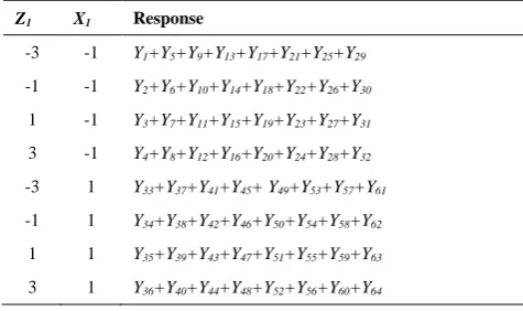
Table 2 for X1 and Z1, are summed in the cells. Similar tables can be constructed for X1Z2, X2Z1, and X2Z2. From Table 2, the linear joint contrast for X₁Z₁ is:

] )[ 1 )( 3 ( ... ] )[ 1 )( 1 ( ] )[ 1 )( 3 (

64 60 56 52 48 44 40

36 30

26 22 18

14 10 6 2 29

25

21 17 13 9 5 1

Y Y Y Y Y Y Y

Y Y

Y Y Y

Y Y Y Y Y

Y

Y Y Y Y Y Y

      

     

   

 

     

(6)

TABLE 2. The results for factors X1 (at two levels) and Z1 (at

four levels)

Z1 X1 Response

-3 -1 Y1+Y5+Y9+Y13+Y17+Y21+Y25+Y29

-1 -1 Y2+Y6+Y10+Y14+Y18+Y22+Y26+Y30

1 -1 Y3+Y7+Y11+Y15+Y19+Y23+Y27+Y31

3 -1 Y4+Y8+Y12+Y16+Y20+Y24+Y28+Y32

-3 1 Y33+Y37+Y41+Y45+ Y49+Y53+Y57+Y61

-1 1 Y34+Y38+Y42+Y46+Y50+Y54+Y58+Y62

1 1 Y35+Y39+Y43+Y47+Y51+Y55+Y59+Y63

3 1 Y36+Y40+Y44+Y48+Y52+Y56+Y60+Y64

TABLE 3. The actual and coded form for the selected

variables

Factor level X1 coded X2 Coded X3 coded

a1 5 -1 3 -3 15 -3

a2 9 1 4 -1 20 -1

a3 6 1 25 1

a4 8 3 30 3

The result in Equation (6) is the same as the result in Equation (5); therefore, the numerator of Equation (4) can be written as the linear joint contrast for X₁ and

1

Z . Thus, Equation (4) can be written using linear contrast as given below:

8 40 )

(

1 1 2

1 1

1 1

11  _



 Linear contrast for XZ

Z X

Y Z X

i i

i i i



where 8 represents the number of replicates at the joint levels. Similarly, the same steps can be used to find the formula for other coefficients. In general, let n represent the number of replicates at the joint levels, then the formula becomes:

n Z X for contrast

Linear _L

lL

l

 

40

 (7)

In summary, it can be said that the proposed procedure will eliminate the need to use the least squares method,

which is particularly cumbersome when the number of independent variables is more than two, making it difficult to find the inverse matrix. Furthermore, the proposed procedure provides a simple way to check individual coefficients without affecting other coefficients in the model. Alternatively, the least squares method results in a different intercept for each variable and possibly different coefficients when all terms are included in the model.

5. A NUMERICAL EXAMPLE

The following example illustrates the steps of the proposed procedure and compares the results with the least squares method. The calculations for the new procedure were done by using normal calculator to show that the new procedure is simple whilst SPSS version 20 was used for the least squares method. The production of lactic acid from mango peels using the bio-fermentation method was investigated. The effect of three factors on lactic acid yield was studied: initial medium pH (X1) at two levels (5 and 9), fermentation time (X2) at four levels (2, 4, 6 and 8 days) and temperature (X3) at four levels (15, 20, 25, and 30°C). The design used to run this experiment is a 2142 type. The total number of runs is 64-run with two replicates. The levels of each factor in actual and coded form are given in Table 3. The researcher wants to fit a second-order response surface model to this experiment. The model is given in Equation (6).

2 1 23 2 1 12 1 1 11 2 2 22

2 1 11 2 2 1 1 1 1 0

Z Z Z X Z X Z

Z Z Z X b b Y

 

 

  

 

 

    

(6)

Both the least squares method and the proposed procedure will be used to fit the model in Equation (6). Fitting a response surface model to this type of experiment using the proposed procedure requires separating this experiment into two shorter experiments, one of type 21 and another of type42. The order in which the experiments are conducted is irrelevant, and the 21 experiment will be analyzed first. The two-level experiment can be implemented using the formula proposed by Abbas et al. [9].

The calculation of the contrast is based on two factors (A_l(a_l1)(a_q1)). In this example, there is only

one factor at two levels, thus the denominator of the formula should be modified to 2n as given below:

n X for Contrast

b_l l

2



The linear contrast for X₁ is:

76 . 121

) 93 . 260 ( 1 ) 17 . 139 )( 1 ( for

Contrast 1



 



The number of observations at each level is 32; therefore, the number of replicates is n32.

902625 . 1 ) 32 ( 2 76 . 121 2 1

1 _n  

X for Contrast b

The second step in the analysis is to start with four-level experiment 42. There are two factors, each at four levels. Four-level design can be analyzed using the formulae introduced by Wasin et al. [12]. This requires treating each factor as an experiment of type 41 to find the linear and quadratic coefficients and then applying a 42 experiment to find the interaction.

The linear (L) and quadratic (Q) contrasts for Z₁ are:

18 . 57 ) 04 . 94 )( 3 ( ) 64 . 95 )( 1 ( ) 12 . 98 ( 1 ) 28 . 112 ( 3 1      Z L 54 . 12 ) 04 . 94 ( 1 ) 64 . 95 )( 1 ( ) 12 . 98 )( 1 ( ) 28 . 112 ( 1 1      Z Q

The linear and quadratic coefficients for Z₁ are:

17869 . 0 ) 16 ( 20 18 . 57 20 ₁ 1     n Z for contrast Linear  048984 . 0 ) 16 ( 16 54 . 12 16 ₁ 11     n Z for contrast Quadratic 

and the linear and quadratic coefficients forZ₂ are:

11297 . 0 ) 16 ( 20 15 . 36 20 ₂ 2     n Z for contrast Linear  13746 . 0 ) 16 ( 16 19 . 35 16 2 22     n Z for contrast Quadratic 

The coefficient of the linear interaction between Z1and

Z2 each at four levels is:

n Z Z for contrast Linear   400 1 2 12 

The linear contrast between Z₁ and Z₂ is:

165 . 397 ) 97 . 11 ( ) 3 ( ) 3 ( ) 31 . 16 )( 1 )( 3 ( ... ) 95 . 21 )( 1 )( 3 ( ) 118 . 18 )( 3 )( 3 ( 2 1       Z Z L

There are 4 observations at each joint level which means that the number of replicates isn4. Applying the formula for



₁₂ results in:

24823 . 0 4 400 165 . 397

12 _ 



The last step in the analysis is to find the linear coefficients for the interaction between the factors at two levels (here, onlyX₁) and factors at four levels

(here, Z₁ andZ₂). The linear coefficients for the linear interaction can be calculated using the formula given in Equation (7).

The linear contrast between X₁ and Z₁ should be calculated first. 28 . 30 ) 21 . 64 ( ) 1 ( ) 3 ( ) 65 . 64 ( ) 1 ( ) 1 ( ... ) 38 . 35 )( 1 )( 1 ( ) 95 . 42 )( 1 )( 3 ( 1 1       Z X L

The number of observations at each joint level is 8, thus the number of replicates is n8. The linear coefficient for interaction ₁₁ is:

094625 . 0 ) 8 ( 40 28 . 30 40 1 1 11     n Z X for contrast Linear 

and b12 is:

4085 . 0 ) 8 ( 40 72 . 130 40 2 1 12     n Z X for contrast Linear 

The intercept term can be calculated using the formula given in Equation (2).

693943 . 6 ) 64 / 320 )( 3746 . 0 ( ) 64 / 320 ( 048984 . 0 251563 . 6 3 33 2 22 0       

Y b Z b Z

b

The formula given in Equation (6) becomes:

2 1 2 1 1 1 2 2 2 1 2 1 1 24823 . 0 -4085 . 0 -094625 . 0 13746 . 0 -048984 . 0 11297 . 0 -17869 . 0 -9025 . 1 693943 . 6 Z Z Z X Z X Z Z Z Z X Y    

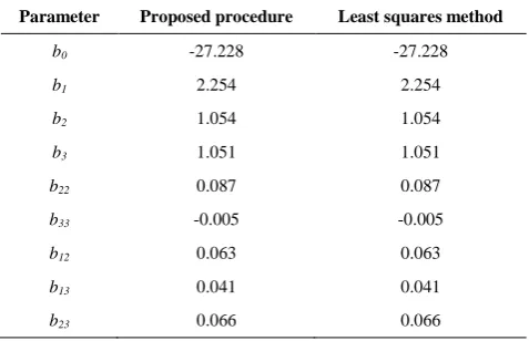
TABLE 4. Comparison between the proposed procedure and

the least squares method for fitting a second-order model to 2142 design

Parameter Proposed procedure Least squares method

b0 -27.228 -27.228

b1 2.254 2.254

b2 1.054 1.054

b3 1.051 1.051

b22 0.087 0.087

b33 -0.005 -0.005

b12 0.063 0.063

b13 0.041 0.041

b23 0.066 0.066

] 5

40 ][ 75 . 0

25 . 5 )[ 24823 . 0 ( -] 5

40 ][ 2

7 [

) 4085 . 0 ( -] 75 . 0

25 . 5 ][ 2

7 )[ 094625 . 0 ( ] 5

40 [

) 1374 . 0 ( -] 75 . 0

25 . 5 )[ 04898 . 0 ( ] 5

40 )[ 11297 . 0 (

-] 75 . 0

25 . 5 )[ 17869 . 0 ( -] 2

7 )[ 9025 . 1 ( 693943 . 6

2 1 2

1

1 1 2

2

2 1 2

1 1

z z z

x

z x z

z z

z x

Y

   

2 1

2 1 1 1 2

2 2 1

2 1 1

066 . 0

041 . 0 063 . 0 005 . 0 -087 . 0

051 . 1 054 . 1 254 . 2 228 . 27

z z

z x z x z

z

z z x Y



 



   

The results of the least squares method and the proposed procedure are given in Table 4 and show that the least squares method and the proposed procedure have the same results. Furthermore, the proposed procedure calculated the coefficients individually, which cannot be performed with the least squares method.

6. CONOCLUSION

Based on the above results and discussion, the proposed procedure for fitting a second-order model to mixed two-level and four-level designs provides fixed formulae regardless of the number of factors, avoids the arduous least squares method, makes it possible to calculate each coefficient individually, and eliminates the need for costly and complicated statistical software.

7. ACKNOWLEDGMENTS

The authors would like to thank the School of Mathematical Sciences, Universiti Sains Malaysia, for providing the facilities.

8. REFERENCES

1. Addelman, S., "Recent developments in the design of factorial experiments", Journal of the American Statistical Association, Vol. 67, No. 337, (1972), 103-111.

2. Davies, O.L., "The design and analysis of industrial experiments", The Design and Analysis of Industrial Experiments, (1954) 234-251.

3. Yates, F., "The design and analysis of factorial experiments",

Imperial Bureau of Soil Science, (1978) 113-125.

4. Margolin, B.H., "Systematic methods for analyzing 2 n ₃ m

factorial experiments with applications", Technometrics, Vol. 9, No. 2, (1967), 245-259.

5. Draper, N.R. and Stoneman, D.M., "Response surface designs for factors at two and three levels and at two and four levels",

Technometrics, Vol. 10, No. 1, (1968), 177-192.

6. Herzberg, A.M. and Cox, D., "Recent work on the design of experiments: A bibliography and a review", Journal of the Royal Statistical Society. Series A (General), (1969), 29-67. 7. Edmondson, R., "Agricultural response surface experiments

based on four-level factorial designs", Biometrics, (1991), 1435-1448.

8. Bisgaard, S., "Accommodating four-level factors in two-level factorial designs", Quality Engineering, Vol. 10, No. 1, (1997), 201-206.

9. Abbas, F.M.A., Low, H.C. and Quah, S.H., "A new method for analyzing experiments of type 2p_{", Proceedings of the National}

Conference on Management Science/Operation Research, (2000), 123-130.

10. Abbas, F.M.A., "A new method for analyzing experiments of type 2p, 3m, and 2p3m", Ph.D thesis, Universiti Sains Malaysia, (2001).

11. Alkarkhi, A.F. and Low, H., "A proposed technique for analyzing experiments of type", Modern Applied Science, Vol. 3, No. 1, (2008), 95-102.

12. Alqaraghuli, W.A., Alkarkhi, A.F. and Low, H., "A new procedure for fitting second-order model to four-level factorial designs", World Applied Sciences Journal, Vol. 22, No. 8, (2013), 1116-1128.

13. Kovo, A., "Application of full 42 factorial design for the development and characterization of insecticidal soap from neem oil", Leonardo Electronic Journal of Practices and Technologies, Vol. 8, No. 1, (2006), 29-40.

14. Hosseinpour, M.N., Najafpoura, G.D., Younesi, H., Khorrami, M. and Vaseghi, Z., "Lipase production in solid state fermentation using aspergillus niger: Response surface methodology", International Journal of Engineering, Vol. 25, No. 3, (2012), 151-159.

15. Kavardi, S.S., Alemzadeh, I. and Kazemi, A., "Optimization of lipase immobilization", International Journal of Engineering,

Transactions A: Basics Vol. 25, No. 1, (2012), 1-9.

16. Yahyaei, M., Bashiri, M. and Garmeyi, Y., "Multicriteria logistic hub location by network segmentation under criteria weights uncertainty" International Journal of Engineering,

Transactions B: Applications Vol. 27, No. 8 (2014) 1205-1214 17. Roger G. P., "Design and analysis of experiment", New York,

Fitting Second-order Models to Mixed Two-level and Four-level Factorial Designs:

Is There an Easier Procedure?

W. A. A. Alqaraghulia_{, A. F. M. Alkarkhi}b _{, H. C. Low} a

a_{School of Mathematical Sciences, Universiti Sains Malaysia, Penang, Malaysia} b_{School of Industrial Technology, Universiti Sains Malaysia, Penang, Malaysia}

P A P E R I N F O

Paper history: Received 29 June 2015

Received in revised form 04 October 2015 Accepted 16 October 2015

Keywords:

Two-level Factorial Design Four-level Factorial Design Response Surface Methodology

هديكچ

شزارب یاهلدم خساپ حطس لاومعم زا هدافتسا اب یرامآ یاه هتسب

تلاداعم لح یارب هدیچیپ

دیلوت روظنم هب دروآرب

بیارض

لدم یم ماجنا .دوش نیا رد هلاقم یارب دیدج شور کی لدم شزارب

خساپ حطس اب حرط طولخم لیروتکاف

حطس ود راهچ و

.دوش یم داهنشیپ حطس و دیدج یاهلومرف

رت ناسآ داهنشیپ یم هبساحم یارب هک دوش مود هجرد ،یطخ

بیارض و لماعت

یارب حرط طولخم لیروتکاف

حطس ود حطس راهچ و زا رظن فرص

لماوع دادعت رد دوجوم

زآ .تسا شیام زا لصاح جیاتن

یداهنشیپ شور اب قفاوت رد

زا لصاح جیاتن تاعبرم لقادح شور

.دشاب یم هلاقم نیا یم ناققحم دناوت ار

هعلاطم یارب

زا هدافتسا ناکما تباث لومرف کی

یارب یاهحرط مامت .دنک بیغرت لیروتکاف