ISSN:0976-3031
Research Article
ESTIMATION OF AUC FOR CONSTANT SHAPE BI-WEIBULL FAILURE
TIME DISTRIBUTION
Leo Alexander, T* and Lavanya, A
Department of Statistics, Loyola College, Chennai–34, India
ARTICLE INFO ABSTRACT
The Receiver Operating Characteristic (ROC) curve is commonly used for evaluating the discriminatory ability of a biomarker. The conventional ways expressing the true accuracy of the test is by using its summary measure Area Under the ROC Curve (AUC) and intrinsic measures Sensitivity and Specificity. We propose a Bayesian approach for the estimation of the AUC under the Constant Shape Bi-Weibull Distribution using Extension of Jeffreys’ Prior Information with three Loss Functions. Theoretical results are validated by simulation studies.Simulations indicated that estimate of AUC values was good even for relatively small sample sizes (n=25). Bayes estimation with General Entropy loss function provides the highest AUC values when the loss parameter is -1.6, according to the extension of Jeffreys prior value is 0.4 or 1.4. When AUC≤0.6, which indicated a marked overlap between the outcomes in diseased and non-diseased populations. An illustrative example is also provided to explain the concepts.
1.
INTRODUCTION
Receiver operating characteristic (ROC) curves are widely used for the evaluation of continuous or ordinal diagnostic tests and biomarkers [6, 7, 22]. Measurements for a diagnostic test may be subject to an analytic limit of detection leading to immeasurable or unreported test results. Ignoring the scores that are beyond the limit of detection of a test leads to a biased assessment of its discriminatory ability, as reflected by indices such as the associated Area Under the ROC Curve (AUC). The ROC Curve is embedded by the two intrinsic measures Sensitivity (Sn) or True Positive Rate (TPR) and 1-Specificity (Sp) or False Positive Rate (FPR) along with its accuracy measure AUC. The corresponding AUC provides a global summary statistic indicating the overall discriminatory ability of a test independent of any cut-off point and may be used to compare the performance of different tests for detection of the condition of interest. The AUC is defined as the total Area under the ROC curve represented by “sensitivity” versus “1-specificity” corresponding to all possible cut-off points. The AUC can be interpreted as the average sensitivity, across all possible False-Positive Fractions [28]. An alternative interpretation is the proportion of the time that test scores for individuals with the condition of interest will exceed (or be less than) those of individuals without the condition. The term ROC analysis was coined during II world war to analyze the radar signals [21]. The application of ROC Curve technique was promoted in diversified fields such as experimental psychology [8], industrial quality control [5] and military monitoring [25]. [8] Was first to use the Gaussian model for estimating the ROC Curve. [3] Gave the maximum likelihood estimates for the ROC Curve parameters considering yes or no type responses and rating data. The importance of ROC Curve in medicine was due to [17] analyze the radiographic images. [19] Proposed a methodology to describe the scores of rating type by embedding the approach of [3]. [10] Explained the importance and robustness of Binormal ROC Curve. Recently [23] explained the Bayesianestimation of the receiver operating characteristic curve for a diagnostic test with a limit of detection in the absence of a gold standard.
We also developed Functional Relationship between Brier Score and Area Under the Constant Shape Bi-Weibull ROC Curve [16], Confidence Intervals Estimation for ROC Curve, AUC and Brier Score under the Constant Shape Bi-Weibull Distribution [13],Asymmetric and Symmetric Properties of Constant Shape Bi-Weibull ROC Curve Described by Kullback-Leibler Divergences [14], and Bayesian Estimation of Parameters under the Constant Shape Bi-Weibull Distribution Using Extension of Jeffreys’ Prior Information with Three Loss Functions [15].
International Journal of
Recent Scientific
Research
International Journal of Recent Scientific Research
Vol. 7, Issue, 10, pp. 13826-13836, October, 2016
Copyright © Leo Alexander, T and Lavanya, A., 2016, this is an open-access article distributed under the terms of the Creative Commons Attribution License, which permits unrestricted use, distribution and reproduction in any medium, provided the original work is properly cited.
Article History:
Received 06th July, 2015
Received in revised form 14th August, 2016 Accepted 23rd September, 2016
Published online 28th October, 2016
Key Words:
Time Distribution
The main purpose of this paper is to compare the traditional Maximum Likelihood Estimation of the AUC of the Constant Shape Bi-Weibull distribution with its Bayesian counterpart using Extension of Jeffreys’ Prior Information obtained from Lindley’s approximation procedure based on three Loss Functions.
In this paper, the Bayesian Estimation of AUC under the Constant Shape Bi-Weibull Distribution is studied by Using Extension of Jeffreys’ Prior Information with Three Loss Functions. This paper is organized as follows: In Section 2, estimation of AUC under MLE, Jeffreys’ Prior Information and Extension of Jeffreys’ Prior Information with Three Loss functions is discussed. Section 3, provides simulation study for proposed theory. Section 4 deals with validation of the proposed theory based on real time data. Conclusions are given in Section 5.
2. A Constant Shape Bi-Weibull Roc Model And Its Auc
In medical science, a diagnostic test result called a biomarker [11, 2] is an indicator for disease status of patients. The accuracy of a medical diagnostic test is typically evaluated by sensitivity and specificity. Receiver Operating Characteristic (ROC) curve is a graphical representation of the relationship between sensitivity and specificity. Hence the main issue in assessing the accuracy of a diagnostic test is to estimate the ROC curve.
Suppose that there are two groups of study subjects: diseased and no diseased. Let S be a continuous biomarker. Assume that ROC analysis based on the True Positive Probability (TPP), ( | ), and False Positive Probability (FPP), ( | ), in fundamental detection problems with only two events and two responses [26,8,4].
According to Signal Detection Theory(SDT), we assume that there are two probability distributions of the random variables X and Y, one associated with the signal event s and other with the non-signal event n[12]; these probability (or density) distributions of a given observation x and y are conditional upon the occurrence of s and n [4].
In the medical context, the signal event corresponds to the diseased group, and the nonsignal event to the no diseased group [9]. If the cutoff value is c, corresponding to a particular likelihood ratio, the TPP and FPP are given by the following expressions [4]:
Let x, y be the test scores observed from two populations with (diseased individuals) and without (no diseased individuals) condition respectively which follow Constant Shape Bi-Weibull distributions. The density functions of Constant Shape Bi-Weibull distributions are as follows,
( | ) =
. (1)
and
( | ) =
. (2)
The probabilistic definitions of the measures of ROC Curve are as follows:
Sensitivity(s ) = ( | ) =
( | )
∞
,
1
Speci icity(s ) = ( | ) =
( | )
.
∞
In this context, the (1-Specificity) and Sensitivity can be defined using equations (1) and (2) and are given in equations (3) and (4) respectively,
( | ) = ( ) =
. (3)
and
( | ) = ( ) =
. (4)
The ROC Curve is defined as a function of (1-Specificity) with scale parameters of distributions and is given as,
where
=
[
( )]
is the threshold and
=
.
The accuracy of a diagnostic test can be explained using the Area under the Curve (AUC) of a ROC Curve.AUC describes the ability of the test to discriminate between diseased and no diseased populations. A natural measure of the performance of the classifier producing the curve is AUC. This will range from 0.5 for a random classifier to 1 for a perfect classifier. The AUC is defined as,
=
( )
( ).
The closed form of AUC is as follows
=
1
1 +
. (5)
2.1 Maximum Likelihood Estimator of AUC
The MLE of two parameters Weibull distribution has been discussed [27] in the context of Reliability estimation. Let X1, X2, .. .… Xm be a random sample of size m from ( , ) and Y1, Y2, .. .… Yn be a random sample of size n from ( , ) .The likelihood function of the selected sample is given by
( ,
| ) =
(
| ,
)
( | ,
) .
where
= ( ,
,
)
′=
The log-likelihood function is
= (
+ )
+ (
1)
+
1
1
, (6)
Differentiating (5) with respect to , we get
=
(
+ )
+
+
1
1
. (7)
By differentiating the equation (5) with respect to , and equating to zero, we get the estimates. The MLE’s of and are determined as,
=
+
∑
=
∑
. (8)
=
+
∑
Time Distribution
Substituting equation (8) and (9) in equation (7) and equating it to zero, we get a non-linear equation:
=
+
+ ∑
+ ∑
∑
∑
+
∑ ∑
. (10)
Hence, can be determined as a solution of Non-linear equation (10). By substituting equations (8), (9) and (10) in equation (5), will get an MLE estimate of AUC and is given as
=
1
1 +
,
=
.
2.2 Bayesian Estimation of AUC under Constant Shape Bi-Weibull Distribution
Bayesian Estimation approach has received a lot of attention in recent times for analyzing Failure Time data, which has mostly been proposed as an alternative to that of the traditional methods.
Bayesian Estimation approach makes use of once prior knowledge about the parameters as well as the available data. When once prior knowledge about the parameter is not available, it is possible to make use of the non-informative prior in Bayesian analysis.
Since we have no knowledge of the parameters, we seek to use the Extension of Jeffreys’ Prior Information, where Jeffreys’ Prior is the square root of the determinant of the Fisher information. According to [1], the extension of Jeffreys’ prior is by taking u(θ) ∝ [I(θ)], cϵR , so that
( ) ∝
1
Thus,
( , ) ∝
1
.
Let X1, X2, .. .… Xm be a random sample of size m from ( , ) and Y1, Y2, .. .… Yn be a random sample of size n from ( , ) .The likelihood function of the selected sample is given by
( ,
| ) =
(
| ,
)
( | ,
) .
where
= ( ,
,
)
′=
.
With Bayes theorem, the joint posterior distribution of the parameters is
π
( |t) ∝ L(t| )u( )
=
(
)
,
wherekis the normalizing constant that makes a proper pdf.
Remark 2.1
Here we consider two Asymmetric Loss Functions namely Linear Exponential (LINEX) Loss Function and General Entropy Loss Function. Also the Symmetric Loss Function namely Squared Error Loss Function considered in order to estimate AUC values.
2.2.1 Linear Exponential Loss Function (LINEX)
L
θ
θ
∝ exp a
θ
θ
a
θ
θ
1
where is an estimation of θ and a ≠ 0. The sign and magnitude of the shape parameter ‘a’ represents the direction and degree of symmetry, respectively. There is overestimation if a>0 and underestimation if a<0 but when 0 , the LINEX Loss Function is approximately the Squared Error Loss Function. The posterior expectation of the LINEX Loss Function, according to [20], is
∝
(exp(
))
( )
1 . (11)
The Bayes Estimator of θ, represented by under LINEX Loss Function, is the value of which minimizes equation (11) and is given as
=
1
(
(
)).
Provided ( ( )exists and is finite. The Bayes Estimator of a function
= (
(
),
(
) ,
(
))
is given as
= (exp (
),
(
) ,
(
) | )
=
∬ [
(
),
(
) ,
(
)] ( )
∬
(
,
, )
. (12)
From (12), it can be observed that ratio of integrals which cannot be solved analytically and for that we employ Lindley’s approximation procedure to estimate the parameters. Lindley considered an approximation for the ratio of integrals for evaluating the posterior expectation of an arbitrary function ( ) as
[ ( )| ] =
∫ ( ) ( )[ ( )]
∫ ( )[ ( )]
.
According to [24], Lindley’s expansion can be approximated asymptotically by
=
+
1
2
[
+
+
] +
+
+
+
1
2
+
+
, (13)
whereL is the log-likelihood function in equation (6),
(
) =
(
),
=
=
(
),
=
=
(
),
=
=
=
= 0,
(
) =
(
) ,
=
=
(
),
=
=
(
),
=
=
=
= 0
( ) =
(
)
,
=
=
(
)
,
Time Distribution
(
,
, ) =
(
)
(
)
(
),
=
=
1
,
=
=
1
,
=
=
1
,
= (
) ,
= (
) ,
= (
) ,
=
=
1
(
)
1
,
=
= 2
1
(
) + 2
1
,
=
=
2
∑
,
=
=
2
∑
,
=
=
2
+ 6
∑
,
=
=
2
+ 6
∑
.
Bayesian Estimation of AUC using LINEX Loss Function is given as
=
1
1 +
,
=
2.2.2 General Entropy Loss Function
Another useful Asymmetric Loss Function is the General Entropy (GE) Loss which is a generalization of the Entropy Loss and is given as
L
θ
θ
∝
θ
θ
1 .
The Bayes Estimator of θunder the General Entropy Loss is
=[
(
)] ,
provided
(
)
exists and is finite.
The Bayes Estimator for this Loss Function is
= { [
,
,
]| }
=
∬ [
,
,
]
(
,
, )
Applying the same Lindley approach here as in (13) with u100, u200, u010, u020 and u001, u002 are the first and second derivatives for , and β, respectively, and are given as
= [
],
=
=
[
] ,
=
=
(
)
,
=
=
=
= 0,
= [
],
=
=
[
] ,
=
=
(
)
,
=
=
=
= 0,
= [
],
=
=
[
],
=
=
(
)
,
=
=
=
= 0.
Bayesian Estimation of AUC using the General Entropy Loss is given as
=
1
1 +
,
=
.
2.2.3 Symmetric Loss Function
The Squared Error Loss is given by
L
θ
θ
∝
θ
θ .
This Loss Function is symmetric in nature, that is, it gives equal weightage to both over and under estimation.
In real life, we encounter many situations where overestimation may be more serious than underestimation or vice versa.
The Bayes Estimator of a function = ( , , )of the unknown parameters under Square Error Loss Function (SELF)is the posterior mean, where
= { [
,
, ]| } =
∬ [ , ]
(
,
, )
∬
(
,
, )
.
Applying the same Lindley approach here as in (13) where
u
100,
u
200,
u
010,
u
020 and
u001
,
u002
are the
first and second derivatives for
,
and
β
, respectively, and are given as
=
,
=
= 1,
=
=
=
=
= 0,
=
,
=
= 1,
=
=
=
=
= 0,
Time Distribution
=
=
=
=
= 0.
Bayesian Estimation of AUC using The Squared Error Loss is given as
=
1
1 +
,
=
.
3. Simulation Study
Simulation studies are conducted with different combinations of scale and shape parameters of both diseased and non-diseased populations. At every parameter combination and sample size, the AUC is obtained. The main purpose of conducting simulations is to show how the AUC of ROC curve possesses different values as the scale and shape parameters of the normal and abnormal distributions change.
The AUC has been computed through different methods via MLE and Bayesian Estimation using Extension of Jeffreys’ Prior Information obtained from Lindley’s approximation procedure with three Loss Functions.
In our Simulation study, we chose a sample size of n=25, 50, and 100 to represent small, medium, and large dataset. The assumed scale and shape parameters of both populations are = = 0.5 and 1.5, = 0.8 and 1.2. The values of Jeffreys’ Extension are
= 0.4 and 1.4. The values for the Loss parameters (a, k) are a=k=±0.6 and ±1.6.
In Table 1 we present the estimated values for AUCfor both the Maximum Likelihood Estimation and Bayesian Estimation using anextension of Jeffrey’s prior information with the three loss functions.
From Table 1 it is observed that Bayes estimator under LINEX and General Entropy Loss functions tends to underestimate the AUC values when loss parameters value are (0.6,1.6).
Bayes estimation with General Entropy loss function provides the highest AUC values when the loss parameter is -1.6, according to the extension of Jeffreys prior value is 0.4 or 1.4. So that the Bayes estimators of AUC under General Entropy loss function is best estimation method for Constant Shape Bi-Weibull Distribution.
4. Illustration
The real data set namely Coronary Heart Disease [CHDAGE] Data extracted from [29].Data consists of 100 Observations, 3 variables. For this data, we have to find estimated AUC values. This data consists of patients who are Diseased and who are Non-diseased. We have to know the patients with Diseased and patients without Diseased and age is most influential variable for diagnose. Table 2 depicts the Estimated AUC values using CHDAGEData.
Table 1 Estimated values for AUC
(m, n) β c
a=k=0.6 a=k=-0.6 a=k=1.6 a=k=-1.6
(25,25) 1.5 1.5 1.5 1.5 0.5 0.5 0.5 0.5 0.8 1.2 0.8 1.2 0.4 1.4 0.4 1.4 0.6518 0.6492 0.6620 0.7641 0.7641 0.7629 0.7734 0.7777 0.3251 0.3276 0.3271 0.3283 0.3352 0.3360 0.3266 0.3199 0.6588 0.6574 0.6620 0.6628 0.6684 0.6675 0.6757 0.6798 0.0961 0.1019 0.1095 0.1144 0.1438 0.1446 0.1299 0.1193 0.8353 0.8339 0.8459 0.8495 0.8693 0.8681 0.8778 0.8800 (50,50) 1.5 1.5 1.5 1.5 0.5 0.5 0.5 0.5 0.8 1.2 0.8 1.2 0.4 1.4 0.4 1.4 0.7482 0.8011 0.7402 0.7529 0.7494 0.7423 0.7585 0.7648 0.3510 0.3535 0.3468 0.3402 0.3414 0.3446 0.3350 0.3301 0.6460 0.6437 0.6505 0.6551 0.6586 0.6540 0.6652 0.6699 0.1584 0.1626 0.1521 0.1387 0.1478 0.1507 0.1387 0.1319 0.8287 0.8251 0.8364 0.8414 0.8523 0.8438 0.8619 0.8681 (100,100) 1.5 1.5 1.5 1.5 0.5 0.5 0.5 0.5 0.8 1.2 0.8 1.2 0.4 1.4 0.4 1.4 0.7063 0.8021 0.6719 0.8078 0.7509 0.7466 0.7561 0.7556 0.3511 0.3539 0.3478 0.3502 0.3408 0.3425 0.3372 0.3360 0.6467 0.6448 0.6498 0.6487 0.6596 0.6569 0.6633 0.6634 0.1597 0.1655 0.1540 0.1597 0.1473 0.1485 0.1424 0.1393 0.8308 0.8289 0.8356 0.8354 0.8541 0.8489 0.8598 0.8583 ML: Maximum Likelihood, BS: Squared Error Loss function, BL: LINEX Loss function, BG: General Entropy Loss function
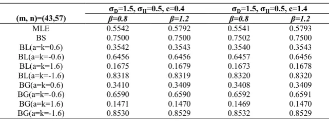
Table 2 Estimated AUC values using CHDAGE Data
(m, n)=(43,57)
=1.5, =0.5, c=0.4 =1.5, =0.5, c=1.4
β=0.8 β=1.2 β=0.8 β=1.2
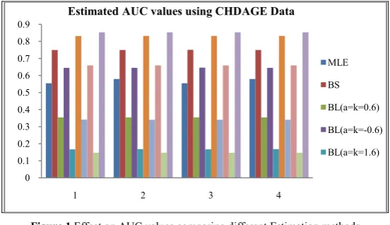
From Table 2, we observe that Bayes estimation with General Entropy loss function provides the highest AUC values when the loss parameter is -1.6, according to the extension of Jeffreys prior value is 0.4 or 1.4. So that the Bayes estimators of AUC under General Entropy loss function is best estimation method for Constant Shape Bi-Weibull Distribution using CHDAGE Data.
To demonstrate the proposed methodology with the help of graphical visualization, Figures 1 is drawn for comparing the Estimated AUC values under Constant Shape Bi-Weibull distribution using CHDAGE Data.
From Figure 1, it is visualized that Bayes estimation with General Entropy loss function provides the highest AUC values when the loss parameter is -1.6.
5.
CONCLUSION
The main objective of this paper is Bayesian estimation of AUC for the Constant Shape Bi-Weibull distribution, under three Loss functions, namely, the Linear Exponential (LINEX) Loss, General Entropy Loss, and Square Error Loss functions. Also,The Maximum Likelihood Estimation of AUC is discussed. Bayes estimators were obtained using Lindley approximation while MLE was obtained using Newton-Raphson method.
A Simulation study was conducted to examine and compare the performance of the estimators for different sample sizes with different values for the extension of Jeffreys’ prior and the loss functions.
We also observe that Bayes estimation with General Entropy loss function provides the highest AUC values when the loss parameter is -1.6, according to the extension of Jeffreys prior value is 0.4 or 1.4.
So that the Bayes estimators of AUC under General Entropy loss function is best estimation method for Constant Shape Bi-Weibull Distribution.
References
1. Al-Kutubi, H.S., Ibrahim, N.A., 2009, Bayes estimator for exponential distribution with extension of Jeffery prior information, Malaysian Journal of Mathematical Sciences3(2), 297–313.
2. Betinec, M., 2008, Testing the difference of the ROC curves in biexponential model, Tatra Mt. Math. Publ39, 215-223. 3. Dorfman., Alf., 1969, Maximum – Likelihood Estimation of parameters of signal detection theory and determination of
confidence interval–rating method data, Journal of Mathematical Psychology6, 487-496.
4. Dorfman, D.D., Berbaum, K.S., Metz, C.E., Lenth, R.V., Hanley, J.A., Dagga, H.A., 1996, Proper receiver operating characteristic analysis: the bigamma model, Acad. Radiol4, 138-149.
5. Drury, C.G., Fox, J.G., 1975, Human reliability in quality control, Halsted, New York.
6. Gardner, I.A., Greiner, M., 2006, Receiver-operating characteristic curves and likelihood ratios: improvements over traditional methods for the evaluation and application of veterinary clinical pathology tests, Veterinary Clinical Pathology 35(1), 8-17.
7. Greiner, M.D., Smith, R.D., 2000, Principles and practical application of the receiver operating characteristic analysis for diagnostic tests, Preventive Veterinary Medicine45(1–2), 23-41. DOI: 10.1016/S0167-5877(00)00115-X.
8. Green, D.M., Swets, J.A., 1966, Signal Detection Theory and Psychophysics, John Wiley and Sons Inc, New York, NY, USA.
9. Hanley, J.A., Mc Neil, B.J., 1982, A Meaning and use of the area under a Receiver Operating Characteristics (ROC) Curves, Radiology143, 29-36.
10. Hanley, J.A., 1988, The Robustness of the Binormal Assumption used in fitting ROC curves, Medical Decision Making8,197-203.
11. Hanley, J.A., et al., 1989, Receiver Operating Characteristic (ROC) methodology: the state of the art, Critical Reviews in Diagnostic Imaging29(3), 307-335.
Figure 1 Effect on AUC values comparing different Estimation methods
0 0.1 0.2 0.3 0.4 0.5 0.6 0.7 0.8 0.9
1 2 3 4
Estimated AUC values using CHDAGE Data
MLE
BS
BL(a=k=0.6)
BL(a=k=-0.6)
Time Distribution
12. Hughes, G., Bhattacharya, B., 2013, Symmetry Properties of Bi-Normal and Bi-Gamma Receiver Operating Characteristic Curves are described by Kullback-Leibler Divergences, Entropy15, 1342-1356.
13. Lavanya, A., Leo Alexander, T., 2016, Confidence Intervals Estimation for ROC Curve, AUC and Brier Score under the Constant Shape Bi-Weibull Distribution, International Journal of Science and Research 5(8), 371-378.
14. Lavanya, A., Leo Alexander, T., 2016, Asymmetric and Symmetric Properties of Constant Shape Bi-Weibull ROC Curve Described by Kullback-Leibler Divergences, International Journal of Applied Research 2(8), 713-720.
15. Lavanya, A., Leo Alexander, T., 2016, Bayesian Estimation of Parameters under the Constant Shape Bi-Weibull Distribution Using Extension of Jeffreys’ Prior Information with Three Loss Functions, International Journal of Science and Research5(9), 96-103.
16. Leo Alexander, T., Lavanya, A., 2016, Functional Relationship between Brier Score and Area Under the Constant Shape Bi-Weibull ROC Curve, International Journal of Recent Scientific Research7(7), 12330-12336.
17. Lusted, L.B., 1971, Signal detectability and medical decision making, Science 171,1217-1219.
18. Metz, C.E., 1989, Some practical issues of experimental design and data analysis in radiological ROC studies, Invest Radiol24, 234-245.
19. Metz, C.E., Herman, B.E., Shen, J.H., 1998, Maximum likelihood estimation of receiver operating characteristic (ROC) curves from continuously distributed data, Statistics in Medicine17(9), 1033-1053.
20. Pandey, B.N., Dwividi, N., Pulastya, B., 2011, Comparison between bayesian and maximum likelihood estimation of the scale parameter in Weibull distribution with known shape under linex loss function, Journal of Scientific Research55, 163– 172.
21. Peterson, W.W., Birdsall, T.G., Fox, W.C., 1954, The theory of signal detectability, Transactions of the IRE Professional Group on Information Theory, PGIT2(4),171-212.
22. Pepe, M.S., 2003, The Statistical Evaluation of Medical Tests for Classification and Prediction, Oxford University Press: New York, NY.
23. Seyed Reza Jafarzadeha., Johnsonb, W.O., Uttsb, J.M., Gardnera, I.A., 2010, Bayesian estimation of the receiver operating characteristic curve for a diagnostic test with a limit of detection in the absence of a gold standard, Statist. Med29, 2090— 2106.
24. Sinha, S.K., 1986, Bayesian estimation of the reliability function and hazard rate of a Weibull failure time distribution, Tranbajos De Estadistica1(2), 47–56.
25. Swets, J.A., Egilance., 1977, Relationships among theory, Physiological correlates and operational performance, Plenum, New York.
26. Swets, J.A., Pickett, R.M., 1982, Evaluation of Diagnostic Systems: Methods from Signal Detection Theory, Academic Press, New York.
27. Zhou, S.H., Obuchowski, N.A., McClish DK., 2002, Statistical Methods in Diagnostic Medicine, New York, NY: John Wiley & Sons, Inc.
28. Zweig, M.H., Campbell, G., 1993, Receiver operating characteristic (ROC) plots: a fundamental evaluation tool in clinical medicine, Clinical Chemistry39(4), 561--577.
29. https://www.umass.edu/statdata/statdata/data/chdage.txt
*******