Hyperparameter Optimization on Neural Machine Translation

Spring 2019

Hyperparameter Optimization on Neural Machine Translation

Hyperparameter Optimization on Neural Machine Translation

Souparni Agnihotri

Iowa State University, [email protected]

Follow this and additional works at: https://lib.dr.iastate.edu/creativecomponents

Part of the Artificial Intelligence and Robotics Commons

Recommended Citation Recommended Citation

Agnihotri, Souparni, "Hyperparameter Optimization on Neural Machine Translation" (2019). Creative Components. 124.

https://lib.dr.iastate.edu/creativecomponents/124

by

Souparni Agnihotri

A Creative Component submitted to the Graduate Faculty

in partial fulfillment of the requirements for the degree of

MASTER OF SCIENCE

Major: Computer Engineering

Program of Study Committee: Chinmay Hegde, Major Professor

The student author, whose presentation of the scholarship herein was approved by the program of study committee, is solely responsible for the content of this dissertation/thesis. The Graduate College will ensure this dissertation/thesis is globally accessible and will not permit alterations

after a degree is conferred.

Iowa State University

Ames, Iowa

2019

TABLE OF CONTENTS

Page

LIST OF TABLES . . . v

LIST OF FIGURES . . . vi

ACKNOWLEDGMENTS . . . vii

ABSTRACT . . . viii

CHAPTER 1. OVERVIEW . . . 1

1.1 Introduction . . . 1

CHAPTER 2. REVIEW OF LITERATURE . . . 3

2.1 Recurrent Neural Networks . . . 3

2.2 Encoder Decoder Model . . . 4

2.3 Vanishing Gradient Decent . . . 5

2.4 Long Short Term Memory Networks . . . 5

2.5 The Transformer . . . 6

2.6 ELMo . . . 8

2.7 BERT . . . 8

2.8 Sequence to Sequence Learning with Neural Networks . . . 9

2.9 Hyper parameter Optimization . . . 10

CHAPTER 3. METHODS AND PROCEDURES . . . 11

3.1 Introduction . . . 11

3.2 Hyperparameter selection . . . 11

3.2.1 Learning Rate . . . 11

3.3.1 Stochastic Gradient Descent . . . 12

3.3.2 Adam Optimizer . . . 12

3.4 Type of attention . . . 12

3.4.1 Bahdanau . . . 13

3.4.2 Luong . . . 13

3.5 Attention Architecture . . . 13

3.5.1 Standard . . . 13

3.5.2 Google Neural Machine Translation (GNMT) . . . 13

3.6 Encoder type . . . 14

3.6.1 Unidirectional . . . 14

3.6.2 Regularization . . . 15

3.7 Inference mode . . . 15

3.7.1 Greedy . . . 15

3.7.2 Beam Search . . . 16

3.8 Testing mechanism . . . 17

3.8.1 BLEU scores . . . 17

3.9 Random Search . . . 17

3.10 Successive Halving . . . 17

3.11 Hyperband . . . 18

CHAPTER 4. RESULTS . . . 20

4.1 System Configurations: . . . 20

4.2 Training Data: . . . 20

4.3 Evaluation . . . 20

CHAPTER 5. SUMMARY AND DISCUSSION . . . 26

LIST OF TABLES

Page

4.1 The different hyperparameter configurations obtained via random search . . 21

4.2 The different hyperparameter configurations obtained via random search . . 21

4.3 The different hyperparameter configurations obtained via successive halving 22

LIST OF FIGURES

Page

2.1 Architecture of an RNN . . . 3

4figure.14 6figure.17 7figure.19 3.1 Bi-directional RNNs (http://opennmt.net/OpenNMT) . . . 15

16figure.45 4.1 The variation of the BLEU for every step in the training process . . . 23

4.2 The variation of the BLEU score obtained with respect to different learning rates. The congiguration used was . . . 24

4.3 Vietnamese to English translations . . . 24

4.4 Vietnamese to English translations . . . 25

4.5 German to English translation at epoch 122000 . . . 25

ACKNOWLEDGMENTS

I would like to take this opportunity to express my thanks to Dr. Chinmay Hegde for his help

during the various aspects of conducting research and the writing of this thesis. His guidance,

patience and support were invaluable throughout my degree, and his insights and words of

ABSTRACT

With the growth of deep learning in the recent years, there have been several models created to

tackle different real world goals, autonomously. One such goal is the automatic translation of text

from one language to another. This is commonly known as Neural Machine Translation (NMT).

NMT has proved to be a significant challenge to achieve, given the fluidity of human language.

Most NMT models rely on Recurrent Neural Networks (RNNs) and deep Long Short-Term

Memory networks (LSTMs). In this study, we will explore the Sequence to Sequence Learning with

Neural Networks Model (Sutskever et al. (5)) and perform an ablation study of the model on two

different data sets - the English-Vietnamese parallel corpus by the IWSLT Evaluation Campaign,

CHAPTER 1. OVERVIEW

In the recent years, Neural Machine Translation (NMT) has seen immense growth. In this

report, we introduce Neural Machine Translation and the major concepts associated with it.

Ar-chitectures such as Recurrent Neural Network (RNN), Long Short term Memory Networks (LSTM),

the Transformer, Sequence to Sequence learning with Neural Networks and the Google Neural

Ma-chine Translation model (GNMT) are crutial for understanding NMT in detail. We then explain

the hyperparameters that can be tuned to make the Machine Translation Model better and discuss

different ways to find the right hyperparameter configuration for a given dataset. We show the

results obtained from our experiments and the inferences that can be gained from them. This

report will provide insight to training and testing of future NMT models.

1.1 Introduction

Neural Machine Translation has generated a lot of interest in solving the Machine Translation

problem in the recent years. The use of Deep Neural Networks (DNNs) has proved extremely

powerful because of their ability to perform arbitrary parallel computation within a small number

of steps. In addition, DNNs support supervised backpropogation so that when they are trained with

enough information, supervised backpropogation might find the optimal parameters to solve the

problem. However, one of the biggest limitations of DNNs is that it can only be applied to problems

whose inputs and outputs can be sensibly encoded with vectors of the same dimensionality. To solve

this issue, LSTMs are introduced. One of the useful properties of LSTMs is that they can learn to

map an input sentence of variable length into a fixed dimensional vector representation, Translations

tend to be paraphrases of the input sentence and the translation objective encourages LSTMs to

find sentence representations that capture their meaning as sentences with similar meanings will

For this study, we use the seq2seq model provided by Neural Machine Translation (seq2seq)

tutorial (Luong et al. (9)) which uses an encoder-decoder mechanism to generate the machine

translations. We compare and contrast the workings of different hyperparameters on the two

CHAPTER 2. REVIEW OF LITERATURE

2.1 Recurrent Neural Networks

Recurrent Neural Networks are networks in which information is propagated from the previous

time step to the next time step. They can be thought of as multiple copies of the same network,

each passing a message from one successor to another. This chain-like structure suggests that RNNs

can be associated with sequences or lists and have thus found a variety of applications like speech

recognition, language processing and machine translation.

RNNs simply accept an input sequence x and output a sequence y. The crucial factor is that that

the output’s vector is influenced not only by the corresponding input, but by the whole sequence

of inputs that has been fed in. RNNs can be shaped as a form of repeating modules of a neural

network. The repeating module contains a single simple structure – such as that of a single tanh

layer as shown below.

Figure 2.1 Architecture of an RNN

When an RNN takes a sentence in as an input, it handles the sentence word by word. This

are long, the model is prone to forgetting the content of distant positions as described insection 2.3.

All these issues are solved with the introduction of the transformer architecture insection 2.5.

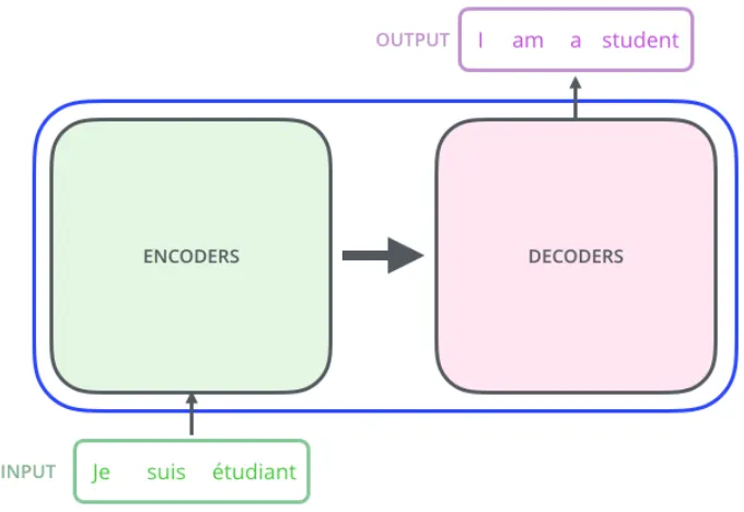
2.2 Encoder Decoder Model

One of the most common types of architectures used for machine translation is the

encoder-decoder model. The encoder - true to its name - encodes the sequence to a fixed dimensional vector.

The decoder then processes this vector to produce a translation.

Figure 2.2 Depiction of the Encoder Decoder Model taken from ”The Illustrated Trans-former”.Alammar Jay. (13)

One of the key benefits to such a model is the ability to handle variable length input and

output sentences of text. Later in the report, we will see when encoder decoder models were first

2.3 Vanishing Gradient Decent

In language modeling, there are cases where there is a need to store very long-term dependencies.

Suppose we have to predict the last word in the sentence ”I live in Germany and I speak fluent

German.” We need the context of Germany to predict the word German. There is a chance that

the gap between the relevant information and the point where it is needed becomes very large.

The shortcomings of RNNs shows up when they are no longer able to connect the long term

dependencies.

This was further explored in the paper ”Learning Long-Term Dependencies with Gradient

Descent is Difficult” Bengio et al (1). As the context length between two words increases, layers in

the unrolled RNN also increase. As the network becomes deeper the gradients flowing back in the

back propagation step becomes smaller. As a result, the learning rate becomes very slow and makes

it infeasible to expect long term dependencies for that language. As a result, RNNs face difficulty

in memorizing previous words very far away in the sequence and can only make predictions based

on the recent words.

Long Short Term Memory Networks (LSTMs) solve this issue.

2.4 Long Short Term Memory Networks

LSTMs are a special kind of RNN capable of learning long-term dependencies. They are

ex-plicitly designed to solve the vanishing gradient problem.

They differ from regular RNNs in that the recurring/repeating module has a different structure.

Instead of a single neural network layer, there are 4 layers interacting with each other. The LSTM

maintains a cell state that carries the information across it. The LSTM has the ability to add or

remove information to the cell state through carefully regulated structures called gates. Gates are

composed out of a sigmoid neural net layer and a pointwise multiplication operation. This way,

they have the ability to optionally let information through. This layer is also called the ”forget

The second step is to decide what information is going to be stored in the cell state. First, a

sigmoid layer decides which values are going to be updated and a tanh layer creates a vector of

candidate values that would be added to the state. Both these values are combined to create an

updated version of the cell state.

The final step decides what is going to be the output. First, a sigmoid layer is run to decide

which parts of the cell state is going to be in the output. Then this cell state is put through tanh

and multiply the output of the sigmoid gate. This will ensure that the output will contain only the

parts we want it to contain.

Figure 2.3 LSTM picture taken from(author?) (LSTM- Colah’s blog)

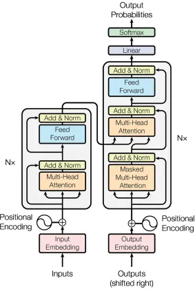
2.5 The Transformer

The Transformer is a model that uses attention to speed up the training of attention networks.

They allow for significantly more parallelization and thus solves the regular problems faced by

RNNs. The Transformer follows the overall architecture of the encoder decoder model by using

stacked attention and point wise fully connected layers for both the encoder and the decoder.

The encoding component has a stack of encoders on top of each other and the decoding

com-ponent also has a stack of decoders of the same length. Each of the encoders is broken down into

applied to the feed forward neural network. The decoder is composed of both those layers but has

an attention layer in between them to focus on relevant parts of the sentence.

The architecture of the Transformer is as follows:

2.6 ELMo

Over the last one year, a new type of deep contextualized word representation was introduced

that models the complex characteristics of word use as well as how these uses vary across linguistic

contexts. According to the ”Deep Contextualized Word Representations” paper, these word

em-beddings are learned functions of the internal states of a deep bidirectional language model (biLM),

which is pre-trained on a large text-corpus.

The three salient ELMo representations are:

• Contextual - The representation of each word depends on the entire context in which it is

used.

• Deep - The word representations combine all the layers of a deep pre-trained neural network

• Character based - ELMo representations are purely character based, allowing the network to

use morphological clues to form robust representations for out-of-vocabulary tokens unseen

in training.

It has been found that adding ELMo to existing NLP systems has significantly improved the state

of the art for every considered task. The above information was referred from Peters et al. (11)

2.7 BERT

Bidirectional Encoder Representations from Transformers (BERT) is a recent approach

pub-lished in Devlin et al. (12). It is designed to pre-train bidirectional representations of Transformer

and apply it to language modeling. The paper shows that a language model which is bidirectionally

trained can have a deeper sense of language context and flow than uni directional models. Since

BERTs main goal is to generate a language model, it only uses the encoder mechanism of the

Transformer. The specifics of the BERT model can be obtained from the paper. BERT can be

• Classification tasks can be carried out by adding a classification layer on top of the

Trans-former output

• Using BERT, Question Answering models can be trained by learning two extra vectors that

mark the beginning and the end of an answer.

It has been shown that using BERT has provided state of the art results on a wide variety of

Natural Language Processing (NLP) tasks. BERT has proven to be a breakthrough in Machine

Learning and NLP. Its approchability and fast fine-tuning allows for a wide range of applications.

2.8 Sequence to Sequence Learning with Neural Networks

Sequence to Sequence Learning with Neural Networks was introduced in 2014. The paper

introduced an end to end to sequence learning. Their method used a multilayered LSTM to map

the input sequence to a vector of fixed dimensionality and then another deep LSTM to decode the

target sentence from the vector. The paper, ”Sequence to Sequnce Learning with Neural Networks”

Sutskever et al. (5) specifically tackles the translation of English to French on the WMT14 dataset.

Although LSTMs have been developed to do machine translation, the authors approach had some

major modifications that built on top of regular LSTMs. One of the things LSTMs suffer from

is their performance on very large sentences as even they tend to forget some very long term

dependencies. One of the major modifications the authors made, was that they reversed the order

of words in the source sentence but not the target sentence in the training and test set. By doing so,

they introduced many short term dependencies that made the optimization problem much simpler.

For example, given an input sequence a, b, c and it had to be translated to x, y and z , the LSTM

was asked to map c, b, a to x, y and z instead of doing a direct mapping. This way, a would be in

close proximity with x, b in close proximity y with and so on.

Their overall model differed from a regular LSTM in the fact that they used two different

LSTMs. The first LSTM is used to read the input sequence and obtain a large fixed dimensional

vector representation. The second LSTM, which is essentially a RNN language model conditioned

increases the number of model parameters at negligible computational cost, making it natural to

train on multiple language pairs simultaneously. In addition to the above, the authors used a deep

LSTM of four layers as they found that it significantly outperforms shallow LSTMs.

A fascinating result of this approach is that the source sentences were reversed. The authors

found that doing so increased the BLEU scores from 25.9 to 30.6. They believe this is because of

the introduction of many short term dependencies. In general, when a source sentence and target

sentence is concatenated together, each word in the source sentence is very far away from the target

sentence. But when the source sentence is reversed, the average distance between the corresponding

words in the source and target language remain unchanged. Since the first few words in the source

sentence are very close to the first few words in the target sentence, back propagation could have

an easier time finding the sequence and communicating with the source and target sentence which

results in overall improvement in performance.

2.9 Hyper parameter Optimization

While training a model, it is important to know which hyperparameters to choose.

Hyperpa-rameters refer to the paHyperpa-rameters that are set before the start of training. The time required to

train and test a model is dependent on the types of hyperparameters chosen. The tune-ability of an

algorithm, hyperparameter, or interacting hyperparameters is a measure of how much performance

can be gained by tuning it. For an LSTM, the learning rate followed by the network size are its most

crucial hyperparameters. Hyperparameter optimization relies on finding the most optimal tuple

which will minimize the predefined loss function on a given data. In this paper we will specifically

analyze which hyperparameters work best on the NMT models – specifically the model inspired by

CHAPTER 3. METHODS AND PROCEDURES

3.1 Introduction

The basis for hyperparameter optimization lies in picking the right hyperparameters before

training. Once these hyperparameters are picked, it is important to narrow down our options so

that we end up with a certain configuration that would work on our given model and dataset.

This section introduces the different hyperparameters that were chosen and the algorithms used to

narrow down the list so as to obtain the most optimal hyperparameters for the given NMT task.

3.2 Hyperparameter selection

3.2.1 Learning Rate

The learning rate is a hyperparameter that controls how much the weights of the network are

getting adjusted with respect to the loss gradient. Typically learning rates are configured at random

by the user. It is often hard to get it right. The way in which learning rate changes over time

(training epochs) is referred to learning rate decay, ”Adaptive learning rate” is a process in which a

small learning rate is chosen and if the performance doesn’t improve after a fixed number of epochs,

the learning rate is increased by a fixed number tested again. An adaptive learning rate generally

outperforms a model with a badly configured learning rate.

3.3 Optimizer

An optimizer is a mathematical way of measuring how wrong the predictions are, Optimizers

tie together the loss function and the model parameters by updating the model in response to the

output of the loss function. There are two types of optimizers we will discuss - Stochastic Gradient

3.3.1 Stochastic Gradient Descent

Gradient descent is an algorithm that has been used all across Machine Learning to optimize.

There are three steps involved in gradient descent –

• Calculate what a small change in each individual weight would do to the loss function

• Adjust each individual weight based on its gradient.

• Repeating the first two steps until loss is minimized

It is important to find the right learning rate so as to avoid the gradient from getting stuck in

a local minima.

In Stochastic gradient descent, instead of calculating the gradients of all of our training examples

on every pass of the gradient, we only use a small subset or mini-batches of training examples. The

reason this is done is to first reduce the variance in parameter update and hence, lead to a more

stable convergence; and second, to utilize highly optimized matrix operations that should be used

for computing the cost and gradient.

3.3.2 Adam Optimizer

Adam stands for adaptive moment estimation. Adam utilizes the concept of momentum by

adding fractions of previous gradients to the current one. We are not going to go into the

math-ematics of this here but it is important to remember that all optimizers have the same goal:

minimizing the loss function.

3.4 Type of attention

This describes the type of attention mechanism that we use in the encoder and decoder. More

3.4.1 Bahdanau

This mechanism gives decoder a way to ”pay attention” to parts of the input rather than

relying on a single vector. Attention is calculated with a feedforward layer in the decoder which

then creates a new vector which is processed through a softmax layer to create attention weights

that are multiplied with encoders outputs to create a new context vector which is used to predict

the next output. The attention scores in Bahdanau are calculated using the concat mechanism

which involves taking a dot product between a new parameter va and a linear transform of the

states concatenated together.

3.4.2 Luong

The Effective Approaches to Attention-based Neural Machine Translation introduced by Luong

et al. describes a few more attention models that offer improvements and simplification. The main

difference between the luong attention and the bahdanau mechanism is the scoring. In luong, the

specific score function that compares two states is a dot product between the current states and

the previous hidden state of the network.

3.5 Attention Architecture

3.5.1 Standard

The standard attention architecture refers to the architecture described in sequence to sequence

learning with neural networks (section 2.8)

3.5.2 Google Neural Machine Translation (GNMT)

The GNMT model described by Wu et al. (7) aims to address the issue that NMT systems

lack robustness, particularly when the input sentences contain rare words. The model consists of

a deep LSTM network with 8 encoder and 8 decoder layers using residual connections as well as

bottom layer of the decoder to the top layer of the encoder in an attempt to improve parallelism

and decrease training time. In the GNMT model, the words are divided into a limited set of

sub-word units in order to handle rare sub-words. According to the paper, this method provides a good

balance between the flexibility of character-delimited models and the efficiency of word-delimited

models, naturally handles translation of rare words, and ultimately improves the overall accuracy

of the system. In addition, their beam search technique employs a length-normalization procedure

and uses a coverage penalty, which encourages generation of an output sentence that is most likely

to cover all the words in the source sentence. This architecture has achieved state of the art

performance on the EMT’14 English-to-French and English-to-German datasets.

3.6 Encoder type

3.6.1 Unidirectional

A unidirectional encoder is a simple recurrent neural network. (LSTM) The unidirectional

LSTM only preserves information from the past as the inputs it gets are only from the past.

3.6.1.1 Bi-directional

The bidirectional encoder consists of two independent encoders. One for the encoding of the

normal sequence and another for the encoding for the reversed sentence. Hence, the input is run

two ways – one from the past to the future and another from the future to the past. The output

and final states are concatanated or summed. Using the two hidden states, we can, at any point in

time, preserve the information from both the past and the future.

The figure 3.1 illustrates the past and the future states interacting with each other.

3.6.1.2 GNMT

The Google encoder is an encoder with a single bidirectional layer as described in Wu et al.

Figure 3.1 Bi-directional RNNs (http://opennmt.net/OpenNMT)

3.6.2 Regularization

Regularization is used to prevent neural networks from overfitting and increase generalization

capacity. Dropout is an effective regularization strategy introduced by (4). It is only applied during

the training process. In general, a batch of individual neurons are disabled with a probability p. If

p is set to 0 there will be no dropout. The default regularization is dropout with a probability of

0.2. That is the dropout we use throughout our experiments as previous experiments have proven

to show that it works well.

3.7 Inference mode

After training a model, it is usually released for inference. During inference, we only have access

to the source sentences (encoder inputs). Then there are three ways to do the decoding – sampling,

greedy and beam search.

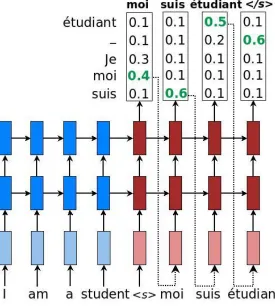
3.7.1 Greedy

As soon as the decoder gets the starting symbol < s > from the encoder, for each time step on

logit value is chosen. This is then passed in as input to the next time step. This process is continued

until the end of sentence marker < /s >is reached. The figure below shows greedy inference very

well.

Figure 3.2 Greedy decoding obtained from Luong et al. (9)

3.7.2 Beam Search

Beam Search uses breadth-first search to build its search tree but only keeps the top N (beam

size) nodes at each level in memory. The next level is then expanded from those N nodes. Its

3.8 Testing mechanism

3.8.1 BLEU scores

The Billingual Evaluation Understudy (BLEU) score Papineni et al. (2) is a common way to

find how well a machine translation system performed when there can be multiple good outputs.

Consider the following example: In French: Le chat est sur le tapis Reference English translation:

The cat is on the mat NMT English translation: There is a cat on the mat.

Both the English translations are equally good. Suppose we had the MT model predict the

translation to be The the the the the we know this is not a very good translation but we need to

measure exactly how bad this is. The BLEU score gives us this measure. It uses n-grams and finds

what fraction of the n-grams in the machine translation output also exist in the references. The

metric ranges from 0 to 1 and few translations attain a score of 1 unless they are identical to the

reference translation.

3.9 Random Search

For a long time, grid search (building a model for every configuration of hyperparameters and

evaluating each model) and manual search were the most widely used strategies for hyperparameter

optimization. In 2012, two researchers from the University of Montreal introduced random search

in their paper ”Random Search for Hyper-Parameter Optimization” (3). Random search is a very

simple concept – random combinations of the hyperparameters are chosen and trained. Random

search seemed to find the better models by effectively searching a larger, less promising configuration

space.

3.10 Successive Halving

Successive halving is an improvement over random search. The idea of successive halving is to

first try N hyperparameter settings for some fixed amount of time T. Then, we keep N/2 of the

to temporarily halt the training of a model, save the model and then proceed with the training.

The latter part can be problematic when using open source neural network models as it might be

difficult to stop and restart the training at any time with different configurations. Our adaptation

works around this issue by simply training them to completion and showing that the same results

can be obtained.

3.11 Hyperband

The paper for Hyperband can be refered from Li et al (15) Hyperband adopts both random

search and successive halving for hyperparameter optimization. It is a bandit-based strategy for

hyperparameter optimization that iteratively allocates resources to a set of random configurations.

Given a predefined budget B for one iteration, like time or total number of epochs, Hyperband

samples a fixed number of configurations uniformly at random and uses successive halving to discard

poorly performing configurations. The following steps explains the algorithm in more detail

1. Randomly sample a set of hyperparameter configurations

2. Evaluate the performances of all currently remaining configurations.

3. Throw out the bottom half of the worst performing configurations.

4. Repeat step 2 until only one configuration remains.

3.12 Proposed Algorithm

In our implementation of hyperparameter optimization we perform a slight modification in the

successive halving phase.

We allow each of the configurations to execute to completion before making a decision to discard

or keep that particular configuration. In addition, adaptive learning rates is implemented where

the learning rate is increased in specific increments after starting from a specific minimum. We

ended up checking for the learning rate after deciding on the other hyperparameters.The algorithm

Algorithm 1 Modified Successive Halving

input: previous configurations O, record of previously obtained BLEU scores B, number of configurations N, number of epochsE

output: The BLEU score for current configuration; the next configuration to consider C

while N != 1 do if O < N then

create random configurationC

TrainC

Record BLEU score binB O+ +;

else

for allconfigs C inO do

Find N/2 configurations with the highest BLEU scores.

N =N/2

Retrain the model with the different configurations.

Record the BLEU scores in B and repeat until only one configuration is left.

end for end if end while

As is evident, this algorithm is a combination of random search and successive halving. In

the first N configurations, the hyperparameters are randomly picked. In our implementation the

learning rate was picked in uniform random intervals from 0.0001 to 0.1. After the random search

was done, we resorted to successive halving by training N/2 number of configurations and doubling

the number of epochs. At this point, we also know a subset of the hyperparameters that work

better than the others so we can even reduce the range of different hyperparameters to choose

from. The main difference from regular successive halving is that we run each of the configurations

to completion instead of halting the model and changing the configurations and then continuing.

We found that this helps make the results more accurate although it takes more time to train to

completion.

Once the optimal set of hyperparameters are obtained, the learning rate was further configured

using the learning rate schedule. This helped us find a subset of values that would help us obtain

CHAPTER 4. RESULTS

4.1 System Configurations:

The training was done on a CentOS system that was running the NVIDIA GeForce GTX 1080

GPU. The CPU used is Intel Xeon CPU E5-2620 v3 with a 2.40GHz clock. It has 12 CPU cores

and a 64GB RAM.

4.2 Training Data:

The English-Vietnamese parallel corpus of TED talks (133K sentence pairs) provided by the

IWSLT Evaluation Campaign.

For the large scale training we used the German-English parallel corpus (4.5M sentence pairs)

provided by the WMT Evaluation Campaign.

4.3 Evaluation

Random search was first applied and each of the model configurations were trained for 6000

epochs. The results are shown in Table 4.1 and 4.2

It is clear to see that beam search and greedy inference modes performed better than the sample

inference. Using successive halving, we can choose the top 4 performing configurations and run

them for 12,000 epochs. The BLEU scores improved significantly. When beam search is used, the

beam width is always 10. The results are shown in Table 4.3

After narrowing down the four configurations from successive halving, it is clear which

con-figuration is the best for the given dataset. Keeping other hyperparameters the same, the luong

attention model seemed to outperform the bahdanau attention. In addition, for the given dataset,

the standard attention architecture seemed to perform better than the GNMT architecture. This

6000 epochs

Hyperparameters Config 1 Config 2 Config 3 Config 4 Learning rate 0.001392 0.03648 0.00993 0.01135

Optimizer sgd sgd sgd adam

Type of attention luong luong bahdanau luong Attention

Archi-tecture

standard standard standard gnmtV2

Inference mode sample sample greedy beam search; beam width 10

BLEU dev 0.0 0.2 5.3 5.6

BLEU test 0.0 0.4 1.4 1.4

Table 4.1 The different hyperparameter configurations obtained via random search

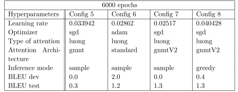
6000 epochs

Hyperparameters Config 5 Config 6 Config 7 Config 8 Learning rate 0.033942 0.02862 0.02517 0.040428

Optimizer sgd adam sgd sgd

Type of attention luong luong luong luong Attention

Archi-tecture

gnmt standard gnmtV2 gnmtV2

Inference mode sample sample sample greedy

BLEU dev 0.0 2.0 0.0 0.4

BLEU test 0.3 1.2 1.3 1.3

Table 4.2 The different hyperparameter configurations obtained via random search

adam optimizer, GNMT architecture, bahdanau attention adn beam search inference performed

way worse than the other configurations in table 4.3. So we discarded that set of hyperparameters.

We ran the given configuration for 24000 epochs. Although we only needed to train one of the

configurations, we trained the model with a a different inference mode. It was interesting to see

how beam search performed slightly better than greedy when the other configurations remained

the same. The encoders used for the Vietnamese-English translation was unidirectional. The State

of the art results mentioned below uses the bidirectional encoder.

We observe that beam search clearly helps the model perform better than greedy. The current

12000 epochs

Hyperparameters Config 1 Config 2 Config 3 Config 4 Learning rate 0.001392 0.03648 0.00993 0.01135

Optimizer sgd adam sgd sgd

Type of attention luong bahdanau luong bahdanau Attention

Archi-tecture

standard gnmtV2 gnmtV2 standard

Inference mode greedy beam search

beam search

greedy

BLEU dev 14.1 6.0 11.6 11.7

BLEU test 16.1 5.1 12.8 12.3

Table 4.3 The different hyperparameter configurations obtained via successive halving

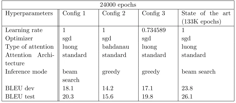
24000 epochs

Hyperparameters Config 1 Config 2 Config 3 State of the art (133K epochs) Learning rate 1 1 0.734589 1

Optimizer sgd sgd sgd sgd

Type of attention luong bahdanau luong luong Attention

Archi-tecture

standard standard standard standard

Inference mode beam search

greedy greedy beam search

BLEU dev 18.1 14.2 17.1 23.8 BLEU test 20.3 15.6 19.8 26.1

Table 4.4 The final hyperparameter configurations for the given model and dataset

fixed amount of active candidates at each time step. The greedy strategy only compares one

most-likely candidate. Thus the larger search space could help beam search make better judgements

about past word relationships. Some other observations we made are that – Adam optimizer

tends to give reasonable results for unfamiliar architectures but SGD with scheduled learning rate

tends to lead to better performance. Luong style works well with different settings. But from

other resources we find out that Bahdanau style attention often works better with bidirectionality

on the encoder side. For the Vietnameese-English translations, unidirectional encoders and the

standard architecture worked very well. However when we trained the German-English dataset,

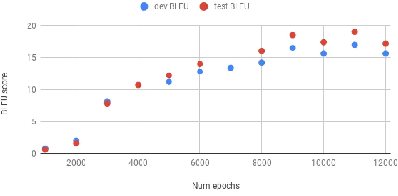
In the following figures, all the experiments are trained with the configuration:

• Number of epochs - 6000

• Optimizer - sgd

• Type of attention - Luong

• Encoder - uni-directional

• Inference mode - Beam search

Figure 4.1 The variation of the BLEU for every step in the training process

We see a near logarithmic increase in the BLEU scores. There is a high of 18.1 at around 11,000

epochs.

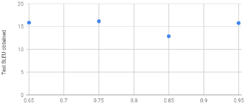
From the learning rate schedule, we can see that the BLEU score was at its best when the

learning rate was between 0.65 to 0.75. The next thing to try would be to create another schedule

and increase the learning rate with smaller increments to narrow down the prospects. Figures 4.3

Figure 4.2 The variation of the BLEU score obtained with respect to different learning rates. The congiguration used was

Figure 4.3 Vietnamese to English translations

For the German to English translations we found the optimal parameters to be

-• Optimizer - sgd

• Type of attention - normed bahdanau

• Attention architecture - gnmtV2

• Encoder - Gnmt

Figure 4.4 Vietnamese to English translations

We trained this configuration to 122,000 steps and got a dev BLEU score of 22.2 and a test

BLEU of 22.4. Fig 4.5 and 4.6 show some of the results obtained from these tests.

Figure 4.5 German to English translation at epoch 122000

CHAPTER 5. SUMMARY AND DISCUSSION

Machine Translation has seen significant progress over the last few years. In this work we showed

that a layered LSTM layer like in the sequence to sequence learning model and the GNMT model

work differently on different datasets. In addition, every hyperparameter affects the performance

of the model. When making any model, we have an idea about the top hyperparameters that

affect the model the most and in the case of NMT, the attention architecture, optimizers, attention

mechanism and the inference mode can significantly impact the results and performance of the

model.

We need to keep in mind that not all datasets work with the configurations shown in this report.

The report only covers the Vietnamese to English and the German to English translations. Given

a different dataset, it is difficult to pinpoint exactly what configuration would be the most optimal,

but we can narrow down the options by utilizing one of the hyperparameter optimization methods

described in this report.

Further work can be put into exploring other algorithms for finding the learning rate. This

report introduced adaptive learning rates but it would be interesting to explore search algorithms

for continuous variables to hone in on a good learning rate. In addition, more research can be put

REFERENCES

[1] Bengio Yoshua., Simard Patrice., Frasconi Paolo. (1994). Learning Long-Term Dependencies

with Gradient Descent is Difficult.IEEE Transactions on Neural Networks,

[2] Papineni Kishore., Roukos Salim., Ward Todd., Xhu Wei-Jing (2002) BLEU: a Method for

Au-tomatic Evaluation of Machine TranslationAssociation for Computational Linguistics (ACL)

[3] James Bergstra., Yoshua Bengio. (2012) Random Search for Hyper-Parameter Optimization.

Journal of Machine Learning Research 13 (2012) 281-305

[4] Srtvastava Nitish, Hinton Geoffery, Krizhevsky Alex, Sutskever Ilya, Salakhutdinov Ruslan.

(2014) Droupout: A Simple Way to Prevent Neural Networks from Overfitting. Journal of

Machine Learning Research 15 (2014)

[5] Sutskever Iiya., Vinyals Oriol., Le V. Quoc (2014). Sequence to Sequence Learning with Neural

Networks.NIPS 2014.

[6] Luong Minh-Tang., Pham Hieu., Manning D. Christopher. (2015) Effective Approaches to

Attention-based Neural Machine Translation. arXiv:1508.04025

[7] Yonghui Wu, Mike Schuster, Zhifeng Chen, Quoc V. Le, Mohammad Norouzi, Wolfgang

Macherey, Maxim Krikun, Yuan Cao, Qin Gao, Klaus Macherey, Jeff Klingner, Apurva Shah,

Melvin Johnson, Xiaobing Liu, ukasz Kaiser, Stephan Gouws, Yoshikiyo Kato, Taku Kudo,

Hideto Kazawa, Keith Stevens, George Kurian, Nishant Patil, Wei Wang, Cliff Young, Jason

Smith, Jason Riesa, Alex Rudnick, Oriol Vinyals, Greg Corrado, Macduff Hughes, Jeffrey Dean

(2016) Googles Neural Machine Translation System: Bridging the Gap between Human and

[8] Zhou, J., Cao, Y., Wang, X., Li, P., and Xu, W. (2016). Deep Recurrent Models with

Fast-Forward Connections for Neural Machine Translation.CoRR abs

[9] Minh-Thang Luong., Eugene Brevdo., Rui Zhao. (2017). Neural Machine Translation (seq2seq)

Tutorialhttps://github.com/tensorflow/nmt,

[10] Vaswani Ashish, Shazeer Noam, Parmar Niki, Uszkoreit Jakob, Jones Llion, Gomez N Aidan,

Kaiser Lukasz and Polosukhin Illia. Attention Is All You Need.arXiv:1706.03762v5,

[11] Peters E. Matthew., Neumann Mark., Iyyer Mohit., Gardner Matt., Clark Christopher.,

Lee Kenton., Zettlemoyer Luke. (2018) ELMo - Deep Contextualized Word Representations

NAACL,

[12] Devlin Jacob, Chang Ming-Wei, Lee Kenton and Toutanova Kristina. (2018) BERT:

Pre-training of Deep Bidirectional Transformers for Language Understanding.arXiv:1810.04805,

[13] Alammar Jay. (2018) The Illustrated Transformer.

http://jalammar.github.io/illustrated-transformer/

[14] spro. (2018) Practical PyTorch: Translation with a Sequence to Sequence Network and

At-tention.

https://github.com/spro/practical-pytorch/blob/master/seq2seq-translation/seq2seq-translation.ipynb

[15] Li Lisha, Jamieson Kevin, DeSalvo Giulia, Rostamizadeh Afshin, Talwalkar Ameet

(2018) Hyperband: A Novel Bandit-Based Approach to Hyperparameter Optimization

arXiv:1603.06560v4

[OpenNMT] OpenNMT tutorials http://opennmt.net/OpenNMT/training/models/

[LSTM- Colah’s blog] Understanding LSTM Networks – colah’s blog