Time-Dependent Real-Space Renormalization Group Method

(1)

Time-Dependent Real-Space Renormalization

Group Method

H. Raeisian Amiri

1,*

and F. Ebrahimi

2

1

Department of Physics, Tarbiat Modarres University, Tehran 14155-4838, Islamic Republic of Iran 2

Department of Physics, Shahid Beheshti University, Evin, Tehran 19839, Islamic Republic of Iran

Abstract

In this paper, using the tight-binding model, we extend the real-space

renormalization group method to time-dependent Hamiltonians. We drive the

time-dependent recursion relations for the renormalized tight-binding Hamiltonian

by decimating selective sites of lattice iteratively. The formalism is then used for

the calculation of the local density of electronic states for a one dimensional

quantum wire with time-dependent random potential. Specifically, we study the

electronic densities of states of a single and chains of quantum dots connected to

two noisy leads.

Keywords: Renormalization group; Time-dependent; Quantum dot

*

E-mail: hraeisian@ikiu.ac.ir

1. Introduction

Nowadays, nanostructures are commonly employed in electronic and optoelectronic devices [1,2] especially, devices based on one-dimensional (1D) systems have received considerable attentions [3]. Within the theoretical methods for studying 1D systems, the technique of the real space renormalization group, due to its simplicity, has been used extensively, both for ordered and disordered time-independent systems [4]. Many nanostructures, such as quantum dot, in connection to leads experience time dependent random potentials, either through their interactions with the environment or the inherent noise present in the system[5-7]. So, it is vital to determine their effects on the electronic properties of the nanostructures. In this paper, we extend the real-space renormalization group method (decimation method) to time dependent problems. Firstly, wederive the time-dependent recursion relations for the renormalized 1D

tight-binding (TB) Hamiltonian. Then, regarding reference [8], we extend the formalism to TB Hamiltonians with time-dependent random potentials. At the end, we apply the developed formalism to study the densities of electronic states of a single and chains of quantum dots in contact with two noisy leads.

2. Theory

(2)

hopping of the form

[

]

( ) ( ) ( )

( )

† †

1 , 1 1 1 1 1 †

, 1 1 1 1 1

( ) ( ) ( ) ( )

,

, ( ) (

n n n n

n

o

n n n n

n

o

n n n n

H t V t a t a t

dt T t t a t a t

T t t a t a t

ν − − + + = + + ⎡ + ⎣ ⎤⎦

∑

∑∫

) (1)

where is the on-site static potential and Vn(t) and

Tn,n±1(t,t1), are respectively, time-dependent on-site

potential and nearest neighbor hoppings.

n

v

The time-dependent Green's function associated with the above Hamiltonian satisfies the following time evolution equation

( )

[

]

( )

(

)

(

)

, ,

1 , 1 1 1,

, 1 1 1, 1 ,

, ( ) ( , )

, ,

m n m m m n

o

m m m n

o

m m m n n m

i G t t V t G t t

t

dt T t t G t t

T t t G t t t t

ν δ δ + + − − ∂ _′ ₋ ₊ _′ ₊ ∂ ⎡ ′ + ⎣ ⎤ ′_⎦= − ′

∫

h (2)

Defining the on-site Green's function, g t tn0( , )′ , as the inverse of the operator [i V tn( ) v

t

∂ ₋ ₋

∂

h n]

,

, we can rewrite Equation (2) as

( )

(

)

(

)

(

)

(

)

, ,

1 2 1 , 1 1 2 1, 2 , 1 1 2 1, 2

, ,

o

m n m m n

o o

m m m m n

o

m m m n

G t t g t t

dt dt g t t T t t G t t

T t t G t t

δ + + − − ′ = ′ − ⎡ ′ + ⎣ ⎤ ′ ⎦

∫ ∫

(3)

An iterative procedure can now be used to solve for by eliminating the equations containing odd sites and re-numbering the sites, at each iteration step. After each iteration the resulting equation has a structure similar to Equation (3) but with renormalized on-site Green's function and hopping terms. After jth

decimation the renormalized quantities, are given by the recursion relations

00( , )

G t t′

( 1)

( 1) ( 1),

( ) , 2

( 1) 1 2 , 2 1

( 1) ( 1)

1 2 2

2 2 2

( , )

( , ) ( , )

j

j j m j

j m m j m m j j m m

T t t

dt dt T t t

g t t T t t

− − − + − + − − + + + ′ = − ′

∫ ∫

(4)

( 1)

( 1) ( 1)

( ) , 2

( 1) 1 2 , 2 1

( 1) ( 1)

1 2 2

2 2 , 2

( , )

( , ) ( , )

j

j j j

j m m

j j

m m m

T t t

dt dt T t t

g t t T t t

− − − + − − − − − − − ′ = − ′

∫ ∫

(5)

and ( ) ( ) _{( )} 1 1 ( ) ( , ) ( , ) ( , ) ( ) j

m m m

j _j

m n

m

i V t g t t

t

dt t t g t t t t

ν ,m δ δ ∂ ⎡ ₋ ₊ ⎤ _′ ⎢_∂ ⎥ ⎣ ⎦ ′ ′ −

∫

∑

= h − (6)

where ( )j ( , )

m t t′

∑

is given by

( 1) ( 1) ( 1)

( ) ( 1)

( 1) ( 1) ( 1)

1 1 2 2

, 2 2 2 ,

1 2

( 1) ( 1) ( 1)

1 1 2 2

, 2 2 2 ,

( , ) ( , )

( , ) ( , ) ( , )

j j j

j j

m m

j j j

m m m m m

j j j

m m m m m

t t t t

T t t g t t T t t

dt dt

T t t g t t T t t

− − − − − − − − − − + + + − − − − − − ′ = − ′ ⎡ ′ +⎤ ⎢ ⎥ − _⎢ _⎥ ′ ⎢ ⎥ ⎣ ⎦

∑

∫ ∫

(7)

In the above equations ( )_, ₂j( , ),

j m m

T ₊ t t′ 1

( )

2j ( , )

j m

g ₊ − t t′

and ( )j ( , )

m t t′

∑

are, respectively, the renormalized

hopping term, on-site Greens

,

function and the self-energy after the jth decimation.

To use the above recursion relations, the equation for

( ) ( )( , )

j m

g t t′ at each iteration step should be solved. This equation is an integro-differential equation which can be solved iteratively. It should be mentioned that all the Green's function are retarded. The above formalism can also be used for random time-dependent potentials concerning references [8-10]; i.e. at each step of decimation the dependence of the renormalized quantities on the readom potentials associated with decimated sites are averaged [11,12].

The quantity of fundamental importance for applying the dependent RG method to random time-dependent potentials is the averaged on-site Green's function which we denote it by (( ))( , )

j m

g t t′ . The averaged on-site Green's function should be determined at each step of the iteration by solving the averaged form of Equation (6). To obtain the equation for averaged on-sit Green's function, we rewrite Equation (6) as

( ) ( ) ( )

( ) ( )

1 2 1 1 2 2

( , ) ( , ) ( , ) ( , ) ( , ) j o m m j o o

m m m

g t t g t t

dt dt g t t t t g t t

′ = ′ +

′ +

(3)

( )

( ) ( )

1 2 3 4 1 1 2 2 3

( ) ( ) 3 4 4 ( )

( ) ( )

1 2 1 1 2 2 3

( ) _{( )} 2 1 2 2

( , ) ( , ) ( , ) ( , ) ( , ) ... ... ( , ) ( , ) ( , )... ( , ) ( , ) . j o o

m m m

j o

m m

j

o o

n m _m m

j _o

n n m n

m

dt dt dt dt g t t t t g t t

t t g t t

dt dt g t t t t g t t

t ₋ t g t t

′ + + ′ + ..

∑

∫ ∫ ∫ ∫

∑

∫

∑

(8)

Denoting the averaging over the random potentials by ... , we have to determine the average of products of g((0) 'm)s and

( ) 'j

m s

∑

. But, since they are retarded all the time variables used in the integrals are time ordered, so averaging process for various terms in the product is carried out at different times, therefore, we have

( ) ( )

1 1 2 2 1 2 2

( ) ( )

1 1 2

( ) _{( )}

2 1 2 2

( , ) ( , )... ( , ) ( , )

( , ) ( , ) ...

( , ) ( , )

j j

o

m _m _m n n

j o

m m

j _o

n n m n

m

g t t t t t t g t t

g t t t t

t t g t t

−

′ o

m n =

′

∑

(9)

Thus, the equation that determines the averaged on-site Green's function is

( ) ( ) ( )

( ) ( )

1 2 1 1 2 2

( )

( ) ( )

1 2 1 1 2 2 3

( ) ( )

2 1 2 2

( , ) ( , ) ( , ) ( , ) ( , ) ... ... ( , ) ( , ) ( , ) ... ( , ) ( , ) ... j o m m j o o

m m m

j

o o

n m _m m

j o

n n m n

m

g t t g t t

dt dt g t t t t g t t

t ₋ t g t t

′ = ′ + ′ + + ′ +

∑

∫ ∫

∑

∫

∑

(10)

Using Equations (4) and (5) the averaged value of renormalized hoppings can be calculated once the averaged on-site Green's function is determined.

3. Applications and Results

In this section the formalism of time-dependent renormalization group will be used to study the effects of noisy leads on the densities of states of a single and chains of quantum dots. For simplicity, we consider a quantum wire in TB approximation where all the sites, except a finite number of them, are driven by time-dependent random potential, . For simplicity, we assume that the hoppings between the leads and the quantum dots are equal to the hoppings within the leads and they are independent of time. The Hamiltonian of the dots and the leads takes the simple from

( ) m V t

[

]

† † † 1 1

( ) _m( ) _m _m

m

m m m m

m

H t V t a

T a a a a

ν

∞

=−∞

− +

= + a

⎡ ⎤

+ _⎣ + _⎦

∑

(11)

where ' are the on-site static potentials and

m

v s V_m( )t s′

are zero on the dots. We, also, choose to be Gaussian noise with

( ) m

V t

( ) ( ) ( )

m n m n

V t V t′ =F δ t − ′t δ _m (12)

where F sm′ are parameters defining the distribution and

the brackets ... indicate statistical averages and n,m

corresponding to the sites in the leads.

The Gaussian noise is completely defined by its generating function

exp ( ) ( )

1

exp ( ) ( ) ( ) ( )

2

n n

n

n m n m

i dt t V t

dt dt t t V t V t

∞ −∞ ∞ ∞ −∞ −∞ ⎛ ⎞ Φ = ⎜ ⎟ ⎜ ⎟ ⎝ ⎠ ⎛ ⎞ ′ ′ ′

− Φ Φ

⎜ ⎟ ⎜ ⎟ ⎝ ⎠

∑ ∫

∫ ∫

(13)

where Φ_n( )t′_s are test functions. Functionally differentiating the generating function with respect to

( )

m t s′

Φ r-times and setting to zero after differentiation, we obtain the statistical average of

( )

m t s′

Φ

1( )...1 ( )

m mr r

V t V t . For the above Hamiltonian, the on-site retarded Green's function has the form

( )

1 1

( , )

( ) exp ( )

exp ( ) , 0, 1, 2,...

o m m t m t

g t t

i i

t t t t

i

dt V t m

θ ν ′ ′ = − ⎛ ⎞ ′ ′ − − _⎜ − _⎟ ⎝ ⎠ ⎛− ⎞ = ± ± ⎜ ⎟ ⎜ ⎟ ⎝

∫

⎠ h h h (14)

and its statistical average is given by

( )

1 1

( , )

( ) exp ( )

exp ( ) , 0, 1, 2,...

o m m t m t

g t t

i i

t t t t

i

dt V t m

θ ν ′ ′ = − ⎛ ⎞ ′ ′ − − _⎜ − _⎟ ⎝ ⎠ ⎛− ⎞ = ± ± ⎜ ⎟ ⎜ ⎟ ⎝

∫

⎠ h h h (15)

(4)

Green's function is given by

( )_{( , )}

( ) exp ( )

1 exp

2 o

m

g t t

i i

t t t t

F t t

θ ν

′ =

−

⎛ ⎞

′ ′

− − _⎜ − _⎟

⎝ ⎠

−

⎛ ₋ _′⎞

⎜ ⎟

⎝ ⎠

h h (16)

Considering that

( , ) ( )

o n

T t t′ =Tδ t− ′t (17)

for the Hamiltonian given by Equation (11), we can use the recursion relations (4), and (5), and Equations (7), and (8), after averaging the decimated sites, to obtain the renormalized hoppings and on-site Green's function. For Gaussian noise the averaged retarded on-site Green's function is a function of time-difference. Thus, we can solve Equation (10) using Fourier Transform (FT) with respect to time variable. This reduces the integral Equation (10) to algebric eqiatopn

( ) ( ) ( )

( ) ( )

( )

( ) ( )

( ) _{( )}

( ) ( )

( ) ( ) ( )

... ( ) ( ) ( ) ...

( ) ( ) ...

j o

m m

j

o o

m _m m

j

o o

m m m

j _o

m m

g E g E

g E E g E

E g E

= +

+

∑

(18)

or

( ) ( )

( )

( ) ( )

( ) ( ) ( )

j o

m m

j

o j

m m m

g E g E

g E E g

= +

∑

E

(19)

which has the form of Dyson equation. Equation (19) can be solved for ( )

( )

j m

g E , which gives us

( ) ( )

( ) (0)

( ) ( )

1 ( ) (

o m j

m _j

m m

g E

)

g E E

=

−

∑

(20)

We can, also, FT the recursion relations, Equations (4) and (5), for renormalized hoppings and Equation (7) for . This reduces Equations (4), (5) and (7), respectively, to

( )

( , ) j

m t t′

∑

( )

( 1) ( 1) ( 1) ( )

( ) , 2

( 1) ( 1) ( 1)

, 2 2 2 , 2

( )

( ) ( ) ( )

j

j j j j

j m m

j j j

m m m m m

T E

T − E g − E T −

+

− − −

+ + + +

=

− E

E

(21)

( )

( 1) ( 1) ( 1) ( )

( ) , 2

( 1) ( 1) ( 1)

, 2 2 2 , 2

( )

( ) ( ) ( )

j

j j j j

j m m

j j j

m m m m m

T E

T − E g − E T −

−

− − −

− + − −

=

− (22)

and

( 1) ( 1) ( 1) ( )

( )

( 1) ( 1) ( 1)

, 2 2 2 , 2

( 1) ( 1) ( 1)

, 2 2 2 , 2

( )

( ) ( ) ( )

j j j j

j

m

j j j

m m m m m

j j j

m m m m m

E

T E g E T E

T E g E T

− − −

+ + + +

− − −

− − − −

=

− −

∑

(23)

Equations (20)-(23) including Equation (16) constitute the renormalized recursion relation for a system driven by a Gaussian noise.

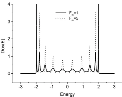
We now consider the effects of noisy leads with Gaussian distributions on the local densities of states of a single and finite chain of quantum dots. For a single quantum dots, we assume that the dot is located at the site m= 0 and the Gaussian noise acts on all the sites of left and right leads with a same strength. Figure 1 represents the local densities of states for three different values of F sm′ . Figures 2 and 3 depict, respectively, the

local densities of states of a quantum dot located at site

m = 0 within the chains with 11 and 19 quantum dots for two different values of F s_m′ . We observe from Figure 1 that in the case of a single quantum dot the noise in the leads causes the states of the dot to become more localized around zero energy state. The effect of localization also appears in the chains. For weak noise it manifests itself as an oscillation in the local densities of states. As the strength of noise increases, the states of quantum dot become more localized around definite

(5)

Figure 2. The local densities of states of a quantum dot located at m=0 within the chain of eleven quantum dots, connected to noisy leads for two different values of F_m′s in unit of hopping integral.

Figure 3. The local densities of states of a quantum dot located at m=0 within the chain of nineteen quantum dots, connected to noisy leads for two different values of F_m′s in unit of hopping integral.

energy values. These behaviors of local densities of states are reminiscence of a leaky double barriers; i.e.

each noisy lead acts as a leaky barrier for electrons in the quantum dot or in the chains.

In conclusion, in this paper we have presented the time-dependent real space renormalization group method which is a versatile numerical technique for studying the effects of various time-dependent random potentials with any kinds of distributions [13,14]. We have then used the proposed method for studying the effects of noisy leads with Gaussian distribution on the densities of states of single and chains of quantum dots. The method can, also, be extended to include, concurrently, static as well as time-dependent random potentials and hopping integrals.

Acknowledgement

We would like to acknowledge the assistance of Dr. E. Faizabadi and M. Bagheri.

Rrferences

1. Harrison P. Quantum Wells, Wires and Dots. John Wile and Sons (2000).

2. Datta S. Electronic Transport in Mesoscopic Systems. Cambridge University Press (1995).

3. Goncalves da Silva C.E.T. and Schlottmann P. Solid State Communication, 41: 11,819 (1982).

4. Koiller B., Robbins M.O., Davidovich M.A., and Concalves da Silva C.E.T. Ibid., 45: 11,955 (1983). 5. Buttiker M. J. Math. Phys., 37(10): 4793 (1996).

6. Kattine J.A., Berry M.J., and Westavelt R.M. Phys. Rev., B57: 1693 (1998).

7. Cuniberti G., Sassetti M., and Kramei B. Ibid., B57: 1515 (1998).

8. Liu Y. Ibid., B33(2): 1010 (1986).

9. Ostlund S. and Pandit R. Ibid., B29(3): 1394 (1984). 10. Jaime Ramirez Ibanez R. and Silva C.E.T.G. Ibid.,

B31(4): 2464 (1985).

11. Robbins M.O. and Koiller B. Ibid., B27(12): 7703 (1983). 12. Bhattacharjce A.K. and Goncalves da Silva C.E.T. Solid

State Communication, 45: 8,673 (1983).

13. Suqing D. and Zhao X.-G. Phys. Rev., B61(8): 5442 (2000).