Please cite this article asF Yaghmaee, H Reza Koohi,Dynamic Obstacle Avoidance by Distributed Algorithm based on Reinforcement Learning, International Journal of Engineering (IJE), TRANSACTIONS B: Applications Vol. 28, No. 2, (February 2015) 198-205
International Journal of Engineering
J o u r n a l H o m e p a g e : w w w . i j e . i r
Dynamic Obstacle Avoidance by Distributed Algorithm based on Reinforcement
Learning
F Yaghmaee*, H Reza Koohi
Electrical and Computer Engineering Department, Semnan University, Semnan, Iran
P A P E R I N F O
Paper history: Received 02 July 2014
Received in revised form 07 October 2014 Accepted 13 November 2014
Keywords:
Reinforcement Learning, Sensor Network Dynamic Obstacle Avoidance
Robot Navigation.
A B S T R A C T
In this paper, we focus on the application of reinforcement learning to obstacle avoidance in dynamic environments in wireless sensor networks. A distributed algorithm based on reinforcement learning is developed for sensor networks to guide mobile robot through the dynamic obstacles. The sensor network models the danger of the area under coverage as obstacles, and has the property of adoption of itself against possible changes. The proposed protocol can integrate the reward computation of the sensors with information of the intended place of robot so that it guides the robot step by step through the sensor network by choosing the safest path in dangerous zones. Simulation results show that the mobile robot can get to the target point without colliding with any obstacle after a period of learning. Also, we discussed about time propagation between obstacle, goal, and mobile robot information. Experimental results show that our proposed method has the ability of fast adoption in real applications in wireless sensor networks.
doi: 10.5829/idosi.ije.2015.28.02b.05
1. INTRODUCTION1
We use reinforcement learning under so-called “dynamic reinforcement” in wireless sensor network to guide mobile robot through the dynamic obstacles. Reinforcement learning dates to early days of cybernetics and work in statistics, psychology, neuroscience, and computer science. In the past 20 years, it has attracted rapidly increasing interest in machine learning and artificial intelligence communities [1]. In reinforcement learning, each agent repeatedly interacts with an unknown environment, receives a reward or punishment, and updates the probabilities of its next action based on its own previous actions and received values.
Autonomous mobile robots have a wide range of application, such as in hospitals, houses, industries, space exploration, etc. Generally, obstacle avoidance is the main aspect of mobile robot. The purpose of obstacle avoidance is to enabling mobile robots to get to the target point without colliding with any obstacle in
1*Corresponding Author’s Email:[email protected] (Farzin Yaghmaee)
unknown or dynamic environments. The conventional control technique is model based called planning architecture and artificial potential fields and cell decomposition belong to this type of controller [2]. However, this model needs a long time to execute an action and also is limited to known environments. Moreover, weak robustness is a problem in this model. Behavior-based architecture [3] is different from planning architecture which has many advantages, such as better robustness and quickness. In order to adopt this architecture to complex and dynamic environments without the further intervention, learning ability should be adopted to improve the autonomy of mobile robots. Reinforcement learning [4-8] is used widely and can be applied to the behavior-based architecture. In [9] discuss about the reinforcement learning in complex multi-agent learning problem.
In this paper, distributed algorithms based on reinforcement learning is developed for sensor network to guide mobile robot through the dynamic obstacles like burning area in real world. A series of operating sensors which have been networked together can follow the movements of robot in dangerous environment and direct it to desired point. By assuming dangerous places
as obstacles, we calculate the reward or punishment based on obstacles that will be in tune with current system's status. Base on these values, safest path to goal will produce which means it evades the least number of traces of danger.
The rest of paper is as follows: in section 2 we briefly explain important ideas in reinforcement algorithm. In section 3, proposed method is fully described and simulation results are presented in section 4. Finally, conclusion comes in section 5.
2. REINFORCEMENT LEARNING MODEL
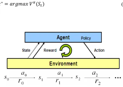
Reinforcement learning is used to learn the internal structure of the behaviors by mapping the perceived states to control actions while maximizing the accumulated reinforcement reward. In reinforcement learning process, the agent perceives the state of the environment and receives an input that describes the state. Then, the agent chooses an action from the action set to execute immediately and agent possibly moves to a new state. After that, the agent receives an evaluation feedback called reinforcement as well as perceives the new state. The purpose of the learning system is to find a control policy that maximizes the expected amount of reward during the whole learning period. The value function can be described as Equation (1):
( )≡ + . + . +⋯ (1)
where, is the reward received in transition from state to state and g (0<g<1) is the discount factor.
( ) is the discounted amount reward received by the learning system since time t . It depends on the sequence of chosen action which is determined by the strategy of control. The system has to find a control strategy that maximizes ( )for each state. The model of RL(Reinforcement Learning) is shown in Figure 1.
Once the target function in Equation (1) is determined, the optimal behavior policy can be expressed as Equation (2):
∗= ( ) (2)
Figure 1. Model of Reinforcement Learning
Reinforcement learning obtains its optimal policy based on its feedback. Unlike supervised learning, RL needs no training sequences. In [1, 4, 5] more discussion about Q-learning based on Markov Decision Process is presented.
3. PROPOSED DISTRIBUTED ALGORITHM FOR SENSOR NETWORK
Sensors collect information from different areas. They can store information locally or route them to a base station for further analysis and use. Sensors can also use communicative facilities to integrate their sensed values with the rest of the sensor landscape. We will discuss a method to distribute the information about the environment redundantly across the entire network. Robot can use this information as they traverse the network. It’s also guided across the network along a safe path, away from the type of danger that can be detected by the sensors.
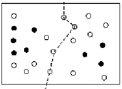
The dangerous areas in the sensor network will be defined as obstacles. Danger may include overheating, fire, hazardous gasses, thick fume, etc. It is supposed that each sensor can sense the presence or absence of such types of danger. An iterative danger configuration protocol running across all the nodes of the network creates the danger map. We do not envision that the network will create accurate geometric map, distributed across all the nodes. Instead, we wish to provide some information about how far from danger each node is in network. If the sensors are uniformly distributed, the smallest number of communication hops to a sensor that triggers "yes" to danger is a measure of the distance to danger. The idea is to find a path for a robot that avoids the dangerous areas. We suppose that the user ask the network regularly for where to go next. The nodes within broadcasting range from the user supply to the next best state.
Figure 2. A typical example of navigation guiding task.
Algorithm 1 shows the reward computation protocol. The reward is computed as each sensor whose triggers danger diffuses some information to its neighbors in a message that includes its source node id, the reward value, and the number of hops from the source of the message to the current node. When a node receives multiple messages from the same source node, it keeps only the message with the smallest number of hops. The message with the least hops is kept because that message is likely to travel along the shortest path. The current node will compute the new reward value from this source node. Then, the node broadcasts a message with its own reward value and number of hops to its neighbors.
After this configuration procedure, nodes may have several rewards from multiple resources; to compute its current danger level information each node adds all the rewards.
Algorithm 1: The Reward Computation Protocol.
1 for all sensors Si in the network do
2 puni= 0, hopsj= ∞ for any danger j
3 if sensed-value = danger then 4 hopsi = 0, puni = Infinity 5 Broadcast message (i, hops = 0) 6 if receive (j, hops) then 7 if hopsj >hops+1 then
8 hopsj =hops+1
9 Broadcast message (j;hopsj) 10 for all received j do
11 Compute the punishmentpunjof j using 1 2
j
j hops
pun =
12 Compute the reward & punish at Si using all
j
pun , puni =
i
pun + punj
, rewi=1 puni
It is to be noted that the reward protocol provides distributed repositoryof information about the area covered by the sensor network. It can be applied in an initialization phase, continuously or intermittently. The sensor network can self-organize adaptively to the current landscape. It updates its distributed information content by running the reward computation protocol regularly. In this way, the network can adapt to sensor
failure and to dynamic danger sources that can move across the network.
The reward value stored at each node can be used to guide robot equipped with a sensor that can establish an online interaction with the network. The safest path to the goal can be computed by using algorithm 2. The goal node initiates a dynamic programming computation of this path using broadcasting.
Algorithm 2: The safest path to goal computation protocol.
1 Let G be a goal sensor
2 G broadcasts msg= (Gid,myid(G), hops=0, reward= gv) //gv is a great value
3 for all sensors do
4 Initially hops = g ¥ and rg= 0
5 if receive (g, k, hops,reward) then
6 Compute the reward integration from the goal to here 7 if rg<reward+rewi then
8 rg=reward+rewi
9 hopsg=hops+1
10 prior k
g=
11 Broadcast (Gid, myid(Si),hops ,g rg)
The goal node broadcasts a message with the danger degree of the path, which is zero for the goal, you can find it by great value of goal node reward. When a sensor node receives a message, it adds its own reward value to the reward value provided in the message, and broadcasts a message updated with this new reward to its neighbors. If a node receives multiple messages, it selects the message with the greatest reward (corresponding to the least danger) and remembers the sender of the message.
Algorithm 3: The navigation guiding protocol.
1 if
i
S is a user sensor then 2 while Not at the goal G do 3 Broadcast inquiry message (Gid)
4 for all received messages m = (Gid,myid(Sk), hops, reward, prior) do
5 Choose the message m with maximal reward then minimal hops.
6 Let myid(Sk) be the id for the sender of this message
7 Move toward myid(Sk) and prior.
8 if
i
S is an information sensor then 9 if receive (Gid) inquiry message then
10 Reply with (Gid,myid(Si),hopsg,rg,priorg)
i
A robot in the sensor network can rely on the information computed using Algorithms 1 and 2 to get continuous feedback from the network on how to traverse the area. Algorithm 3 shows the navigation guiding protocol. The robot asks the network for where to go next. The neighboring nodes reply with their current values. The robot's sensor chooses the best possibility from the returned values. Note that this algorithm requires the integrated reward value computed by Algorithms 1 and 2 in order to avoid getting stuck in local minima.
3. 1. Some Notes for Implementation Our navigation algorithm has an implicit assumption that the communication paths in the network are bi-directional. Since based on reinforcement learning structure the safest path is computed backward from the goal, messages have to able to flow in the opposite direction to lead the user to the goal. However, all attachment is not always manipulated as bi-directional in sensor network. In [10, 11] discussed about the distribution of symmetric and asymmetric links in sensor network. As an additional protocol run by each node can perform neighbor profiling to find all stable one-hop neighbors bi-directionally; these neighbors should be reachable to and from the node with high probability. A side effect of neighbor profiling is the removal of many of the transient links that are active for a very short time.
Algorithms 1 and 2 ask each sensor upon receiving a message to broadcast with fewer hops to the dangerous area or with greater reward integration to the goal. Many of the broadcasts may not be necessary since only the message with the least hops to the danger node location or the maximal reward integration to the goal is useful. To reduce the message broadcasts, we let each sensor wait for some time before it broadcasts. The waiting time for sensor Si is proportional to hop in Algorithm 1 and the value rewi in Algorithm 2. By this way, only the messages that carry the optimal value will be broadcasted and those carrying the non-optimal value will be suppressed. It can prove that the number of message broadcasts for each sensor is 1 in each algorithm using this technique [12].
3. 2. Accuracy of Protocol Our protocols can correctly determine the safest path to the goal without getting stuck in the local minima.
Theorem 1: Algorithm 3 will always give the robot sensor a path to the goal.
Proof: In Algorithm 2, the prior link of a node points to a node that has reward value more than that of the current node. So, for each node other than the goal, there must be a neighboring node that has a greater reward value. This proves that there are no local minima in the network.
The robot's sensor can always find a node among its neighbors that leads to a greater reward value. If the process continues, the node will end up with the goal that has the greatest reward value. Therefore, Algorithm 3 can always give the mobile robot sensor a path to the goal.
3. 3. Communication Capabilities Two natural questions arise about the protocols we described previously:
· How much time does it take to propagate the obstacle and goal information?
· Is the network capable of transmitting all the information?
In this section, we answer the two questions in the context of our current implementation.
We assume that each node has fixed transmission range and nodes in a node's neighborhood (say k nodes) should be silent to avoid contention when that node broadcasts. For the obstacle information propagation, assume the number of the concerned obstacles is O; i.e., on average, each node has to process the information of
O obstacles. Let the transmission rate for each node be b s
packets . Then, time for obstacle information propagating to a node is okl b where l=min
(
L,lo)
, L is the distance for the reward value to become maximum, andl
o is the distance between the node and the obstacle, both in number of hops.The formula is for the case when we add waiting time for each broadcast; i.e., each node only broadcasts obstacle information propagation once. In this case, each node needs to wait for k btime before broadcasting the best value. This waiting time allows enough time for each of the node's neighbors to broadcast the packet if they hold the same value as this node, so that they do not collide. For the case without explicit waiting time scheme, the MAC protocol enforces this delay to make sure all the packets go through smoothly. On the other hand, suppose we do not have the waiting time scheme, each node may broadcast multiple times because the least number of hops is unlikely to be obtained by the first received message so that the node needs to broadcast several packets before the best value is propagated. In this case, we must multiply the propagation time by another parameter m, which is the average messages broadcast for each node. Similarly, we can evaluate the propagation time for the goal information.
hops away. When the obstacles are static, and we do not care about the time, the network is capable of transmitting this amount of bits. If we have some constraints on the time, say, we have moving obstacles and the location of an obstacle must be known to the network within a distance resolution d, the network may not be able to carry all the information. Suppose the maximal speed of the obstacle is v. In the worst case, an obstacle generates v d packets per time unit, so each node needs to process ov d packets, which should be less thanb k, i.e., ovd<b k. If we do not have the waiting time, we expect more packets be generated and the precision about the mobile agent represented by the network will be low.
Suppose a flame of fire is moving at a speed of 1 s
m , the maximal transmission rate for a node is 40 s
packets , the number of concerned obstacles is 1, and
the number of the concerned neighbors of a node is 8. The network can sustain updates at a resolution of 0.2 meters. If we have the same network, but the mobile agent is a vehicle moving at a speed of 30miles h, the vehicle updates can happen every 2.7 meters.
4. IMPLEMENTATION
Visual-Sense [13] from Ptolemy II simulation software package was used for simulation.
4. 1. CORRECTNESS VALIDATION Algorithms 1, 2, and 3 were simulated by using Visual-Sense. In simulation, we asked both the goals and the obstacles to generate the reward or punishment value and propagate it to the entire network periodically. This demonstrates that the goals and the obstacles can be added to the network at any time.
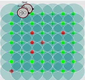
The goal is represented with a composite-wireless-actor. As shown in Fig. 3, the nodes in the network that can sense the danger (obstacle) are represented with components that have two concentric circles where internal green circle represents node and external blue circle represent transmission range. The robot that routes in the network is represented with another component.
A grid containing 7*7 nodes was used to simulate experimenting the performance and accuracy of protocols. We assume that sensors deployed on a building previously so these nodes were deployed symmetrically grid and all neighbors are within communication range. With this assumption, energy of the sensors can supply from the building energy source, but due to possibility of fire, it is better that sensors equipped with backup battery. The application is run by iterating a request for the next step by the user, a response by the network, and a move to the direction of
the network response. To implement this last part, we assume that the nodes know their location and it can be transmitted to the moving user. This can be done by augmenting nodes with a GPS location, or via triangulation. Since we have not done this augmentation of the hardware yet, we simulate location knowledge by placing the nodes in a grid pattern and supplying coordinates. The reward and goal-path computations are run by the network continuously, so it updates distributed information content, and the network can adapt to sensor failure and to dynamic danger sources which can move across the network.
When an obstacle or goal broadcasts, the receiving network node checks its list of known goals, and replaces the old data with the new broadcast if the new broadcast has a lower hop count. When a node receives a broadcast, it degrades the value of the broadcast based either on a linear function on the number of hops for goals or by the squared number of hops for obstacles. If the new value is not below a cutoff threshold, the packet is transmitted to its neighbors. When a user requests reward estimates, all nodes can hear it respond. The user chooses the node with the largest reward value (that is greater than the value of the current node). The user moves toward this node.
Figure 3: Simulation with 7*7 sensor nodes in a network by
means of Visual-Sense
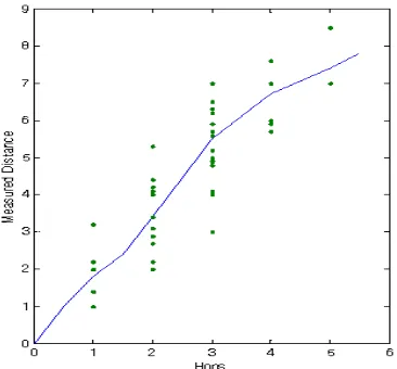
Figure 4: Results after the completion of simulation: Green
Figure 5. The comparison between the measured real distance and the hops counted using the presented algorithm
This Simulation proved that a user with a sensor node actually went around the obstacles and got to the goal, via the correct path. We observed that the network adapted to introducing of a new obstacle nodes quickly and robustly.
When a new obstacle is inserted in the network, the obstacle starts broadcasting its danger information which affects the information held by each node. At this point, Algorithms 1 and 2 cause the local information to change. We call the total time for the network to identify the new distances from danger and to the goal for each node the “time for the network to stabilize”. In other words, the time for the network to stabilize is the information propagation time in the network, which depends on the maximal hops from the goals or the obstacles to any node in the network. When an obstacle is added to the system online, it takes an identical amount of time to diffuse the information to the whole network.
Figure 5 shows the comparison between the measured real distance and the hops counted using our algorithm. The data was collected in our 7×7 grid network. We can see that the measured real distance is approximately linear in the number of hops.
4. 2. Some Notes on Hardware Implementation
Several interesting aspects of these experiments can be observed. The time for network stabilization (that is, the time for all the nodes to get the shortest distance to the danger source and the time for all the nodes to get the safest path to the goal) may take much longer than we expected. In our algorithms, we made two typical assumptions: (1) a node broadcasts the message received immediately and (2) each node gets the packet traveling through the shortest path. We observed that on the hardware test none of these assumptions was held. The network stabilization takes a long time because of
network congestion and transitory link status. Often, nodes seemingly out of range hear each other for brief moments of time. It seems that the following items are within the bounds of hardware implementation:
· Data loss: Data lose is not rare in sensor network. This is due to network congestion, transmission interference, and garbled messages.
· Asymmetric connection: It is observed that the transmission range in one direction may be quite different from that in the opposite direction. Thus, the assumption that if a node receives a packet from another node, it can send back a packet is too idealistic. In routing algorithm design, the existence of a route that can carry a packet from the source to a node does not guarantee a reverse route from that node to the source.
· Congestion: Network congestion is very likely when the message rate is high. This is aggravated when the nodes in proximity of each other try to send packets at the same time. For a sensor network, because of its small memory and simplified protocol stack, congestion is a big problem.
· Other unpredictable network conditions: In our sensor network nodes that should be several hops away from each other occasionally come in direct communication range. We expect many transitory links (on and off) in an unstable network due to the impact of unpredictable conditions.
5. CONCLUSION
We used reinforcement learning in sensor networks for better cooperation and adoption in dynamic environments. We have dealt with sensor networks for guiding the robot across the area of network on the safest path. Safety is measured as the distance between danger and detecting sensors.
In this paper, protocols based on reinforcement learning are suggested and have implemented on a distributed repository of information which can be retrieved efficiently whenever is needed. We have simulated these protocols on a 7×7 network of sensor nodes by using the Visual-Sense software from Ptolemy II package.
The contribution of our experimental evaluations is the time delay which is needed to network adapts itself to new situation such as detecting a moving object, detecting a new obstacle, adding a new sensor in the network, and removing a sensor from the network.
6. REFERENCES
Signal Processing, PacRim, Pacific Rim Conference on, IEEE., (2009), 319-324.
2. Chasparis, G.C. and Shamma, J.S., "Distributed dynamic reinforcement of efficient outcomes in multiagent coordination and network formation", Dynamic Games and Applications, Vol. 2, No. 1, (2012), 18-50.
3. Brooks, R.A., "A robust layered control system for a mobile robot", IEEE Journal ofRobotics and Automation, Vol. 2, No. 1, (1986), 14-23.
4. Gosavi, A., "A tutorial for reinforcement learning", Department of Engineering Management and Systems Engineering, (2011). 5. Busoniu, L., Babuska, R. and De Schutter, B., "A
comprehensive survey of multiagent reinforcement learning", Systems, Man, and Cybernetics, Part C: Applications and Reviews, IEEE Transactions on, Vol. 38, No. 2, (2008), 156-172.
6. Qiao, J., Hou, Z. and Ruan, X., "Application of reinforcement learning based on neural network to dynamic obstacle avoidance", in Information and Automation, 2008. ICIA 2008. International Conference on, IEEE. Issue, (2008), 784-788. 7. Valiollahi, S., Ghaderi, R., Ebrahimzade, A., , "A q-learning
based continuous tuning of fuzzy wall tracking without exploration", International Journal of
Engineering-Transactions A: Basics, Vol. 25, No. 4, (2012), 355-366.
8. Abdi, J., Khalili, G.F., Fatourechi, M., Lucas, C. and Sedigh, A.K., "Control of multivariable systems based on emotional temporal difference learning controller", International Journal
of Engineering-Transactions A: Basics, Vol. 17, No. 4, (2004),
363-376.
9. Mirmomeni, M. and Yazdanpanah, M., "An unsupervised learning method for an attacker agent in robot soccer competitions based on the kohonen neural network",
International Journal of Engineering- Transactions A: Basics,
Vol. 21, No. 3, (2008), 255-268.
10. Koohi, H., Nadernejad, E. and Fathi, M., "Employing sensor network to guide firefighters in dangerous area", International
Journal of Engineering-Transactions C: Aspects,, Vol. 32,
No. 2, (2010), 191-202.
11. Ganesan, D., Krishnamachari, B., Woo, A., Culler, D., Estrin, D. and Wicker, S., Complex behavior at scale: An experimental study of low-power wireless sensor networks. (2002), Technical Report UCLA/CSD-TR 02.
12. Aslam, J., Li, Q. and Rus, D., "Three power‐aware routing algorithms for sensor networks", Wireless Communications and Mobile Computing, Vol. 3, No. 2, (2003), 187-208.
13. Baldwin, P., Kohli, S., Lee, E.A., Liu, X. and Zhao, Y., "Modeling of sensor nets in ptolemy ii", in Proceedings of the 3rd international symposium on Information processing in sensor networks, ACM. (2004), 359-368.
Dynamic Obstacle Avoidance by Distributed Algorithm based on
Reinforcement Learning
RESEARCH NOTE
F Yaghmaee, H Reza Koohi
Electrical and Computer Engineering Department, Semnan University, Semnan, Iran
P A P E R I N F O
Paper history: Received 02 July 2014
Received in revised form 07 October 2014 Accepted 13 November 2014
Keywords:
Reinforcement Learning, Sensor Network Dynamic Obstacle Avoidance
Robot Navigation
هﺪﯿﮑﭼ
ﻢﯿﺴﯿﺑرﻮﺴﻨﺳﻪﮑﺒﺷردﺎﯾﻮﭘﻊﻧاﻮﻣزاﺖﻌﻧﺎﻤﻣﻦﻤﺿكﺮﺤﺘﻣتﺎﺑرﯽﯾﺎﻤﻨﻫارردﯽﺘﯾﻮﻘﺗيﺮﯿﮔدﺎﯾدﺮﺑرﺎﮐﻪﺑﻪﻟﺎﻘﻣﻦﯾاردﺎﻣ ﻢﯿﺘﺧادﺮﭘ
.
ﻪﮐدرادارﺖﯿﻠﺑﺎﻗﻦﯾاوﺪﻨﮐﯽﻣلﺪﻣﻊﻧﺎﻣترﻮﺻﻪﺑدرادﺶﺷﻮﭘﺖﺤﺗﻪﮐياﻪﻘﻄﻨﻣﺮﻄﺧﺢﻄﺳرﻮﺴﻨﺳﻪﮑﺒﺷ اردﻮﺧ ﺪﻫدﻖﻓوﯽﻟﺎﻤﺘﺣاتاﺮﯿﯿﻐﺗﺎﺑ
.
نﺎﮑﻣتﺎﻋﻼﻃاﺎﺑارﺎﻫرﻮﺴﻨﺳردﺎﻄﺧوشادﺎﭘتﺎﺒﺳﺎﺤﻣﺞﯾﺎﺘﻧهﺪﺷﻪﺋاراﻢﺘﯾرﻮﮕﻟا
ﻖﻃﺎﻨﻣردﺮﯿﺴﻣﻦﯾﺮﺗﻦﻣاﻦﯿﯿﻌﺗﻦﻤﺿرﻮﺴﻨﺳﻪﮑﺒﺷردمﺪﻗﻪﺑمﺪﻗارتﺎﺑرﺪﻧاﻮﺘﺑﺎﺗﺪﯾﺎﻤﻧﯽﻣﻖﯿﻔﻠﺗﺖﮐﺮﺣلﺎﺣردتﺎﺑر ﺪﻨﮐﯽﯾﺎﻤﻨﻫاركﺎﻧﺮﻄﺧ
.
دادنﺎﺸﻧيزﺎﺳﻪﯿﺒﺷﺞﯾﺎﺘﻧ ﻪﺑﺪﻧاﻮﺗﯽﻣتاﺮﻄﺧردندﺮﮐﺮﯿﮔنوﺪﺑتﺎﺑر،يﺮﯿﮔدﺎﯾهرودزاﺲﭘ
ﺪﺳﺮﺑﺪﺼﻘﻣ
.
ﺚﺤﺑﺎﻬﻧآﯽﯾﺎﺳﺎﻨﺷوكﺮﺤﺘﻣتﺎﺑروﻊﻧاﻮﻣوﺪﺼﻘﻣتﺎﻋﻼﻃارﺎﺸﺘﻧاياﺮﺑزﺎﯿﻧدرﻮﻣنﺎﻣزصﻮﺼﺧردﺎﻨﻤﺿ
ﺖﺳاهﺪﺷﯽﺳرﺮﺑو
.
ﻂﯿﺤﻣردﯽﺑﻮﺧﺖﻗدزايدﺎﻬﻨﺸﯿﭘشورﺪﻫﺪﯿﻣنﺎﺸﻧتﺎﺸﯾﺎﻣزآ ﺳارادرﻮﺧﺮﺑﯽﻌﻗاويﺎﻫ
ﺖ
.