MINIMIZING THE SUPPLYING COST OF LEVERAGE ITEMS:
A MATHEMATICAL APPROACH
J. Razmi* and A. Keramati
Department of Industrial Engineering, College of Engineering, University of Tehran P.O. Box 11155-4563, Tehran, Iran
[email protected], [email protected] *Corresponding Author
(Received: December 07, 2009 – Accepted in Revised Form: September 15, 2011)
doi: 10.5829/idosi.ije.2011.24.03a.05
Abstract In the new competitive environment, selecting and planning of the supply chain is very crucial and involves evaluation of many factors. Different approaches have been applied to assess the supplier/s. Most of these studies are based upon the supplier/s' capabilities. It may be neither rational nor economical to deal with each item via a generic material control system. Furthermore, supplier/s selection not only depends on supplier/s' capability, but also depends on the nature and characteristics of the parts. Little attention is given to decisions on the appropriate selecting of supplier/s, and assigning order quantities to them, especially, in case of multiple sources considering their performance and materials' characteristics. In this paper two models are presented which locate the optimal supplier/s regarding supplier/s' capabilities and materials' characteristics for leverage items based on references 1 and 2. The first one is a G.P. model which considers constraints of lead-time, quality, demand, supplier/s capacity and budgets in a dynamic condition. The second one considers the problem in a contingent environment and considers criteria with normal distributions. Each model is followed an illustrative numerical example and sensitivity analysis which demonstrate the effectiveness and validation of the model.
Keywords Supply Chain Management, Supplier Selection, Goal Programming, Materials and Inventory Management, Leverage Items
1. INTRODUCTION
In most industries, cost of raw materials and components constitute the major portion of the product cost. According to Neely and Byrne [3]
fifty percent of all British companies' costs relate to the management of material resources and in some cases it is accounted for up to 60% [4]. Therefore, there has always been a considerable attempt to minimize the cost of production related
.' W '> 7 $ L 5' $." '( 7 " 1* 63 $+F *1 /8 '( 7 '8 V 5' $ .' " ;9 5 U * 3 $+
" 2 T +F C # " ;< .'8 = . 5' . = + ' & '3 = B ! #$ + ,' ! '3 $ " J R S 0 " 2 * 3 $ + $ " '3 " H QJ
F 5' L 5' ! .' 7 $ ./ : ? E 9 ' & A
+ ,' ! ! A "A=5' [2]+ [1]L K '(.
$ 9 0 ! ." ' 5 2- ./ : ? E = I 9 4 J , + 003 K
= # H ! 2 .'( ( G 9 ' &./ : ? E D$ A F
D$+ ,' ! " ; 9B C . , A ./ 6 5
#8 ' " 0< 1! @ .'( 2 ?3 '( ' &./
. ' $ # = > ! ' ." + ,' ! $ 9 '(. : ; <
'#8 ." '( 7 ! 26 $5' ." 4 * 3 $ ,% " 2 *0 *#1
$ $ ./ "# ' $ - * (+ ,' ! .'( & %
to material procurement. In such circumstances, purchasing department can play a key role in cost reduction and supplier selection. This is one of the most important policies to achieve the above goal. In the current globalized environment, companies have to optimize not only their internal process but also manage their procurement, distribution processes and even their members in the supply chain. Procurement management is one of the most important subjects in supply chain management which involves evaluation, selection and control of the suppliers as well as setting up their development programs. In addition, in this paper it is shown that the relationship between suppliers and manufacturers cannot be unique in all the circumstances.
Gaball [5] is the first author who applied a mixed-integer programming model to minimize the total discounted price of allocated items to the vendors based upon vendor's capacity and demand satisfaction constraints. Anthony and Buffa [6] developed a single objective linear programming model to minimize total cost by considering limitations of purchasing budegt, vendor capacities and buyer's demand. Narasimhan and Stoynoff [7] applied a single objective, mixed integer programming model to optimize the allocation of procurement among a group of vendors. Razmi, et al [8] have developed a fuzzy ANP model to evaluate the potential suppliers. The authors have developed a non-linear programming model to elicit eigenvectors from fuzzy comparison matrices. Rosenthat, et al [9] developed a mixed integer linear program that investigates the purchasing strategy for the buyer to minmize the total purchasing cost. Ghodsypour and O'Brien [10] and Razmi and Rafie [11] present a mixed integer non-linear programming model to solve the multiple sourcing problems, which considers the total cost of logistics, including net price, storage, transportation, and ordering costs. All the above models do not consider materials/parts characteristics and select and plan the suppliers only based upon suppliers' capabilities and their previous performances.
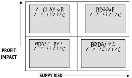
For the first time Kraljic [1] developed a conceptual model in order to determine the purchasing strategies for an organization based on parts' characteristics. This simple model is a two dimensional figure in which profit impact factor
has been allocated on the first side and supply risk factor on the other side. Several large companies like Shell, Alcatel, Philips, Akzo, Nobel and Siemens have applied this model. The survey by Boodie [12] illustrates that fifty percent of the purchasing management offices have implemented this model to establish their purchasing strategy, and eighty five percent of the managements have applied this concept to their organizations. Recently, the supply management subjects have been extended, and new issues have been introduced based upon Kraljic's work such as product development [13], supplier development [14], web-base procurement [15], engineering-purchasing interactions [16], change joint venture [17], and supplier segmentation [18]. Others like [19-30] also employed Kraljic model in their studies.
2. KRALJIC PERSPECTIVE ABOUT SUPPLY MANAGEMENT
situation the guaranty of the contract, supplier control, and strategy to keep enough inventory are recommended. Finally, the strategic items are the group of materials which needs a strategic/long-term relationship between buyer and supplier in order to maintain safe business. It is clear that different characteristics of the materials lead buyer to apply different methods of inventory control policies (Razmi and Ahmed [32]). In addition, buyer has different levels of authority and maneuver capability to buy particular materials (for detail discussion, please refer to Razmi and Karbasian [2]).
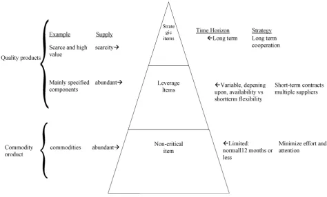
Based on a similar point of view, Dubios and Pederson [31] assigned four different criteria for the above four items (Routine items, Leverage items, Strategic items, and Bottleneck items). As it is illustrated in Figures 2 and 3, all items must be controlled by different policies and one should consider different criteria in order to have the optimal solution. The evaluation and selection
process differ depending on whether the product is classified as "quality" or "commodity". A quality product is one that is critical in the manufacturing process and needs hi-tech manufacturing techniques. These products are usually candidate for long-term supplier partnerships. A commodity product (or service) is generally non-critical in the manufacturing process and has a routine nature in market. Among the four categories introduced by Kraljic the leverage items and strategic items pose more motivation to optimize compared to the other two categories of routine items and bottleneck items since they encompass tremendous impact on profit. As Razmi and Karbasian have illustrated [2], the leverage items outlet with more suppliers compared to strategic items and also more value compared to total finished products. Therefore, they are still in strategic position. However, buyer should search for the best bargain and consider price as the most important criterion for long term contracts. In this situation, buyer should make sure that the quality of the materials and batches of materials received are in a regular manner. It must be mentioned that because of the important role of these items in the company's products, the manufacturer must be on its suppliers' performance list otherwise all production, distribution, and marketing plans will be faced with big challenges. Therefore, motivation to assess the suppliers and optimizing the purchasing schedule from the candidate suppliers is more apparent for leverage items. Due to little impact on supply risk in leverage items, there is more room to maneuver for optimization of the purchased items. As a result, in order to complete the idea introduced by Razmi and Karbasian [2] at the first step, the study is focused on optimizing procurement plan for leverage items. In this paper, two mathematical models are introduced for leverage items in order to solve supplier selection problem. The first model is a goal programming that considers deterministic condition and includes the following primary goals:
Minimizing net price, net rejection, and on time deliveries in a dynamic mode subject to the constraints regarding buyer's demands, vendor's capacity, and the buyer's limitations on budget, quality, on time delivery, etc. This model considers vendor selections for multiple items, multiple time periods and multiple sourcing.
LEVERAGE ITEMS
STRATEGIC
ITEMS
BOTTLENECK
ITEMS ROUTINE
ITEMS
PROFIT IMPACT
SUPPY RISK
Figure 1. Classification of the purchasing items by Kraljic.
MATERIALS
MANAGEMENT
SUPPLY
MANAGEMENT
SOURCING
MANANGEMENT PURCHASING
MANAGEMENT PROFIT
IMPACT
SUPPY RISK
The second model is a goal programming in probabilistic condition which includes the following primary goals:
Minimizing purchasing cost, rejection, and late deliveries (tardiness) subject to constraints regarding buyer's demand, vendor's capacity, and buyer's limitations on budget, quality, delivery time, etc.
3. SUPPLIER SELECTION IN DETERMINISTIC CONDITION
First of all, consider the following notations used in this paper.
Assumptions:
Demand of the item is constant and known with certainty.
Every supplier must supply at least one item.
Multiple sourcing, multiple items, multiple time periods are considered.
Indices:
i: index for product, for all i=1…..n j. index for supplier for all j=1…..si
t. index for time Variables:
Xijt: is a zero/one variable that shows the allocation of purchased ith item from jth
supplier in period t
Yijt: percent of Dit assigned to jthsupplier over a
period t. Parameters:
Dit: demand of ithitem in period t(constant).
Cijt: jth supplier's capacity for supplying the ith
item in period t.
qia: minimum acceptance rate of incoming ith
item (constant for all time periods)
qijt: acceptance rate of jth supplier for ith item in
period t.
Pijt: price of jthsupplier for ithitem in period t.
Si: number of candidates for purchasing ithitem.
Uit: maximum accepted earliest due date rate for ith item in period t. (It is known and
constant)
Kit: maximum accepted delay time rate for ith
item in period t. (It is known and constant) Mijt: earliest due date or delay time rate of jth
supplier for ithitem in period t.
3.1. Constraints The most important constraints of the problem are buyer's demand and quality, supplier capacity and lead time. These constraints are formulated as follows:
3.1.1. Capacity constraint The vendor j can provide up to cjunits of the product over a period t. Therefore:
YijtDit
Cijt for all i, j, t (1)3.1.2.Demand constraint Demand is equal to Dit and it is assumed that Si vendors can meet the buyer's demand, then:
it D it D i s j ijt Y 1
for all i, t 1 1 i s j ijt
Y (2)
3.1.3. Quality constraint qia is minimum
acceptance rate of incoming ith item and qijt is
acceptance rate of jthsupplier for ithitem in period t
and purchased volume is YijtDit the quality constraint can be formulated as follow:
it D ia q i s j it D ijt q ijt Y
1 ia
q i
s
j ijtit
q ijt Y
1
(3)
3.1.4. Lead time constraint Uitis assumed as the
maximum accepted earliest due date rate for ith
item in period tand Kitis maximum accepted delay
time rate for ithitem in period t. Mijtis earliest due
date or delay time rate of jthsupplier for ithitem in
period t. Therefore, the lead time constraint can be formulated as follows:
j it D it K ijt Z it D it U ijt Z it D ijt Y ijt
M (1 ) (4)
rate delay time as assigned is if : 0 date due earliest as assigned is if : 1 ijt M ijt M ijt Z
It is obvious that if Xijt is zero, Yijt is also zero, and if Xijt is equal to 1, Yijt must be bigger than zero. Therefore, since Yijt cannot be more than 1, the following constraints can satisfy the above conditions: ) ( ) ( ijt X ijt Y ijt X ijt Y
for all i, j, t
Where
is always slightly greater than zero. 3.1.5. The final model) 2 ( 1
minzijtPijtYijtDititdpitijt dnijt (5)
YijtDit
Cijt i s j ia q t i dp t i dn t i q ijt Y it D ia q i s j it D ijt q ijt Y
1 1 1 1
1
for all i,t
1 1 i s j ijt
Y for all i,t
jZijtUitDit Zijt KitDit t ij dp t ij dn it D ijt Y ijt M
) 1 (
2 2
(6)
3.2. Numerical Example It is assumed that the
manager decides to minimize the purchasing cost for the leverage items in two periods by selecting and planning its suppliers. Tables 1- 4 illustrate the required information of the suppliers for these two periods.
TABLE 1. Supplier's Information in Period (1) for Item (A).
D11=1000, K11=0.7, U11=0.1, TB11=16000, q1a=0.92
Price Defect Free Rate Mijt Capacity
Sup.1 9 0.92 0.6 (delay time rate) 600
Sup.2 12 0.95 0.4 (earliest due date rate) 700
Sup.3 14 0.98 0.4 (delay time rate) 500
TABLE 2. Supplier's Information in Period (2) for Item (A).
D12=800, K12=0.5, U12=0.4, TB12=16800, q1a=0.92
Price Defect Free Rate Mijt Capacity
Sup.1 22 0.95 0.5 (Delay Time Rate) 400
Sup.2 20 0.92 0.0 (on-time) 600
Sup.3 18 0.90 0.4 (Earliest Due Date Rate) 700
TABLE 3. Supplier's Information in Period (1) for Item (B).
D21=500, K13=0.2, U21=0.1, TB21=15000
Price Defect Free Rate Mijt Capacity
Sup.4 4 0.93 0.6(Delay Time Rate) 400
Sup.5 6 0.96 0.0 (on-time) 300
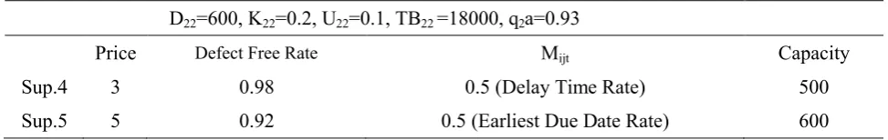
TABLE 4. Supplier's Information in Period (2) for Item (B).
D22=600, K22=0.2, U22=0.1, TB22=18000, q2a=0.93
Price Defect Free Rate Mijt Capacity
Sup.4 3 0.98 0.5 (Delay Time Rate) 500
3.2.1. Review of the cases By evaluating the suppliers, it can be understood that for item (A), there are 8 combinations of assigning suppliers of which only four possibilities should be evaluated, since other combinations are not feasible. Regarding item (B), there are 4 combinations of
assigning suppliers of which only two possibilities must be assessed.
Tables 5-8 illustrate the above facts and show the feasible allocation situations. Regarding Tables 5-8, we have 64 feasible combinations (4*4*2*2=64) to calculate the optimal solution.
TABLE 5. Zero/ One Variables Represent Supplier Selection and Feasible Cases for Part 1 in Period 1.
Case X111 X121 X131 Capacity Feasible/ unfeasible
1 1 1 1 1800 Feasible
2 1 1 0 1300 Feasible
3 0 1 1 1200 Feasible
4 1 0 1 1100 Feasible
5 1 0 0 600 unfeasible
6 0 1 0 700 unfeasible
7 0 0 1 500 unfeasible
8 0 0 0 0 unfeasible
Case X112 X122 X132 Capacity Feasible/ unfeasible
1 1 1 1 1700 Feasible
2 1 1 0 1000 Feasible
3 0 1 1 1300 Feasible
4 1 0 1 1100 Feasible
5 1 0 0 400 unfeasible
6 0 1 0 600 unfeasible
7 0 0 1 700 unfeasible
8 0 0 0 0 unfeasible
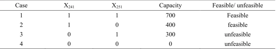
TABLE 7. Zero/ One Variables Represent Supplier Selection and Feasible Cases for Part 2 in Period 1.
Case X241 X251 Capacity Feasible/ unfeasible
1 1 1 700 Feasible
2 1 0 400 unfeasible
3 0 1 300 Feasible
4 0 0 0 unfeasible
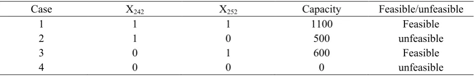
TABLE 8. Zero/ One Variables Represent Supplier Selection and Feasible Cases for Part 2 in Period 2.
Case X242 X252 Capacity Feasible/unfeasible
1 1 1 1100 Feasible
2 1 0 500 unfeasible
3 0 1 600 Feasible
4 0 0 0 unfeasible
The optimum answers for all situations are shown in Table 9. It can be seen from Table 9 that case 3 is an infeasible situation and case 1 has the minimum cost. Therefore, case 1 is the optimum solution for the above example with the minimum cost of 21752.03 money units. As it can be seen from the above example, the approach introduced in this paper can easily distinguish between feasible and infeasible situations of suppliers combinations. This is very important when we deal with the real cases in which practitioners face with numerous periods and suppliers. In addition, it is shown that for the first time the concept of budget constraint is put into purchasing plan in all individual periods of the purchasing plan.
3.2.2. Sensitivity analysis For the above example if demand changes to [D11=1200, D12=700,
D21=400, D22=500], Tables 5-8 will be modified as
follows. As it can be observed for item (A), there are 8 combinations of assigning suppliers in each period of time, which in periods one and two only three and five possibilities should be evaluated respectively, since the other combinations of assigning the suppliers are not feasible. Regarding item (B), there are 4 combinations of assigning suppliers which only two possibilities must be assessed. Tables 10-13 illustrate the above facts and show the feasible allocation situations. Regarding these tables we have 60 feasible combinations (5*3*2*2=60) to calculate the optimal solution. Table 14 illustrates the optimal result for this case. In the second period, if the proposed prices of suppliers 4 and 5 respectively change to 5 and 2 money units, we expect that the allocated purchased materials will be modified in favour of supplier 5. Based upon the above modification, the model is once again executed and the results are shown in Table 15 which illustrates logical answer to the above changes.
4. SUPPLIER SELECTION IN PROBABILISTIC CONDITION
The proposed second model attempts to minimize the cost of purchasing in probabilistic condition considering the following assumptions. It must be mentioned that solving the problem in the
probabilistic condition makes the second model more complicated and therefore, in this paper the elements of time has been excluded and the proposed model is not dynamic.
Assumptions:
(1) The periods of planning is known.
(2) The demand for each leverage items is known.
(3) The supply base (maximum number of suppliers) for all items is constant and known
Variables:
X
ij
: this is a zero/one variable that shows theallocation of purchased ith item from jth
supplier
Yij: the quantity of materials purchased from
supplier jif it has been selected Parameters:
Di: demand of ithitem (constant).
Cijt: jthsupplier's capacity for supply the ithitem
qij: failure rate of materials dispatched by
supplier jthforithitem (this is a random
variable with normal distribution)
qia: maximum acceptance rate of failure for ith
item (constant and known)
Lij: rate of tardiness related to jthsupplier which
has been selected to supply ith item that is a
random variable with normal distribution Lia: maximum acceptance rate of tardiness to
supply ith item which is a constant and
known
Pij: price of jthsupplier for ithitem
Fij: constant cost offer by supplier jfor procure
item i
TBP: total budget need to purchase all required items
l-A: probability of obtaining appropriate quality which is known
l-B: probability of delivering batch of materials in appropriate lead-time which is known
TABLE 9. Optimum Solution for Best of Cases.
Case Y111 Y121 Y131 Y112 Y122 Y132 Y241 Y251 Y242 Y252 Z
A 0.6 0.4 0 0 0.14 0.87 0.8 0.2 0.8 0.2 29048.02
TABLE 10. Zero/ One Variables Represent Supplier Selection and Feasible Cases for Part 1 in Period 1.
Case X111 X121 X131 Capacity Feasible/ unfeasible
1 1 1 1 1800 Feasible
2 1 1 0 1300 Feasible
3 0 1 1 1200 Feasible
4 1 0 1 1100 unfeasible
5 1 0 0 600 unfeasible
6 0 1 0 700 unfeasible
7 0 0 1 500 unfeasible
8 0 0 0 0 unfeasible
TABLE 11. Zero/ One Variables Represent Supplier Selection and Feasible Cases for Part 1 in Period 2.
Case X112 X122 X132 Capacity Feasible/ unfeasible
1 1 1 1 1700 Feasible
2 1 1 0 1000 Feasible
3 0 1 1 1300 Feasible
4 1 0 1 1100 Feasible
5 1 0 0 400 unfeasible
6 0 1 0 600 unfeasible
7 0 0 1 700 feasible
8 0 0 0 0 unfeasible
TABLE 12. Zero/ One Variables Represent Supplier Selection and Feasible Cases for Part 2 in Period 1.
Case X241 X251 Capacity Feasible/ unfeasible
1 1 1 700 Feasible
2 1 0 400 feasible
3 0 1 300 unfeasible
4.1.1. Being probable only for a single or multi-goal function in a multi-multi-goal problem:
n
j j ij
i x C x
f
1
~ )
( (7)
) 1
) ( (fi x bi
p [0,1] (8)
The above constraint could be a way to interfere the risk into the problem i.e. the more probable the above relation is (smaller the ), the more accessible bi (the time parameter of the goal
function) would be. is known and specified by the decision maker.
In this particular case, if the all distributions become normal, then the distribution fi(x)is
normal; hence:
1
2 1 ] ) ( [
1 )
~ (
x i f VAR
n
J j
X ij C E i
b z
p (9)
2 1 )] ( ( [
1 ) ~ (
X i f VAR
n
j j
X ij C E i
b
(10)
Since the accumulated normal function is absolutely ascending function, hence:
i b x
i f VAR j
X ij C E t s
n
j j
X ij C E x
i f E Optimum
2 1 ))] ( ( )[ ( 1 )
~ ( : .
1 ) ~ ( ))
( ( :
(11)
4.2. Constraints In this situation the most important constraints of the problem are: buyer demand, desired quality and lead-time, supplier capacity, supply base constraint and finally budget constraint. These constraints are formulated as follows:
TABLE 13. Zero/One Variables Represent Supplier Selection and Feasible Cases for Part 2 in Period 2.
Case X242 X252 Capacity Feasible/ unfeasible
1 1 1 1100 Feasible
2 1 0 500 unfeasible
3 0 1 600 Feasible
4 0 0 0 unfeasible
TABLE 14.Optimum Solution for Best of Cases.
Case Y111 Y121 Y131 Y112 Y122 Y132 Y241 Y251 Y242 Y252 Z
A 0.5 0.5 0.0 0.0 0.0 1.0 1.0 0.0 0.8 0.2 42916.01
TABLE 15. Optimum Solution for Best of Cases.
Case Y111 Y121 Y131 Y112 Y122 Y132 Y241 Y251 Y242 Y252 Z
4.2.1. Capacity constraint The vendor j can provide up to cjunits of the item i over period t. Therefore: ij X ij C ij
Y (12)
4.2.2. Quality constraint It is mentioned that the parameter of qia is a maximum acceptance failure
rate for ithitem. In this case, qijis the failure rate of
item ioffered by the jthsupplier. In this model qijis
a random variable with normal distribution.
A i S
j ij ij X
i S
j ij ij X ia q z P i S j A ia q ij q ij X P 1 2 1 1 2 2 1
1 ) 1
(
(13)
In the case of selection of the jthsupplier, Xij will be equal to 1, otherwise Xij=0 expressed as follows: ) 2 ( ) 1 ( 1 2 1 1 2 2 1 2 0 2 0 ) 1 ( A j S
j ij ij
X i S
j ij ij X ia q Z P ij X ij X ij X ij X ij X ij X (14) i S j ia q A M ij ij X A M i S
j ij ij
X ia q i S j M ij ij X
1 (1 )
1 ) 2 ( ) 1 ( 1 1 ) 2 ( 1 2 2 (15)
4.2.3. Number of vendors constraint The number of vendors is the most important decision for single/multi resource/s problems. In traditional era, manufacturers thought that increasing the number of vendors can decrease the risk of supply. However, today, it is believed that this idea is not proficient any more. In a sense, decreasing the number of vendors leads to the following benefits: 1) decrease the total cost of product, 2) procure from the best supplier/s, 3) utilize all supplier/s' facilities, 4) minimize the management cost and ease of implementation of developing supply policies, and 5) capability to develop supplier/s. Therefore, companies would like to optimize the number of vendors. This can be accomplished by introducing the model to capture all quantitative and qualitative parameters which affect the risk of supply. In this study we assumed that the maximum number of vendors cannot be more than T (a constant parameter). 4.2.4. Lead-time constraint As mentioned before, Liais a maximum acceptance tardiness rate
to supply ithitem, and Lijis the tardiness rate of the
supplier j regarding delivering ith item which is a
normal random variable. Hence, the following formula must be satisfied:
B i S
j ij ij
X i S
j ij ij X ia L z P i S j B ia L ij L ij X P 1 2 1 1 2 2 1 1 1 ) ( (16)
Since
Xij Xij
2 , like quality constraint we have:
i S j ia L B N ij ij X B N i S
4.3. The Final Model i S j m i ij X ij Y m i i S j TBP ij Y ij P i S j D ij Y m i i S j T ij X m i B i S j ia L ij L ij X P m i A i S j ia q ij q ij X P i S j m i ij X ij C ij Y m i i S j ij X ij F ij Y ij P Min ... 1 , ... 1 , * 10 ) 7 ( 1 1 ) 6 ( 1 ) 5 ( ... 1 1 ) 4 ( ... 1 , 1 1 ) 3 ( ... 1 , 1 1 ) 2 ( ... 1 , ... 1 , ) 1 ( 1 1 (18)
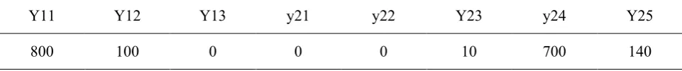
4.4. Numerical Example It is assumed that the manager decides to minimize the supply cost for two leverage items. The demand for the first item is 900, the maximum acceptance failure rate is 0.25, the maximum acceptance lead-time is 0.25, the probability of on-time delivery (1-B) is 0.75 and the probability of establishing the quality (1-A) is 0.75. The demand for the second item is 850, the maximum acceptance failure rate is 0.35, the maximum acceptance lead-time is 0.35, the probability of on-time delivery is 0.76, and the probability of establishing the quality is 0.76. Total budget for supplying these two items is 30,000 money units. The complementary information is illustrated in Tables 16 and 17. Furthermore, the optimal purchasing schedule proposed by the model is shown in Table 18. It is clear that in real situation, practitioners have to consider supplier/s development programs. This development can change the suppliers' situations and the practitioners do not need to wait and can highlight the future changes in their decisions.
As can be observed in Table 18, in both parts, suppliers with maximum total value are assigned.
TABLE 16.Supplier Information Regarding the First Item.
Constant cost Capacity Failure rate Tardiness rate Price 4 800 n (0.06,0.0036) n (0.065,0.0036) 5 Supplier No. 1
8 850
n (0.06,0.0049) n (0.065,0.0049)
7 Supplier No. 2
12 500
n (0.06,0.0016) n (0.065,0.0016)
9 Supplier No. 3
The maximum number of suppliers is 2 (T=2)
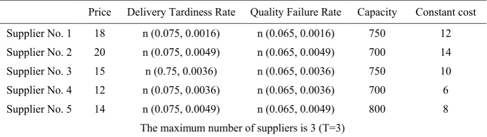
TABLE 17.Supplier Information Regarding the Second Item.
Constant cost Capacity
Quality Failure Rate Delivery Tardiness Rate
Price
12 750
n (0.065, 0.0016) n (0.075, 0.0016)
18 Supplier No. 1
14 700
n (0.065, 0.0049) n (0.075, 0.0049)
20 Supplier No. 2
10 750
n (0.065, 0.0036) n (0.75, 0.0036)
15 Supplier No. 3
6 700
n (0.065, 0.0036) n (0.075, 0.0036)
12 Supplier No. 4
8 800
n (0.065, 0.0049) n (0.075, 0.0049)
14 Supplier No. 5
The value is calculated based upon average of suppliers' quality, average of lead time, variance, proposed price, and finally the capacity of suppliers in each period of time. Using the above model, one can easily accomplish the sensitivity analysis by illustrating the results when faces with changes in suppliers' parameters or buyer's preferences.
4.4.1. Sensitivity analysis In the above numerical example l, first of all, we assumed that the capacity of suppliers 1 and 2 for supplying the first item changes from 800 to 900, and from 600 to 500 respectively. Also the capacity of suppliers 3 and 4 for supplying the second item changes from 700 to 850 and from 800 to 600 respectively. In this new
condition, the complementary information will be changed as shown in Tables 19 and 20. The optimal purchasing schedule for the recent changes is shown in Table 21. Suppose suppliers 1, 2, and 3 change their proposed price for the first item from 5 to 10, 7 to 8, and 9 to 6 money units respectively. In addition, suppose suppliers 3, 4, and 5 change their proposed price for the second item from 15 to 14, 12 to 16, and 14 to 12 money units respectively. Then for the first item, it is logical to expect increase in the share of supplier 3 and for the second item we should see an enhancement in supplier’s 5 purchased share. Therefore, the optimal solutions, shown in Table 22 confirm the rightness of the designed model.
TABLE 18. The Optimal Solution for These Two Leverage Items.
Y25 y24
Y23 y22
y21 Y13
Y12 Y11
140 700
10 0
0 0
100 800
TABLE 19. Supplier Information Regarding the First Item.
Constant Cost Capacity
Failure Rate Tardiness Rate
Price
4 900
n (0.06,0.0036) n (0.065,0.0036)
5 Supplier No. 1
8 750
n (0.06,0.0049) n (0.065,0.0049)
7 Supplier No. 2
12 600
n (0.06,0.0016) n (0.065,0.0016)
9 Supplier No. 3
The maximum number of suppliers is 2 (T=2)
TABLE 20. Supplier Information Regarding the Second Item.
Constant Cost Capacity
Quality Failure Rate Delivery Tardiness Rate
Price
12 750
n (0.065,0.0016) n (0.075,0.0016)
18 Supplier No. 1
14 700
n (0.065,0.0049) n (0.075,0.0049)
20 Supplier No. 2
10 650
n (0.065,0.0036) n (0.75,0.0036)
15 Supplier No. 3
6 850
n (0.065,0.0036) n (0.075,0.0036)
12 Supplier No. 4
8 600
n (0.065, 0.0049) n (0.075, 0.0049)
14 Supplier No. 5
5. CONCLUSIONS
Supplier selection is one of the most important aspects in supply chain management in which cost, quality, delivery performances, etc. should be considered. Based upon Kraljic finding, the characteristics of the required materials must be considered in addition to the capability and performance of the suppliers. Regarding this concept, all materials can be categorized into four categories of strategic, leverage, bottleneck, and routine items. Among these four groups of items leverage items possesses the highest motivation to optimize due to its share in profit impact and the potential for buyer maneuverability. This paper illustrates two mathematical models (goal programming) for leverage items in order to select the best supplier/s and procurement plan. In the first model supplier/s selection process is achieved in a dynamic state with the constant and deterministic rate of delivery tardiness and quality failure rate. The second model considers the selection of supplier/s and procurement of leverage items plan under risk condition. Furthermore, the second model studies the problem in a static state. It evaluates the situation considering rate of delivery tardiness and quality failure rate as probabilistic variables which is more realistic and close to practical circumstances. Both models are followed by relative numerical examples in order to illustrate how the proposed models work. In addition, sensitivity analyses are provided for both models.
For future research it is suggested to consider the cost parameter in more detailed structure. For example, in the developed model all costs are presented in one figure of material price. However, the cost factor can be divided into several aspects of transportation cost and ordering expenses. In
addition, in order to catch up lean production concept, one can ponder materials return cost into the model. Regarding the second model, the current model has a static viewpoint. Moreover, it is suggested to develop a dynamic mathematical model. In order to make the model easier to solve, the authors presumed the quality and lead time as random variables with normal distributions. It is recommended to consider other distributions in the model. Furthermore, it is recognized that due to difficulty in solving the probabilistic model by mathematical programming, the time factor has not considered in the second model. It is recommend applying meta-heuristic methods such as Genetic Algorithm, Ant-Colony, etc. to construct the dynamic approach.
Since the strategic items have also an important impact on benefit and the bottleneck items have very vital affects on supply risk, it is recommended to study and introduce the model to optimize the procurement plan for these two items as well. When practitioners deal with strategic items, they must make sure about progress in quality and delivery performances in the time horizon; since company cannot change the supplier very easily (this figure is totally different as we are dealing with leverage items). Therefore, the proposed model should guaranty this continuous development in the model parameters.
6. REFERENCES
1. Kraljic, P., “Purchasing Must Become Supply Management”, Harvard Business Review, Vol. 61, No. 5, (1983), 109-117.
2. Razmi, J. and Karbasian, S., “The Role of Expert Systems in Evaluating and Control of Suppliers in Various Purchasing Circumstances”, 3rd European Conference on Intelligent Management Systems in Operations, U.K., Manchester, (28-29 June 2005). 3. Neely, A.D. and Byrne, M.D., “A Simulation Study of
Bottleneck Scheduling”, International Journal of Production Economics, Vol. 26, (1992), 187-192. TABLE 21. The Optimal Solution for These Two Leverage Items.
Y25 y24
Y23 y22
y21 Y13
Y12 Y11
10 830
10 0
0 0
10 890
TABLE 22. The Optimal Solution for These Two Leverage Items.
Y25 y24
Y23 y22
y21 Y13
Y12 Y11
600 10
240 0
0 0
4. Ghobadian, A., Stainer, A., and Kiss, T., “A Computerized Vendor rating System Proceedings of the First International Symposium on Logistics”, Nottingham, U.K., (July 1993), 321-328.
5. Gaball, A.A., “Minimum Cost Allocation of Tender”, Operational Research Quarterly, Vol. 25, No. 3, (1974), 389-398.
6. Anthony, T.F. and Buffa, F.P., “Strategic Purchasing Scheduling”, Journal of Purchasing and Materials Management, Vol. 13, No. 3, (1977), 27-31.
7. Narasimhan, R. and Stoynoff, K., “Optimising Aggregate Procurement Allocation Decisions”, Journal of Purchasing and Materials Management, Vol. 22, No. 1, (1986), 23-30.
8. Razmi, J., Rafiei, H., and Hashemi, M., “Designing a Decision Support System to Evaluate and Select Suppliers using Fuzzy Analytic Network Process”, Computers and Industrial Engineering, Vol. 57, No. 4, (2009), 1282-1290.
9. Rosentha, E.C., Zodyak, J.L., and Chaudhry, S.S., “Vendor Selection with Bundling”, Decision Science, Vol. 26, No. 1, (1995), 35-48.
10. Ghodsypour, S.H. and O’Brien, C., “The Total Cost of Logistics In Supplier Selection, Under Conditions of Multiple Sourcing, Multiple Criteria and Capacity Constraints”, International Journal of Production Economics, Vol. 73, (2001), 15-27.
11. Razmi, J. and Rafiei, H., “An Integrated Analytic Network Process with Mixed Integer Non-Linear Programming to Supplier Selection and Order Allocation”, International Journal of Advanced Manufacturing Technology, Vol. 49, (2009), 1195-1208.
12. Boodie, M.L.J., “World Class Purchasing in Nederland is Fictie en Helaas Nog Geen Werkelijkheid”, Berenschot Inkoopenquête, Berenschot Inkoop Management, (1997). 13. Wynstra, J.Y.F. and Ten Pierick, E., “Managing
Supplier Involvement in New Product Development: A Portfolio Approach”, European Journal of Purchasing and Supply Management, Vol. 6, No. 1, (2000), 49-57. 14. Handfield, R.B., Krause, D.R., Scannell, T.V. and
Monczka, R.M., “Avoid the Pitfalls in Supplier Development”, Sloan Management Review, Vol. 41, No. 1, (2000), 37-49.
15. Croom, S.R., “The Impact of Web-Based Procurement on the Management of Operating Resources Supply”, The Journal of Supply Chain Management, Vol. 36, No. 1, (2000), 4-13.
16. Nellore, R. and Taylor, J.E., “Using Portfolio Approaches to Manage Engineering-Purchasing-Supplier Interaction”, Production and Inventory Management, Vol. 41, No. 1, (2000), 6-12.
17. Axelsson, B., Frisk, K. and Najib, A., “From Buying To Supply Management–A Multifaceted Change Venture”,
Proceedings of the 9th International IPSERA
Conference, London, Canada, (2000), 55-66.
18. Moller, M. and J. Momme, “Supplier Segmentation in Theory and Practice–Towards A Competence Perspective”, Proceedings of the 9th International
IPSERA Conference, London, Canada, (2000), 508-519.
19. Gelderman, C.J. and Van Weele, A.J., “Advancements in the use of a Purchasing–Portfolio Approach: A Case Study”, Proceedings of the 10thInternational IPSERA Conference, Jnkping, Sweden, (2001), 403-415. 20. Gelderman, C.J. and A.J. van Weele, “Strategic
Direction through Purchasing Portfolio Management: A Case Study”, International Journal of Supply Chain Management, Spring, Vol. 38, No. 2, (2002), 30-37. 21. Ahman, S., “Strategic Sourcing of Suppliers in a Supply
Network”, Proceedings of the 11th International IPSERA Conference, Enscheda, Netherlands, (2002), 1-10.
22. Dubois, A. and Pedersen, A.C., “Why Relationships do Not Fit into Purchasing Portfolio Models–A Comparison Between the Portfolio and Industrial Network Approaches”, European Journal of Purchasing and Supply Management, Vol. 8, No. 1, (2002), 35-42. 23. Olsen, R.F. and Ellram, L.M., “A Portfolio Approach to
Supplier Relationships”, Industrial Marketing Management, Vol. 26, No. 2, (1997), 101-113.
24. Zolkiewski, J. and Turnbull, P., “Relationship Portfolios –Past Present and Future”, Proceedings of the 16th Annual IMP Conference, Bath, United Kingdom, (2000).
25. Nellore, R. and Sdِerquist, K., “Portfolio Approaches to Procurement Analyzing the Missing Link to Specifications”, Long Range Planning, Vol. 33, No. 2, (2000), 245-267
26. Wynstra, J.Y.F., “Purchasing Involvement in Product Development, Doctoral thesis, Eindhoven Centre for Innovation Studies”, Eindhoven University of Technology, (1998).
27. Gelderman, C.J., “Rethinking Kraljic: Towards A Purchasing Portfolio Model, Based on Mutual Buyer-Supplier Dependence”, Danish Purchasing and Logistics Forum, Vol. 37, No. 10, (2000), 9-15. 28. Bensaou, M., “Portfolios of Buyer-Supplier
Relationships”, Sloan Management Review, Vol. 40, No. 4, (1999), 35-44.
29. Lilliecreutz, J. and Ydreskog, L., “Supplier Classification as an Enabler for A Differentiated Purchasing Strategy”, Global Purchasing and Supply Chain Management, (November, 1999), 66-74.
30. Olsen, R.F. and Ellram, L.M., “A Portfolio Approach to Supplier Relationships”, Industrial Marketing Management, Vol. 26, No. 2, (1997), 101-113.
31. Dubois, A. and Pedersen, A.C., “Why Relationships do not Fit into Purchasing Portfolio Models–A Comparison Between the Portfolio and Industrial Network Approaches”, European Journal of Purchasing and Supply Management, Vol. 8, No. 1, (2002), 35-42. 32. Razmi, J. and Ahmed, P.K., “Use of A Modified Analytic