OPTIMIZATION OF HEAT TRANSFER ENHANCEMENT OF A
FLAT PLATE BASED ON PARETO GENETIC ALGORITHM
M. Kahrom* , P. Haghparast and S. M. Javadi
Department of Mechanical Engineering, Ferdowsi University of Mashhad, Mashhad, Iran, [email protected] , [email protected] , [email protected]
*Corresponding Author
(Received: October 2, 2009 – Accepted in Revised Form: May 20, 2010)
Abstract A quad inserted into a turbulent boundary layer of a flat plate and its effect on average heat transfer and the friction coefficient is studied. To optimize this effect, the edge sizes and distance of the quad from the flat plate are continually modified. In each case, simultaneously the heat transfer enhancement and reduction in skin friction are analyzed. For optimization, the genetic algorithm technique is employed and the results of each step of progress studied by following the Pareto curves.
Physical domain is divided into control volumes, over which flow equations are discretized. To deal with the turbulence, several turbulence schemes are examined and appearance of flow features and
stability in hard environments are monitored. The turbulence model proved to give
reliable solutions and stability to all the 1,600 cases under consideration. Based on the Pareto curve
and with no single exceptions of the cases studied, results show that as the heat transfer coefficient rises, the skin friction falls simultaneously; in other words, there is an inverse relation between heat transfer enhancement and skin friction. Conclusion also made that the rate of heat transfer enhancement is more sensitive to modification on small area quads than those of large ones. Since the experimental validation of too many cases was impractical, random comparison between some numerical results and wind tunnel experiments is performed. The comparison showed that the numerical results are strongly in agreement with the experiments.
Keywords Genetic Algorithm, Pareto Front, Heat Transfer Enhancement, Reynolds Analogy
ﻩﺪﻴﻜﭼ
ﺖﻨﻟﻮﺑﺭﻮﺗ ﻱﺯﺮﻣ ﻪﻳﻻ ﻞﺧﺍﺩ ﻪﺑ ﺵﻮﮔ ﺭﺎﻬﭼ ﻚﻳ ﺩﻭﺭﻭ ﺮﺛﺍ ﻱﻭﺭ ﺮﺑ
ﻝﺎﻘﺘﻧﺍ ﺐﻳﺮﺿ ﺶﻳﺍﺰﻓﺍ ﺮﺑ ﺖﺨﺗ ﻪﺤﻔﺻ ﻚﻳ
ﺩﻮﺷ ﻲﻣ ﻲﺳﺭﺮﺑ ﺕﺭﺍﺮﺣ .
ﻡﺮﮔ ﻪﺤﻔﺻ ﺢﻄﺳ ﺯﺍ ﻥﺁ ﻪﻠﺻﺎﻓ ﻭ ﺵﻮﮔﺭﺎﻬﭼ ﻉﻼﺿﺍ ﻩﺯﺍﺪﻧﺍ ،ﺕﺭﺍﺮﺣ ﻝﺎﻘﺘﻧﺍ ﺐﻳﺮﺿ ﻥﺩﺮﻛ ﻪﻨﻴﻬﺑ ﻱﺍﺮﺑ
ﻙﺎﻜﻄﺻﺍ ﺐﻳﺮﺿ ﻭ ﺕﺭﺍﺮﺣ ﻝﺎﻘﺘﻧﺍ ﺐﻳﺮﺿ ﺮﻴﻴﻐﺗ ﺖﻟﺎﺣ ﺮﻫ ﺭﺩ ﻭ ﻩﺪﺷ ﻩﺩﺍﺩ ﺮﻴﻴﻐﺗ ﺕﺎﻌﻓﺩ ﻪﺑ ،ﻥﺁ ﺭﻭﺎﺠﻣ ﺖﺳﺍ ﻩﺪﺷ ﻞﻴﻠﺤﺗ
.
ﺯﺍ ﻥﺩﺮﻛ ﻪﻨﻴﻬﺑ ﻱﺍﺮﺑ ﻲﻣ ﻝﺎﺒﻧﺩ ﻮﺗِﺮَﭘ ﻱﺎﻫ ﻲﻨﺤﻨﻣ ﻱﻭﺭ ﺮﺑ ﻪﺴﻳﺎﻘﻣ ﺮﻫ ﻪﺠﻴﺘﻧ ﻥﺁ ﺭﺩ ﻪﻛ ﺩﻮﺷ ﻲﻣ ﻩﺩﺎﻔﺘﺳﺍ ﻚﻴﺘﻧﮊ ﻢﺘﻳﺭﻮﮕﻟﺍ ﺵﻭﺭ
ﺩﻮﺷ . ﻱﺎﻫ ﻝﺪﻣ ﻭ ﻩﺪﺷ ﻲﻠﺿﺎﻔﺗ ﺎﻫ ﻢﺠﺣ ﻦﻳﺍ ﻱﻭﺭ ﺮﺑ ﻥﺎﻳﺮﺟ ﺕﻻﺩﺎﻌﻣ ﻭ ﻢﻴﺴﻘﺗ ﻲﻟﺮﺘﻨﻛ ﻱﺎﻫ ﻢﺠﺣ ﻪﺑ ﻲﻜﻳﺰﻴﻓ ﻱﺎﻀﻓ ﺍﺪﺘﺑﺍ
ﻪﺘﻓﺮﮔ ﺭﺍﺮﻗ ﺏﺎﺨﺘﻧﺍ ﻭ ﻥﻮﻣﺯﺁ ﺩﺭﻮﻣ ﻲﺴﻨﻟﻮﺑﺭﻮﺗ ﻒﻠﺘﺨﻣ ﺖﺳﺍ
. ﺪﺷ ﻪﻈﺣﻼﻣ ﻝﺪﻣ ﻪﻛ ﺖﺳﺍ ﻩ
ﻱﺎﻫ ﺦﺳﺎﭘ ﻱﺮﺘﻬﺑ
ﺭﺩ ١٦٠٠ ﺪﻫﺩ ﻲﻣ ﺖﺳﺩ ﻪﺑ ﻪﻌﻟﺎﻄﻣ ﺩﺭﻮﻣ .
ﺐﻳﺮﺿ ﺶﻳﺍﺰﻓﺍ ًﻻﻭﺍ ﻪﻛ ﺩﻮﺷ ﻲﻣ ﻩﺪﻳﺩ ﺎﻨﺜﺘﺳﺍ ﻥﻭﺪﺑ ﻭ ﻮﺗِﺮَﭘ ﻱﺎﻫ ﻲﻨﺤﻨﻣ ﺱﺎﺳﺍ ﺮﺑ
ﻂﺳﻮﺘﻣ ﺕﺭﺍﺮﺣ ﻝﺎﻘﺘﻧﺍ
ﻩﺭﺍﻮﻤﻫ
ﺖﺳﺍ ﻩﺍﺮﻤﻫ ﻙﺎﻜﻄﺻﺍ ﺐﻳﺮﺿ ﺶﻫﺎﻛ ﺎﺑ
. ﻲﻨﻌﻳ ﻭﺩ ﻦﻳﺍ ﺕﺍﺮﻴﻴﻐﺗ ﻪﺼﺨﺸﻣ
ﺖﺒﺴﻧ ﺮﮕﻳﺪﻜﻳ ﺎﺑ
ﺭﺍﺩ ﻪﻧﻭﺭﺍﻭ ﺪﻧ .
ﺮﻴﻴﻐﺗ ﻪﺑ ﺮﺗ ﺱﺎﺴﺣ ﺵﻮﮔ ﺭﺎﻬﭼ ﻚﭼﻮﻛ ﻱﺎﻫ ﻊﻄﻘﻣ ﺢﻄﺳ ﻱﺍﺮﺑ ﺕﺭﺍﺮﺣ ﻝﺎﻘﺘﻧﺍ ﺐﻳﺮﺿ ﺶﻳﺍﺰﻓﺍ ًﺎﻴﻧﺎﺛ
ﻩﺯﺍﺪﻧﺍ
ﺖﺣﺎﺴﻣ ﻩﺩﻮﺑ ﺖﺳﺍ . ﻲﻫﺎﮕﺸﻳﺎﻣﺯﺁ ﺞﻳﺎﺘﻧ ﺎﺑ ﻭ ﻡﺎﺠﻧﺍ ﻱﺩﺪﻋ ﻱﺎﻫ ﻞﺣ ﺯﺍ ﻲﻓﺩﺎﺼﺗ ﺶﻨﻳﺰﮔ ،ﻱﺩﺪﻋ ﺞﻳﺎﺘﻧ ﻲﺠﻨﺳ ﺖﺤﺻ ﻱﺍﺮﺑ
ﺖﺳﺍ ﻩﺪﺷ ﻪﺴﻳﺎﻘﻣ .
ﻪﺴﻳﺎﻘﻣ ﺎﺑ ﺍﺭ ﻲﺑﻮﺧ ﻕﺎﺒﻄﻧﺍ ﺞﻳﺎﺘﻧ
ﻲﻣ ﻥﺎﺸﻧ ﻲﻫﺎﮕﺸﻳﺎﻣﺯﺁ ﺪﻨﻫﺩ
.
1. INTRODUCTION
The growing demands to extract heat from limited areas prompts engineers to develop techniques to enhance the heat transfer coefficient. One of the old methods is to augment turbulent intensity in the boundary layer by roughening the surface and stimulating turbulent heat transfer, [1]. Another method similarly suggests that the application of
placed inside a turbulent boundary layer of a flat plate and the amount of heat transfer enhancement is measured at 60%, when compared to a single flat plate without the insert. In all of these methods, the amount of heat augmentation is tempting even though the risk of increasing in skin friction leaves only a limited era to employ these techniques. Inaoka et al. [6] placed an insert into the turbulent boundary layer and measured both the heat and skin friction coefficients along the affected area. Amazingly, the results violated the Reynolds Analogy between heat and momentum transfer in that the insert was a cause of heat transfer enhancement (HTE), the skin friction also happened to be reduced simultaneously. More studies by Teraguchi et al. [7] and Kong et al.[8] also reported the same type of violation of the Reynolds Analogy. If result is proved to be sustainable in similar stimulations of the boundary layer, this would highlight the unique advantage of an insert for HTE.
The present work insists on maximizing the heat transfer coefficient, while the skin friction is constantly minimized and the blockage effect by an obstacle also diluted. Therefore, the problem is one of three objectives optimization.
The optimization of multi-objective functions that are in conflict with each other is best handled by the multi-objective Genetic Algorithm. This method has gained popularity in fluid dynamics and thermal flow optimization during the last decade [9].
MacCormac et al. [10] employed the Genetic Algorithm (GA) to optimize suction distribution over a flat plate in order to delay transition and therefore reduce the friction drag. Leng et al. [11] used GA to optimize the design of a small flying object and so achieved optimized lift and drag forces on the body. Tiwary et al. [12] analyzed the effect of splitter on stabilizing lift and drag forces acting on a circular cylinder. Amanifard et al. [13] employed multi-objective GA and a neural network to optimize heat flux from a rectangular cylinder at R D 1400. The cylinder was placed at different distances from a flat plate and the effect of distances on the Strouhal number and lift was studied. More applications of GA on the optimization of heat transfer devices are reported by Xie et al. [14], Gholap et al. [15] and Hilbert et al. [16].
In literature, the word "genetic algorithm" was initially introduced by Bagley et al. [17], who published the first application of GAs. While most of the early works on GAs are attributed to Holland[18], De Jong [19], and Goldberg [20], who made significant advancements in GAs, during the 1980s, but the interest in the utilization of GAs in the field of numerical heat transfer is quite recent. This is probably due to the fact that most numerical problems are time consuming and several simulations must be performed. Nevertheless, Goldberg [20] reports that GAs began to be used more cautiously in heat transfer in approximately the mid-1990s and have recently became increasingly more trustworthy. After a modest annual increase in the number of papers during the first decade of the millennium, GAs appear to be a promising and accessible alternative for the optimization in thermal systems.
Basically, the GA idea applies an analogy of the evolution theory, by which so-called decision variables or genes of a generation are manipulated by using various operators (acting here as crossovers or mutations) in order to create newly designed population, that is, new sets of decision variables for further evolution.
The present work concentrates on the effect of a quad type insert on the disturbance of a turbulent boundary layer and, as a consequence, the effects on the heat transfer of the neighboring flat plate. Emphasis is placed on the quad's shape on the maximization of the heat transfer coefficient, h , while minimization of skin friction, C and reduction of the blockage effect are also considered. A description of the physical domain is first given.
2. PROBLEM DEFINITION
Air flows at 20 ° parallel to a flat plate which is at a
constant surface temperature of 70 ° . At
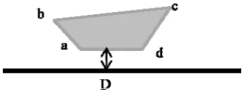
1400 from the leading edge, at which 1.63 10 , a quad is inserted into the turbulent boundary layer. Depending on the quad shape and its distance from the flat plate, the deformation of the boundary layer is specified, thus creating a specific distribution of the heat and friction coefficients over the flat plate for each configuration.
presented in Figure 1. By optimization, the coordinates of four corners a, b, c and d of the quad are changed until the optimal group of shapes and their distances (D) from the flat plate is reached.
To facilitate the comparison between many different cases of studies, an affected area is defined as the area of the flat plate on which the local heat transfer coefficient is stimulated by 5% of that of a single flat plate with a similar but undisturbed flow condition.
Figure 1. A sample quad located in a turbulent boundary layer of a flat plate.
3. OPTIMIZATION BY GA
GA is based on an analogy with the evolution theory, i.e. the inevitable course of nature. Alike in nature, an original population of individuals is manually created and represents a primitive generation of parents. Each individual's fitness is first determined by how well that individual adapts to a given environment and then evaluated by how well that individual survives. Fit individuals go through a process of survival solution, crossover and mutation which results in the creation of the next generation of individuals, indeed the children individuals. Who are formed from a selection of optimum individuals that is parents and children. Since solution algorithms are relatively different for GAs, it is important to distinguish between single-objective and objective GAs. In multi-objective GAs, as is in this study, the aim is to find many non-dominated solutions, whose per-formance spreads over the objective functions domain, known as the Pareto front. According to Pareto's rule, the individual A dominates the individual B if, for at least one of the objectives, A is clearly better adapted than B and if, for all other objectives, A is no worse than B. An objective is considered optimal if it is non-dominated in the sense of this rule.
To each of the individuals, a rank number is
devoted that is equal to the number of individuals dominating it. If an individual is not dominated by any other, it is given the top ranking number, the numeral one. An individual which is dominated by individuals receives the rank 1. Non-dominated individuals always have a rank of one. At the end, the best individuals are all the non-dominated individuals throughout all generations, leading to what is called the Pareto front. This rule classifies the individuals of the population, inorther to calculate the corresponding fitness values, [16].
In each step of the solution, the objective vector is called the Pareto-optimal if and only if there is no feasible solution that dominates this solution vector. These Pareto-optional solutions form the Pareto front.
4. MULTI-OBJECTIVE VARIABLES
To formulate the problem, a vector variable is considered as genes in:
, , … (1)
When applying the vector function
, , (2)
maps onto an objective vector as:
, , … (3)
More specifically for the present case, the elements of vector are coordinates of four varying vertices of the quad, namely vertices a, b, c and d of the quad as are shown in the Figure 1:
, … , …
, , , , , , ,
(4)
To calculate the local heat transfer coefficients there is:
0.
/ / 0.
(5)
so for the friction coefficient:
/
(6)
Finally, the averaged heat and friction coefficients over the affected area are:
, ∆ ,
/
-(7)
and:
,
∆ (8)
The area of the quad is responsible for the flow blockage and has to be minimized in this optimization:
A f x ,
(9)
Values of , and are components of the objective vector , , . Constraint must be exercised to keep variables within reasonable ranges.
5. CONSTRAINTS AND LIMITATIONS
In producing each generation, constraints and limitations are imposed to keep primitive variables and objectives within the defined ranges. Table 1 shows limitations to keep the quad inside the boundary layer and in a position where remains constant as specified before. Here, coordinates of four vertices are the basic elements of the constraint vector. Numerically, these are specified in Table 2. Other variables, and
, are consequences of solutions of flow equations around the newly formed quad.
Table 1. Limitations imposed on vertices of the quad
Coordinates of: 1400 1410 ,
1.0 9.8
1400 1414,
2.2 12
c 14062.2 12 1420,
1406 1420,
1.40 9.8
1.0 9.8
Table 2, Constraints imposed on geometrical imitations.
1 2
3 ,
4
By imposing these constraints, quad edges remain within agreed physical ranges:
In all cases of examination, the whole body of the quad remains inside the boundary layer.
One of the edges of the quad is always kept parallel to the flat plate.
None of edges is eliminated in optimization. GA, in its first step, assumes a primitive population ( ), which is formed by using arbitrary design variables in the permitted range of values. Each set of adopted variables defines a member of a generation. In the next step, based on the results for the first generation's objective vector, the same technique is employed to assign populations for the next generation. The following are parameters defining the decision making:
Population size, Generation,
Crossover probability, Mutation probability, Selection strategy.
modifies individual genes to obtain the next generation individuals. Once a population is initiated, it is sorted based on domination reasoning; the first front is completely non-dominated in the current population and the second front (the next generation) is dominating individuals of the first front, and so on.
An algorithm decides how to choose transcendence members from the present generation to motivate the next generation. The odds assigned to each member to advance to next generation are:
p f
∑ f (10)
where f is the transcendence of the member in the generation.
The production of each member of a generation is assumed to be a function of the crossover probability and the mutation probability function . The size of the population must be large enough to achieve a better selection in shorter sequences. However, by increasing the number of the population, the amount of calculation increases and so lowers the rate of convergence. Since the selection strategy is based on probability, there is no guarantee of arriving at a better combination of population in the next generation. There is also a chance of diverging from the optimized target, [9].
6. GOVERNING EQUATIONS AND NUMERICAL METHOD
The dynamics of two dimensional incompressible flows over a flat plate which has been disturbed by a quad is governed by conservation equations of mass and momentum, namely the Navier-Stokes equations, which is expressed by:
The continuity:
m i
i R
x u
( )
(11) The momentum:
ρu ∂u
∂x
∂p ∂x
µ ρú ú R (12)
and the energy equations:
ρ u T µ
P
T ρ T′u′ R
T (13)
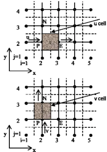
The numerical method is based on the control-volume formulation. The physical domain is divided into control volumes. Each control volume is associated with a discrete point at which dependent variables, such as velocity, pressure and temperature, are to be calculated. Discretization equations are derived by integrating the equations 11 to 13 over these control volumes. Figure 2 shows a sample rectangular computational domain subdivided into such control volumes. In this figure, the dashed surfaces denote the control volume.
Figure 2. Momentum control volumes
The two sides of the control volume on grid are the faces to count for upstream momentum and the component of velocity at . The top and bottom surfaces are similarly employed for the calculation of component of the velocity.
temperature are at the cell centre.
A first order implicit scheme is employed for discretising the time derivatives. Pressure is linked between the continuity and momentum equations. Finally, by calculating the density and velocity components, the energy equation is solved.
A single iteration consists of the sequential solution of equations in the following steps:
1. Implicitly solving the momentum equation for and
2. Solving the continuity equation for pressure correction using the successive under relaxation method
3. Solving the energy equation to achieve new values for temperature
4. Updating the velocity components, pressure, density and temperature for each grid point
The solution for each iteration results in the values for variables at the end of a time step. Values at the next time step are based on the solution of the previous iteration:
Δt. R R R RT
in which
u v p T
The operator acts as an "or" operator. Then, is either one of the variables u, v, ρ or T, as R , R , R and RT are residuals in relevant equations, respectively. The iterative solution is carried on until a stable repetitive flow is reached. However, the convergence criteria of Max
/ 10E 04 is applied to all variables at the end of each iteration.
In equation 12, the turbulent Reynolds stresses,
ρ u u , are to be calculated for closure by an
appropriate turbulence model. Two-equation turbulence models are generally superior to the zero and one equation models. These turbulence models do not require prior knowledge of the turbulence structure. They predict most industrial flows well and are reliable in stability and time consumption. In these models, the Reynolds stresses are assumed to be linearly proportional to the strain rate as calculated for molecular viscosity:
ρ u u µ ρ k δ (14)
µ is the turbulent eddy viscosity, δ is the Kronecker delta, and k u u is the kinetic
energy of turbulence. The eddy viscosity, in turn, is obtained from an empirical formula as a function of the kinetic energy of turbulence and the turbulence length scale. In the standard k
model, originally developed by Launder and Spalding and latter is referred to by Davidson [21], the transport equations for the kinetic energy of turbulence, k, has been proven to be:
ρu µ µ P ρ (15)
and the time rate of dissipation is defined as:
µ
ρ ∂u ∂x⁄ ∂u ∂x⁄ (16)
A turbulence length scale, l, relates k and :
l k / (17)
Once and are obtained from the solution of their respective transport equations, the eddy viscosity can be calculated from µ ρ Cµ k , where, Cµ is an empirical constant.
When using two-equation models, the equation is usually the first choice while there are varying ideas among users in choosing the second equation for each flow field. In this work, besides the 1,600 dissimilar cases of flow fields that must be evaluated without a single failure due to either the instability or malfunction in accuracy of the numerical scheme, the calculation speed throughout the total work must also be conceived. To choose a turbulence model suitable to handle the challenging environment of the present work, the standard k , RNG k , Realizable k
flow conditions from low (near the wall) to high Reynolds numbers (away from the wall).
Here the RNG k is accepted as the turbulence model. The dissipation equation [22] then reads as:
u ∂
∂x C kν s C k R
ανT (18)
Where ν Cμ in which Cμ 0.0845,
νT ν ν ,and
R Cμη 1 η η⁄
1 βη k (19)
where β 0.012, η 4.38 are constants and
η S k/ is defined when S 2S S and the magnitude of the strain rate is:
S ∂u ∂x⁄ ∂u ∂x⁄ ⁄2 (20)
The RNG theory gives values of constants
C 1.42, C 1.68, and α 1.39. The inverse turbulent Prandtl number, α , differs from that of the standard k model, α 1. Indeed the value of α derived by the RNG scalar heat transfer relation is:
α 1.3929
α 1.3929
. α 2.3929
α 2.3929
.
α νT
(21)
For the heat transfer problems α refers to the molecular inverse Prandtl number. In regions of small η, the value of R tends to somewhat increase eddy viscosity and in regions of very large η, where strong anisotropy exists, R can become negative and reduce eddy viscosity even more. This feature of the RNG model holds the most attraction in that it marked improvement in anisotropic large-scale eddies [22]. While the standard k ε model is a high Reynolds number model, the RNG theory provides an analytically-derived differential formula for effective viscosity that accounts for low Reynolds number effects as well. The efficacious use of this feature, however, depends on appropriate treatment of the near-wall refinement, assuming the location of the first grid point off the wall is inside of the sub-layer. The
turbulent heat flux, ρT′u′ , in Equation 13 is
obtained according to the simple gradient diffusion:
ρT′u′ μ σ
∂T
∂x (22)
where σ is the turbulent Prandtl number whose value is given as 0.85.
7. GRID GENERATION AND CODE VERIFICATION
Grid point distribution in a computational domain is non-uniform. Unlike a single flow field examination that is the subject of much research work, the present work is comprised of 1,600 different compositions of a quad and a flat plate boundary layer that must be re-meshed and resolved sequentially. It is difficult to address a precise mesh organization. Here, to achieve the best use of turbulence models, the laminar sub-layer must be touched by the model in other words, at least one grid point must be located inside the sub-layer. Therefore, the strategy in each re-meshing is to locate the first grid point on the solid walls, along with the flat plate and surfaces of the quad. Then, the next grid point is located at a distance of not more than y y 5, where
y yuτ/ν is near-wall coordinates, uτ and v are the shear velocity and kinematic viscosity respectively. If the second node is placed at
y 0.1 mm from the wall, experience from this
work shows that the mentioned criteria will be reached. Node number 3 and so on are then positioned by stretching the distance between nodes by a factor of s. The same reasoning applies to nodes in the x direction. The finest meshing is, therefore, found in the gap between the quad and the flat plate.
The same strategy is followed for meshing of the computational domain for each new geometrical configuration.
Figure 3. Sample meshing for a rectangular near a flat plate
Figure 4. Turbulence models in prediction of enhanced HTC on a flat plate.
Along with reporting the adequacy of meshing strategy, the author of this study, in reference [5], tests the accuracy of the computer code, the validity of the final solution, and grid dependency of the code solution for the boundary layer that was disturbed by an insert. Nevertheless, to assure the validity of the present numerical code, hot wire anemometry is performed in a wind tunnel. A similar flow condition, as described in section 2, is imposed. A square rod, with a cross section of
8 mm 8 mm, is placed at a distance D 8 mm
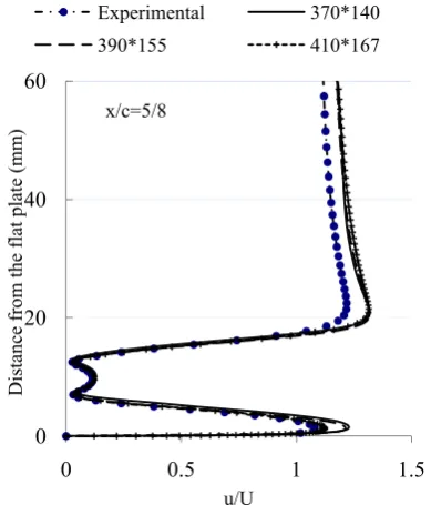
from the flat plate, inside the turbulent boundary layer of the flat plate where Re 1.63E 06. The average velocity profile at downstream to the rod is measured by hotwire, [23]. The comparison between the solution of the present code and measurements at a distance of is presented in Figure 5. x is the distance from the rear stagnation point and c is the length of the quad. As the figure shows, strong agreement exists between the experimental and numerical solutions. The figure compares solutions for three cases of mesh generations with a stretching factor of s 1.08
(grids 410*167), s 1.1 (grids 390*155), and
s 1.12 (grids 370*140). Optimum agreement at s=1.08 is reached and the meshing strategy accepted being employed throughout the present study.
Figure 5. Comparison of mean velocity profiles with measured data.
Another comparison between the present code and the solution of the Fluent code is made by comparing solutions for the same case as explained above. Results are presented in Figure 6. This figure also shows the estimation of the code for HTC compared with the empirical law for a single flat plate. In both cases the code is in satisfactory agreement with the referenced data.
Figure 6. Comparison between the present program and the Fluent code and empirical law for a flat plate.
40 60 80 100 120
0.4 0.5 0.6 0.7
Surf
ace heat transf
er
coef
icient
Length (cm)
RNG K-e Standard K-e Realizable K-e RSM
0 20 40 60
0 0.5 1 1.5
Dis
tance
from
the
flat plate (m
m
)
u/U
Experimental 370*140
390*155 410*167
x/c=5/8
0 10 20 30 40 50 60 70
1.2 1.4 1.6 1.8 2
Heat Transfer
Co
efficient (W
/m
2.K)
X (m)
8. RESULTS AND DISCUSSION
The process of optimization is initiated by random creation of the first twenty individuals making up for the first generation. Each individual represents a quad shape and its distance from the flat plate is as explained in section 5. For each individual, the meshing strategy is applied, then the flow equations are solved and the variation of the local heat transfer coefficient and skin friction is met.
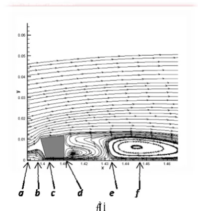
Figure 7 presents the flow solution around a sample quad. Common to all cases of study, as the flow in the boundary layer approaches the quad at point a, a stagnation point forms on the frontal face. As a result, the approaching flow divides into two parts. The first part moves away from the flat plate forming the outer shear layer, which later helps to drive the downstream vortex zone. The lower part of the flow accelerates towards the gap, forming an upstream bubble at point b and a jet at point c. Later, the jet separates from the plate leaving the second bubble on the wall at point e. The jet then joins the external shear flow to drive the circulation zone downstream from the quad. Point f symbolizes the width acting of the circulation zone.
(a)
Figure 7. Flow features around a sample quad at the vicinity of a flat plate, quad a.
Figure 8 shows the variation of the local heat transfer coefficient along a flat plate at similar stages to those discussed in Figure 7. As the figure shows, the upstream bubble causes a small reduction in h at point b. At point c, where the flow accelerates, the boundary layer of the flat plate is washed off and h increases sharply. By
entering the flow into the gap, the boundary layer reshapes and thickens along the way. By thickening the boundary layer, h decreases to a minimum when reaches the second downstream bubble at point e. From point e onwards, h increases again spreading over a wide range of the flat plate length, making a significant contribution to overall heat transfer enhancement, depicted as point f. The existence and contribution of each feature to the heat transfer coefficient is very much dependent on the quad shape.
Such an analysis is made among twenty members of each generation, from which the members of the next generation are decided upon.
Beginning with random creation of the initial population of the first generation, in the range of design variables of Table 1, the algorithm iteratively produces a sequence of new generations until the criterion for halting this sequence, the 80th generation, is encountered. During the process, the selection of parents is based on their fitness; children (or the population of the next generation) are created by making random changes to a single parent (mutation) or by combining the vector entries of a pair of parents (crossover) and then replacing the current population with the next generation. The algorithm selects the most fit to form the next generation. This technique guarantees the algorithm's approach to choosing the best individuals for the last generation.
Figure 8. Typical variation of the local heat transfer coefficient over a flat plate affected by a sample quad
lowest blockage effect. All twenty members of the 80th generation are transcendents of all previous generations and, therefore, form a Pareto front.
(b)
(c)
(d)
Figure 9. Averaged flow field around quads b, c and d of the
pareto front. Flow around quad a, is presented in figure 7.
Figure 10 shows a three-dimensional plot of a variation of h c A for individuals of the 80th generation that are plotted as Pareto front. Each point on this curve represents a quad that is superior to a similar member of the previous generation in that better h or less c and was produced.
Figure 10. Three-dimensional presentation of objective vector components plotted as the Pareto curve.
Figures 7 and 9 demonstrate the flow structure around four selected quads made up of individuals of the last generation (the Pareto front or the 80th generation). Figure 7 shows streamlines around one of these quads (quad a) having the largest cross sectional area, A 112 mm and Figure 9-d provides streamlines for the quad (d) with the least area, A 12.4 mm . Two other figures, 9-b (for quad b with A 50.4 mm ) and 9-c (for quad c with A 23.4 mm ), are selected from points in between the two above mentioned cases of the Pareto curve. As the streamlines show, a stagnation point forms on the frontal area which provides a driving force to run the flow through the gap between the quad and the flat plate. As a result, a jet forms beneath, along with a vortex downstream from the quad. The formation of the vortex is due more to the oncoming flow from the upper side of the obstacle, which dominates all the features of the downstream flow field. Figure 9-b shows that the big vortex has been reduced in size and gradually dies off in Figures 9-c and 9-d, as so does the local heat transfer coefficient, h , in Figure 11. The same occurs by following the reduction of the friction coefficient in Figure 12. Most of the contribution to the enhancement of the heat transfer coefficient, h (reduction in c) is due to the vortex activity which occurs downstream to the obstacle and spreads over a long distance on the flat plate.
More productive discussion can be conducted if Figure 13 is split into two-dimensional plots of
h c, c A, and h A, as are presented in Figures 13 to 15. In each plot, three regions are significant and are named as regions I, II and III. Figure 10 shows the relation between the quads cross sectional areas with a heat transfer
Friction coeffic
ient
0.0035 0.004 0.0045
Heat transfer co
ef. (W
/m2.K)
36 39
42 45
48
Ar
ea
(m
m
2)
Figure 11. Heat Transfer Coefficient plotted along an affected area of the flat plate for obstacles, a, b , c and d.
Figure 12. Skin friction plotted along an affected area of the flat plate for obstacles a, b, c and d
coefficient for twenty individuals of the last generation, i.e. members of the Pareto front. The figure shows that the heat transfer coefficient is directly dependent on the cross sectional area. For quads with small cross sections, a minor change in the quad cross section produces a sharp change in
h , Region I. However, in the Region III the change is smooth.
Figure 13. Pareto curve in 2-D. Presentation of h A for individuals of the last generation.
Figure 14. Pareto curve in 2-D. Presentation of , c A for individuals of the last generation.
In the same way, Figure 14 shows a variation of c
in terms of the quad cross sectional area. The reduction of skin friction due to minor change in quad area is sharp.
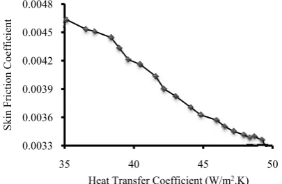
Figure 15 shows that, as the heat transfer coefficient increases, the skin friction coefficient decreases. Amazingly for all 1,600 cases under consideration, an increase in h is simultaneously accompanied by a decrease in c . The phenomenon which is reported and discussed in [4], [5], [6] challenges the Reynolds Analogy between heat and momentum transfer. Region I belongs to small cross sectional obstacles and is
10 20 30 40 50 60
1.37 1.57 1.77 1.97
Heat
Transfer
Coefficient
(W/m
2.K)
X (m)
have=49.81 (W/m2.K) , Area=112 (mm2) , Cf ave=0.0032
have=44.81 (W/m2.K) , Area=50.4 (mm2) , Cf ave=0.0036
have=41.56 (W/m2.K) , Area=23.4 (mm2) , Cf ave=0.004
have=38.35 (W/m2.K) , Area=12.4 (mm2) , Cf ave=0.0044
0 0.002 0.004 0.006 0.008 0.01
1.31 1.51 1.71 1.91
Skin
Friction
Coefficient
x (m)
have=49.81 (W/m2.K) , Area=112 (mm2) , Cf ave=0.0032
have=44.81 (W/m2.K) , Area=50.4 (mm2) , Cf ave=0.0036
have=41.56 (W/m2.K) , Area=23.4 (mm2) , Cf ave=0.004
more suitable for flows moving through limited space heat transfer devices, such as the flow of cooling air through first stage gas turbine blades, in heat exchanger tubes, and other electronic devices, where larger cross sectioned inserts are suitable for boiler walls. However, after a particular insert size increases, i.e. Regions II and III, the sensitivity of
h and c to a variation of is weakened.
Figure 15. Pareto curve in 2-D. Presentation ofh c for individuals of the last generation.
9. CONCLUSION
Using three objective genetic algorithms, the optimization of h , c , and the obstacle cross sectional area is studied for a boundary layer disturbed by an insert. Final results are plotted as a Pareto curve which demonstrates that:
1) Improvement of heat transfer is sharply dependent on quad shape and its cross sectional area. While keeping the quad cross sectional area to a minimum, the genetic algorithm generates the most suitable shapes to maximize heat transfer. In direct relationship, the heat transfer increases as the cross sectional area increases.
2) The insert in the turbulent boundary layer is a cause of the reduction in average skin friction over the affected area of the flat plate; the reduction is a function that increases the cross sectional area. 3) The vortex zone, which is formed while flow moving downstream the obstacle, plays a major
role in enhancement by widening the exited area over the flat plate. As the vortex extends over a larger area, enhancement simultaneously follows. 4) In all 1,600 cases under consideration, an increase in heat transfer is accompanied by a reduction in skin friction. Figures 11 and 12 show that more enhanced heat transfer curve in figure 11, accompanies with lowest skin friction plotted in figure 12.
10. ACKNOWLEDGMENTS
The authors wish to express their gratitude to the Faculty of Engineering, Ferdowsi University of Mashhad, for its financial support of this research project. In addition, they would like to show appreciation for Dr. Amir Beik Khoshnewis of the Sabzevar University for providing the experimental data from wind tunnel hot wire anemometry setup used for verification of the study's computer code.
11. REFERENCES
1. Perry L. Y., “Surface roughness effects on heat transfer
in micro scale single phase”, Proceedings of the Sixth
International ASME Conference on Nano channels, Micro channels and Mini channels, Darmstadt, Germany, June 23-25, (2008)
2. Suzue Y., Morimoto K., Shikazono N., Suzuki Y. and
Kasagi N., “High performance heat exchanger with
oblique wavy walls”, 13th international Heat Transfer
Conference, Sydney, Australia,13-18 August (2006)
3. Liting Tian, Yaling He, Yubing Tao, Wenquan Tao, A
comparative study on the air-side performance of wavy fin-and-tube heat exchanger with punched delta winglets in staggered and in-line arrangements, International Journal of Thermal Sciences Vol. 48, (2009), 1765–1776.
4. Rathod M.K., Shah Niyati K., Prabhakaran P.,
“Performance evaluation of flat finned tube fin heat exchanger with different fin surfaces”, Applied Thermal Engineering Vol. 27, (2007), 2131–2137.
5. Kahrom M., Farievar S., Haidarie A., “The effect of
square splittered and unsplittered rods in flat plate heat
transfer enhancement”, International Journal of
Engineering, Vol 20, No. 1, (2007), 83-94,
6. Inaoka J., Yamamoto J., Suzuki K., “Dissimilarity
between heat transfer and momentum transfer in a disturbed boundary layer with insertion of a
rod-0.0033 0.0036 0.0039 0.0042 0.0045 0.0048
35 40 45 50
Skin Friction
Coefficient
modeling and numerical simulation”, International Journal of Heat and Fluid Flow, Vol. 20, (1999),
290-301.
7. Teraguchi K., Katoh K., Azuma T., “Dissimilarity
between turbulent momentum and heat transfer by
excitation of transverse vortex”, Journal of The Japan
Society of Mechanical Engineers, Vol. 80, (2005)
8. Kong H., Choi H., Lee J. S., “Dissimilarity between the
velocity and temperature fields in a perturbed turbulent
thermal boundary layer”, Phys. Of Fluids, Volume 13,
No. 5, (2001), 1466.
9. Gosselin L., Gingras M.T., Potvin F.M., “Review of
utilization of genetic algorithms in heat transfer
problems”, International Journal of Heat and Mass
Transfer, Vol. 52, (2009), 2169–2188.
10. MacCormack W., Tutty O.R., Rogers E., Nelson P.A.,
“Stochastic optimization based control of boundary
layer transition”, Control Engineering Practice, Vol.
10, No. 3, (200), pp. 243-260.
11. Leng G.S.B., Ng T.T.H., “Application of genetic
algorithms to conceptual design of a micro-air vehicle”,
Engineering Applications of Artificial Intelligence,
Vol. 15, (2002), 439–445.
12. Tiwari S., Chakraborty D., Biswas G., Panigrahi P.K.,
“Numerical prediction of flow and heat transfer in a channel in the presence of a built-in circular tube with
and without an integral wake splitter”, International
Journal of Heat and Mass Transfer, Vol. 48, (2005),
439–453.
13. Amanifard A., Nariman-Zadeh N., Borji M., Khlkhali
A., A. Habibdoust, “Modeling and Pareto optimization of heat transfer and flow coefficients in micro channels using GMDH type neutral networks and genetic
algorithms”, Journal of Energy Conversion and
Management, Vol. 49, No. 2, (2008), 311-325.
14. Xie G.N., Sunden B., Wang Q.W., “Optimization of
compact heat exchangers by a genetic algorithm”,
Applied Thermal Engineering, Vol. 28, (2008), 895–
906.
15. Gholap A.K., Khan J.A., “Design and multi-objective
optimization of heat exchangers for refrigerators”,
Journal of Applied Energy, Vol. 84, (2007), 1226–
1239.
16. Hilbert R., Jaiga G., Barn R., Thevenin D.,
“Multi-objective shape optimization of a heat exchanger using
parallel genetic algorithms”, Int. J. of Heat and Mass
Transfer, Vol. 49, (2006), 2567-2577.
17. Bagley, J.D "The behavior of adaptive systems which
employ genetic and correlation algorithms",
Dissertation Abstracts International, University of
Michigan, Vol. 28 No.12, (1967).
18. Holland J.H., “Adaptation in Natural and Artificial
Systems”, MIT Press ed., ISBN-13: 9780262581110,
(1992).
19. De Jong, K., “Using genetic algorithms to search
program spaces”, Proceedings of the Second
International Conference on Genetic Algorithms, pp.
210–216. Cambridge, MA:Lawrence Erlbaum. (1987)
20. Goldberg D.E., “Genetic algorithms in search,
optimization and machine learning”, Addison-Wesley,
Reading, (1989).
21. Davidson L., “An Introduction to turbulence models”,
Publication 97/2, Department of Thermo and Fluid Dynamics, Chalmers University of Technology,
(2003).
22. Gatski T.B., Hussaini M.Y., Lumley J.L., “Simulation
and modeling of turbulent flows”, ICASE/LaRc series
in Computational Science and Engineering, ISBN
0-19-510643-1 Oxford University Press, (1996).
23. Kahrom M., Khoshnewis A.B., Bani Hashemi H., “Hot
Wire Anemometry in the Wake of Trapezoidals in the Vicinity of a Falt Plate”, Report No. 40258, Faculty of Engineering, Ferdowsi University of Mashhad, Jan.