International Journal of Engineering
J o u r n a l H o m e p a g e : w w w . i j e . i rModeling and Hybrid Pareto Optimization of Cyclone Separators Using Group
Method of Data Handling (GMDH) and Particle Swarm Optimization (PSO)
M. J. Mahmoodabadi*a, M. Taherkhorsandib, H. Safikhanic
a Department of Mechanical Engineering, Sirjan University of Technology, Sirjan, Iran b Young Researchers Club, Rasht branch, Islamic Azad University, Rasht, Iran
c Department of Mechanical Engineering, Amirkabir University of Technology, Tehran, Iran
P A P E R I N F O
Paper history: Received 05 January 2012
Accepted in revised form 30 August 2012
Keywords:
Two-phase Flow Gas-solid
Particle Swarm Optimization Multi-objective Optimization GMDH
A B S T R A C T
In the present study, a three-step multi-objective optimization algorithm of cyclone separators is utilized for the design objectives. First, the pressure drop (Dp) and collection efficiency (h) in a set of cyclone separators are numerically evaluated. Secondly, two metamodels based on the evolved Group Method of Data Handling (GMDH) type neural networks are regarded to model the Dp and h as the required functions of geometrical characteristics. Finally, a multi-objective (MO) algorithm based on hybrid of Particle Swarm Optimization (PSO), multiple crossover and mutation operator are used for Pareto based optimization of cyclones considering two conflicting objectives Dp and h. By comparing the Pareto results of MOPSO with that of multi-objective genetic algorithms (NSGA II) regarding Pareto based multi-objective optimization of the obtained polynomial meta-models, it is shown that there are some interesting and important relationships as useful optimal design principles involved in the performance of cyclone separators.
doi:10.5829/idosi.ije.2013.26.09c.15
NOMENCLATURE
u velocity Greek Symbols
x position r density
P pressure n viscosity
Ne number of effective turns Subscripts
Vin inlet velocity p particle
VP velocity pressure i,j,k 1,2,3
Y Inlet width t turbulent
X Inlet height
R Reynolds stress tensor Superscripts
D50 Cut-point - mean variables
٭ set of decision variables
Ŧ٭ set of objective functions
1. INTRODUCTION 1
Cyclones are widely used in filtration and separation industry because of their simple setup and low cost maintenance. A number of studies were provided which
*Corresponding Author Email:[email protected] (M. J. Mahmoodabadi)
on cyclones of different height and different vortex finder length and found that like other important dimensions such as body diameter and gas exit tube diameter, the cyclone height and vortex finder length can considerably influence the separation efficiency of the cyclones. Ravi et al. [5] investigated an MO optimization process on cyclone separators by using the NSGA algorithm. They tried to minimize the pressure drop and maximize the collection efficiency in cyclone separators. They did not use CFD in their optimization procedure and used analytical function for pressure drop and collection efficiency. Rongbiao et al. [6] suggested that the flow rate has a strong influence on the collection efficiency and the reduction in cone size results in higher collection efficiency without significant increase of pressure drop. Shalaby et al. [7] used Large Eddy Simulation (LES) for CFD modeling of gas-solid flow in cyclones and they obtained good compatibility with experimental results. Safikhani et al. [8] obtained detailed flow information by CFD simulation for three standard cyclone separators with different geometries. They discussed the effects of different geometrical parameters on the pressure drop and collection efficiency. Safikhani et al. [9] investigated an MO optimization algorithm on cyclones using genetic algorithms. They finally determined 5 optimum cyclones which had minimum pressure drop and maximum collection efficiency.
Both pressure drop and collection efficiency in cyclones are important objective functions which must be optimized simultaneously in such a real world complex multi-objective optimization problem. These objective functions are either obtained from experiments or computed using very timely and high-cost Computational Fluid Dynamic (CFD) approaches, which cannot be used in an iterative optimization task unless a simple but effective meta-model is constructed over the response surface from the numerical or experimental data. Therefore, in the present study, modeling and optimization of the parameters are investigated by using Grouped Method of Data Handling (GMDH) type neural networks and Multi-Objective Particle Swarm Optimization method (MOPSO) in order to minimize the pressure drop and maximize the collection efficiency.
System identification and modeling of complex processes using input-output data have always attracted many research efforts. In fact, system identification techniques are applied in many fields in order to model and predict the behavior of unknown and/or very complex systems based on given input-output data [10]. In this way, soft-computing methods [11] which concern computation in an imprecise environment, have gained significant attention. The main components of the soft computing, namely, fuzzy logic, neural network, and evolutionary algorithms have shown great ability in solving complex non-linear system
identification and control problems. Many research efforts have been expended to make use of evolutionary methods as effective tools for system identification [12]. Among these methodologies, Group Method of Data Handling (GMDH) algorithm is a self-organizing approach by which models of growing complexity are generated based on the evaluation of their performances on a set of multi-input-single-output data pairs (Xi, Yi)
(i=1, 2, …, M). The GMDH was first developed by Ivakhnenko [13] as a multivariate analysis method for modeling and identification of complex systems which can be used to model complex systems without having specific knowledge of the systems. The main idea of GMDH is to build an analytical function in a feed forward network based on a quadratic node transfer function [14] whose coefficients are obtained by using the regression technique. In recent years, however, the use of such self-organizing networks leads to successful application of the GMDH-type algorithm in a broad range of areas in engineering, science, and economics.
Particle Swarm Optimization (PSO), first introduced by Kennedy et al. [15], is one of the modern heuristic algorithms. It was developed through simulation of a simplified social system, and has been found to be robust in solving continuous nonlinear optimization problems [15-16]. The PSO technique can generate a high-quality solution within short calculation time and stable convergence characteristic as compared with other stochastic methods [17-18]. In this paper, for increasing the convergence of the population and to escape the local minima, PSO is merged with multiple crossover and mutation operator. Furthermore, over the last decade, the multi-objective PSO has been utilized to solve various types of multi-objective engineering optimization problems [19-21].
In the present study, firstly, the pressure drop (Dp) and the collection efficiency (η) in a set of cyclones are numerically investigated by using CFD techniques. Next, GMDH type neural networks are used to obtain polynomial models for the effects of geometrical parameters of the cyclones on both Dp and η. Finally, the obtained simple polynomial models are used in a Pareto based MOPSO to find the best possible combinations of Dp and η, known as the Pareto front. The Pareto results of MOPSO are also compared with that of multi-objective genetic algorithms (NSGAII).
2. THE CFD SIMULATION AND VALIDATION OF THE RESULTS
velocity coupling. Turbulence fluctuations are simulated by using Reynolds Stress Transport Model (RSTM) due to its accuracy [23], and velocity fluctuations are simulated by using the discrete random walk (DRW). The Lagrangian method is used for tracking of the particles in the simulations; and grid refinement tests are conducted in order to make sure that the solutions do not dependent on the grid. Collection efficiency statistics are obtained by releasing a specific number of particles at the inlet of the cyclones and by monitoring the number escaping through the underflow. The range of particles size is 0.1-10 μm of a material whose density is equal to 2500 kg/m3. The computation continues until the solutions converge into a total residue of less than 0.0001.
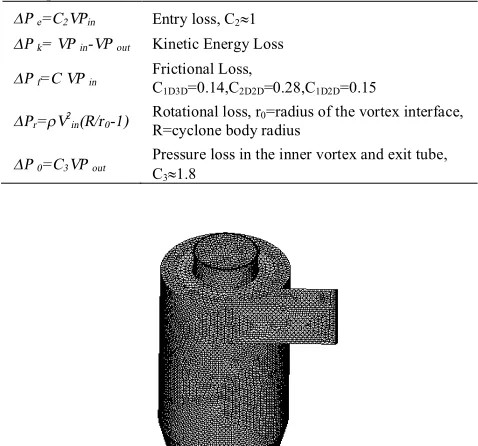
To test for grid independency, three grid types with increasing grid density are studied. The computational results of 3 grid types are compared in Table 1. It was observed that the maximum difference among the results is less than 4%, so that the grid template 186,222 is used for all computations in the present study. Figure 1 shows the details of the computational grid for the cyclones.
2. 2. The Deinition of the Objective Functions The pressure drop and collection efficiency in cyclones are important objective functions which have to be optimized simultaneously. The collection efficiency statistics are obtained by releasing a specified number of particles at the inlet of the cyclones and by monitoring the number escaping through the underflow. The first theory for collection efficiency in conventional cyclones was developed by Shepherd et al. [24]. It is based on the assumption of a plug flow. In order to calculate the efficiency, first the particle size with 50% collection efficiency (Dp50%) needs to be determined according to the following equation:
p in e
P NV
Y D
r p
m
2 9 %
50 = (1)
The collection efficiency for any other particle size (DPj) can then be determined by:
2 % 50
) ( 1
1
Pj p
D D + = h
(2)
Many empirical models have been proposed for the pressure drop in the conventional cyclones [24-27]. In Wang’s model, the total pressure loss in the cyclone is obtained by summing up the five pressure drop components as follows:
DP total=DP e+DP k+DP f+DP r+DPo (3)
where, the components of Equation (3) are explained in Table 2.
2. 3. Deinition of the Design Variables The design variables in the present paper are: the dimensionless length of vortex finder (S/D), dimensionless diameter of vortex finder (De/D), dimensionless length of upside
cyclone (Lup/D) and dimensionless length of downside
cyclone (LDown/D). The design variables and their range
of variations are shown in Figure 2 and Table 3, respectively. The different design variables are selected by dividing (S/D), (De/D), (Dup/D), and (DDown/D) into 3
equal parts. By changing the geometrical independent parameters according to Table 3, various designs will be generated and evaluated by CFD. Consequently, some meta-models can be optimally constructed by using the GMDH type neural networks, which will be further used for the multi-objective Pareto based design of such cyclones.
TABLE 1. The comparison of the dimensionless pressure drop and the collection efficiency for 3 different grid numbers.
Total No. of Cells Dp /0.5v2 η (%)
186,222 10.98 53.07
202,318 11.02 51.42
284,756 11.13 53.12
Max Diff (%) 1.348 3.200
TABLE 2. The components of Wang’s pressure drop theory.
Component Definition
DP e=C2VPin Entry loss, C2»1
DP k= VP in-VP out Kinetic Energy Loss
DP f= C VP in Frictional Loss, C1D3D=0.14,C2D2D=0.28,C1D2D=0.15
DPr=rV2in(R/r0-1) Rotational loss, r0=radius of the vortex interface, R=cyclone body radius
DP 0=C3VP out Pressure loss in the inner vortex and exit tube, C3»1.8
Figure 2. Design variables for the cyclone-optimization problems
Figure 3. The comparison of CFD prediction and experimental data of Konig [28] for pressure drop.
TABLE 3. Design variables and their range of variations
Design Variable From To
S/D 0.900 1.725
De /D 0.125 0.600
Lup /D 0.875 2.775
LDown /D 0.875 2.775
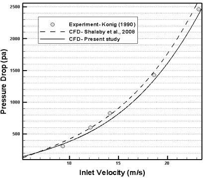
2. 4. Validation of the CFD Results To attain the confidence about the simulation, it is necessary to compare the simulation result with the available data. The comparison of CFD prediction and experimental data of Konig [28] for the pressure drop is shown in Figure 3. As seen, our numerical procedure predicts the pressure drop with the acceptable deviation from the experimental data of Konig [28] and CFD simulations of Shalaby et al. [7], but with increasing the flow rate differences of numerical prediction and experimental
data. This numerical error could contribute and cause the increase of flow complexity in high flow rates.
The comparison of CFD prediction and experimental data of Konig [28] for collection efficiency is shown in Figure 4. It is obvious that our numerical simulations can properly adapt with the pattern of experimental efficiency curve.
Tangential and axial velocities are important factors for the particle collection in the cyclones. Figures 5 and 6 compare the tangential and axial velocity of CFD prediction and experimental data. As seen, the CFD curves of the present study agree well with the experimental data of Fraser et al. [29] and the CFD simulations of Shalaby et al. [7]. Samples of numerical results obtained by using CFD are shown in Table 4; moreover, the velocity vector and pressure contour in one of these CFD simulations are shown in Figure 7.
Figure 4. The comparison of CFD prediction and experimental data of Konig [28] for collection efficiency.
Figure 6. The comparison between the axial velocity of CFD prediction and experimental data.
Figure 7. The velocity vector and pressure contour in the CFD simulations.
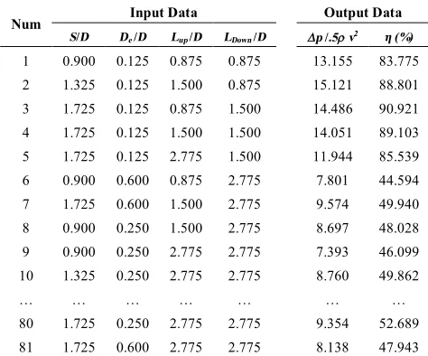
TABLE 4. Samples of numerical results obtained by using
CFD.
Num Input Data Output Data
S/D De /D Lup /D LDown /D Dp /.5r v2 η (%) 1 0.900 0.125 0.875 0.875 13.155 83.775 2 1.325 0.125 1.500 0.875 15.121 88.801 3 1.725 0.125 0.875 1.500 14.486 90.921 4 1.725 0.125 1.500 1.500 14.051 89.103 5 1.725 0.125 2.775 1.500 11.944 85.539 6 0.900 0.600 0.875 2.775 7.801 44.594 7 1.725 0.600 1.500 2.775 9.574 49.940 8 0.900 0.250 1.500 2.775 8.697 48.028 9 0.900 0.250 2.775 2.775 7.393 46.099 10 1.325 0.250 2.775 2.775 8.760 49.862
… … … …
80 1.725 0.250 2.775 2.775 9.354 52.689 81 1.725 0.600 2.775 2.775 8.138 47.943
The results obtained in such CFD analysis can now be used to build the response surface of both collection efficiency and pressure drop for those different 81 geometries using GMDH type polynomial neural networks. Such meta-models will, in turn, be used for the Pareto-based multi-objective optimization of the cyclones. A post analysis using CFD is also performed to verify the optimum results by using the meta-modeling approach. Finally, the solutions obtained by the approach of this paper exhibit some important trade-offs among those objective functions which can be simply used by a designer to optimally compromise among the obtained solutions.
3. MODELING OF PRESSURE DROP AND COLLECTION EFFICIENCY USING GMDH TYPE NEURAL NETWORKS
By means of the GMDH algorithm, a model can be represented as a set of neurons in which different pairs of them in each layer are connected through a quadratic polynomial and thus produce new neurons in the next layer. Such representation can be used in modeling to map inputs to outputs. The formal definition of the identification problem is to find a function fˆ that can be approximately used instead of actual onef in order to predict output yˆ for a given input vector
) ,..., 3 , 2 , 1
(x x x xn
X= as close as possible to its actual output y. Therefore, given M observations of multi-input-single-output data pairs so that
) ,..., 3 , 2 , 1 (
in x i x i x i x f i
y = (i= 1, 2… M) (4)
It is now possible to train a GMDH-type neural network to predict the output values
i
yˆ for any given input vector ( , , ,..., )
3 2
1 i i in i x x x x
X= , that is
) ,..., 3 , 2 , 1 ( ˆ ˆ
in x i x i x i x f i
y = (i= 1, 2… M) (5)
The problem is now to determine a GMDH-type neural network so that the square of difference between the actual output and the predicted one is minimized, that is:
min 2 ] ) ,..., 3 , 2 , 1 ( ˆ 1
[ - ®
å
= i
y in x i x i x i x f M
i
(6)
General connection between input and output variables can be expressed by a complicated discrete form of Volterra functional series in the following form:
...
1 1 1 1 1
1
0 å
= å
= +
å =
å =
å = +
+ å = +
= n
i n
j
n
i n
j k
x j x n
k i
x ijk a j
x i x ij a i
x n
i i
a a
which is known as the Kolmogorov-Gabor polynomial [14]. This full form of mathematical description can be represented by a system of partial quadratic polynomials consisting of only two variables (neurons) in the following form: 2 5 2 4 3 2 1 0 ) , (
ˆ G xi xj a a xi a xj a xixj a xi a xj
y= = + + + + + (8)
There are two main concepts involved within GMDH-type neural networks design, namely, the parametric and the structural identification problems. In this way, some works by Jamali et al. [30] present a hybrid GA and singular value decomposition (SVD) method to optimally design such polynomial neural networks. The methodology in these references has been successfully used in this paper to obtain the polynomial models of Dp and η. The obtained GMDH-type polynomial models have shown to have quite suitable prediction ability of unforeseen data pairs during the training process. This will be presented in the following sections.
The input–output data pairs used in such modeling involve two different data tables obtained from CFD simulation discussed in Section 2. Both tables consist of four variables as inputs, namely (S/D), (De/D), (Lup/D)
and (LDown/D) and outputs which are Dp and η. The
tables consist of a total of 81 patterns, which have been obtained from the numerical solutions to train and test such GMDH type neural networks. However, in order to demonstrate the prediction ability of the evolved GMDH type neural networks, the data in both input–
output data tables have been divided into two different sets, namely, training and testing sets. The training set, which consists of 61 out of the 81 input–output data pairs for Dp and η, is used for training the neural network models using the method presented in Section 2. The testing set, which consists of 20 unforeseen input–output data samples for Dp and η during the training process, is merely used for testing to show the prediction ability of such evolved GMDH type neural network models. The GMDH type neural networks are now used for such input–output data to find the polynomial models of Dp and η with respect to their effective input parameters. In order to genetically design such GMDH type neural networks described in the previous section, a population of 10 individuals with a crossover probability (Pc) of 0.7 and mutation probability (Pm) 0.07 has been used in the 500 generations for Dp and η. The corresponding polynomial representation for dimensionless pressure drop is as follows: ) D L ).( D D ( 55 . ) D L ( .41 ) D D ( 68 . 13 ) D L ( 22 . ) D D ( 69 . 16 20 . 5 1 Y up e 2 up 2 e up e 1 + -+ + -= (9.a) ) D L ( ). D S ( 41 . ) D L ( 81 . ) D S ( 71 . 2 -) D L ( 99 . 3 ) D S ( 92 . 10 52 . 6 Y Down 2 Down 2 Down 2 -+ -+ = (9.b) ) D L ).( D L ( 15 . ) D L ( 81 . ) D L ( 0.41 -) D L ( 80 . 4 ) D L ( 14 . 10 . 7 1 Y Down up 2 Down 2 up Down up 3 + + -+ = (9.c) ) .( ) ( 52 . 1 ) ( 68 . 13 ) ( 71 . 2 ) ( 72 . 13 ) ( 70 . 10 04 . 5 2 2 4 D D D S D D D S D D D S Y e e e -+ -+ = -(9.d) 2 1 2 2 2 1 2 1 5 Y . Y 0.0908 Y 0040 . 0 Y .0037 0 Y 090 . 0 Y 082 . 0 939 . 0 Y + + + -= (9.e) 4 3 2 4 2 3 4 3 6 Y Y 908 0 . 0 Y 0039 . 0 Y 0038 . 0 Y 0876 . 0 Y 0.0847 -934 . 0 Y + + + -= (9.f) 6 5 2 6 2 5 6 5 2 Y Y 368 . 1 Y 685 . 0 Y .682 0 Y 473 . 0 Y 20 5 . 0 0.0308 v 2 1 P -+ + + + = r D (9.g)
Similarly, the corresponding polynomial representation of the model for the collection efficiency is in the following form:
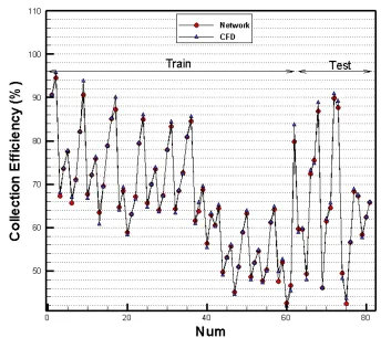
The appropriate behavior of such GMDH type neural network model for the pressure drop is also depicted in Figure 8 for the training and testing data. Such behavior has also been shown for the training and testing data of efficiency in Figure 9. It is evident that the evolved GMDH type neural network in terms of simple polynomial equations successfully model and predict the outputs of the testing data that have not been used during the training process. To determine the accuracy of GMDH modeling, we also use a criterion, namely, Root Mean Square Error (RMSE) which demonstrates the difference between CFD data and GMDH predicted data and can be calculated as follows:
2 1 2
( - )
=
å
fC FD fG M D HR M S E
N (11)
where N is the pattern number and f is Δp or η. The comparison of RMSE for the training and testing data of the objective functions are shown in Table 5. As seen, the GMDH-type neural network predicts the objective functions with the acceptable deviation from CFD data. It should be noted that these polynomials are valid just for the design variables in the range of the present case study (Table 3). The models obtained in this section can now be utilized in the Pareto of the multi-objective optimization algorithm of the cyclone separators considering both the pressure drop and efficiency as the conflicting objectives. Such study may unveil some interesting and important optimal design principles that would not have been obtained without the use of a multi-objective optimization approach.
4. THE PARTICLE SWARM OPTIMIZATION HYBRIDIZED WITH MULTIPLE CROSSOVER AND MUTATION OPERATOR
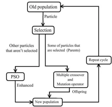
To overcome complexity and dimensionality of real-world problems, it is needed to improve the efficiency and accuracy of PSO. Therefore, to improve the performance of PSO in this paper, it is combined with the multiple crossover and mutation operator to update the particles’ position. In this method, the multiple crossovers are developed to modify the converging process; and also the mutation operator is used to leap from any possible local optima. In the following, the concepts of the PSO, multiple crossover and mutation operator are introduced and in the next section, the hybrid of these operators is described.
4. 1. The Concept of Particle Swarm Optimization
Kennedy et al. [15] originally proposed the PSO algorithm for optimization. PSO is a population-based search algorithm based on the simulation of the social behavior of birds within a flock. Although originally adopted for balancing weights in neural networks [31],
PSO soon became a very popular global optimizer, mainly in problems in which the decision variables are real numbers [32-33].
TABLE 5. The comparison of RMSE for objective functions.
Objective Function Train Test
Δp 0.08132 0.0731
η 1.03701 1.0011
Figure 8. The behavior of GMDH type neural network model for the pressure drop of the training and testing data.
Figure 9. The behavior of GMDH type neural network model for the efficiency of the training and testing data.
changed by adding a velocity vi(t) ®
to the current position, i.e.:
) 1 ( ) ( ) 1
( + =® +® +
®
t v t x t
xi i i (12)
The velocity vector reflects the socially exchanged information and, in general, is defined as the following formula:
)) ( (
) ( ) 1
(t Wv t Cr x x t
vi i globalbest i
® ®
® ®
-+
=
+ (13)
where rÎ[0,1] is a random value, C is the social learning factor and represents the attraction that a particle has toward the success of its neighbors, W is the inertia weight which is employed to control the impact of the previous history of velocities on the current velocity of a given particle. xglobalbest
®
is the position of the best particle of the entire swarm [34].
4. 2. The Concept of the Multiple Crossovers and Mutation Operator
4. 2. 1. The Multiple Crossovers Unlike the traditional crossover using only two chromosomes, a crossover formula that contains three parent chromosomes is used in this study. We assume that chromosome x®i(t) is randomly selected from the population. Also, let r Î [0,1] be a random number. If r< pCrossover, then the following multiple crossovers are performed to generate a new chromosome,
)) ( ) ( ) ( 2 ( ) ( )
(t x t x t x 1 t x 2 t
xi i i i i
® -®
-® ®
®
-+
= s (14)
where
s
Î
[
0
,
1
]
is a random value. If r³ pCrossover, the crossover operation is not performed.4. 2. 2. The Mutation Operator The mutation operator provides a possible mutation on some chosen chromosomes x®i(t). Also, let JÎ[0,1] be a random number. If J<pMutation, then the following mutation operator is performed to generate a new chromosome,
k
x´
+ =®
®
) ( ) (t x t
xi i (15)
where xÎ[0,1] is a random value and
k
is a positive constant. If J³pMutation, no crossover operation is performed.Figure 10. The flow chart of the hybrid of PSO, multiple crossovers and mutation operator.
4. 3. The Hybrid of PSO, Multiple Crossover and Mutation Operator The flow chart of the hybrid of PSO, multiple crossover and mutation operator is shown in Figure 10. In the start of each iteration, two random numbers between zero and one are considered (r and
J
) for each particle. If r<pCrossover orMutation p <
J , then the multiple crossovers or the mutation operator will be performed respectively. However, if r³pCrossover and J³ pMutation , this particle will be enhanced by PSO.
the specialized literature. The problems are of the following type :
Minimize ( ): [ ( ), ( ),..., ( )]
2 1
® ® ® ® ®
= f x f x f x x
f k (16)
Subject to:
m i
x
gi( )£0 =1,2,...,
®
(17)
p i
x
hi( )=0 =1,2,...,
®
(18)
where T
n x x x
x=[ 1, 2,..., ]
®
is the vector of decision
variables, f Rn R i k
i: ® , =1,..., are the objective
functions and g h Rn R i m j p
j
i, : ® , =1,..., , =1,..., the constraint functions of the problem. To describe the concept of optimality, we will introduce next a few definitions, as follows:
· Dominance: Given two vectors ®x,®yÎRk we say
that ®x£®y if xi yi ® ®
£ for
i
=
1
,...,
n
and that®x
dominates ®y (denoted by ®xp®y) if ® ®
£
y
x
and® ®
¹y
x .
· Non-Dominance: We say that a vector of decision variables ®xÎcÌRn is non-dominated with respect
toc, if there does not exist another ®x¢Îc such that
) ( ) (® ® ®
®
¢ f x
x
f p .
· Pareto-optimal: We say that a vector of decision variables x®*ÎFÌRn (F is the feasible region) is Pareto-optimal if it is non-dominated with respect to F.
· Pareto Optimal Set: The Pareto-optimal Set p*is
defined by: p*={®xÎF|®xispareto-optimal}. · Pareto Front: The Pareto FrontpF*is defined by:
} | ) (
{® ® ® *
*= f x ÎR xÎp
pF k .
Thus, the Pareto optimal set of the set F of all the decision variable vectors are determined in such a way that satisfies Equations (16) and (17). However, note that all the Pareto optimal set is not normally desirable or achievable in practice (e.g., it may not be desirable to have different solutions that map to the same values in the objective function space). In order to apply the PSO strategy for solving multi-objective optimization problems, the original scheme obviously has to be modified. The solution set of a problem with multiple objectives does not consist of a single solution (in the global optimization). Instead, in multi-objective optimization, we aim to find a set of different solutions (the so-called Pareto optimal set). When solving
single-objective optimization problems, xglobal best
®
is used as a leader to update particles’ position. However, in the case of multi-objective optimization problems, each particle might have a set of different leaders from which just one can be selected in order to update its position. Such a set of leaders is usually stored in a different place from the swarm, that we will call "external archive": This is a repository in which the non-dominated solutions found so far are stored. However, if all non-dominated solutions are retained in the archive, then the size of the archive increases very quickly. This is an important issue because the archive has to be updated at each generation. Thus, this update may become very expensive, computationally, if the size of the archive grows too much. Therefore, the archive tends to be bounded, which makes necessary the use of an additional criterion to decide which non-dominated solutions to retain.
In this paper, it is an adopted ε-elimination technique to prune the archive. In this approach, the entire particles in the archive have a neighborhood radius that is equal to ε and if a particle has a distance fewer than ε to another, the particle will be eliminated in the objective function space. Here, the following equation is used to determine ε:
generation maximum
t ´
= s
e (19)
where t is the time step and
s
is a positive constant. The contents of the external archive are also reported as the final output of the algorithm. In this paper, we describe a leader selection technique that is based on the density measures. For this propose, a neighborhood radius for each particle in archive is defined. Then, the number of these particles’ neighborhoods is calculated in the objective function space. The particle that has fewer number of neighborhood is preferred as leader.5.MULTI-OBJECTIVE OPTIMIZATION OF CYCLONE SEPARATORS USING THE HYBRID OF PSO, MULTIPLE CROSSOVERS AND MUTATION OPERATOR
In order to investigate the optimal performance of the cyclone separators in different geometrical parameters, the polynomial neural network models obtained in Section 3 are now deployed in a multi-objective optimization procedure. In the MO hybrid algorithm, the inertia weight W is nonlinearly decreased over time by the following equation:
5 . 0 2
1
1 ( ) ( )
generation maximum
t W
W W
W= - - ´ (20)
2
) (
) (
generation maximum
t C
C C
C= i- i- f ´ (21)
where W1=0.75,W2=0.25, Ci=0, and Cf =2.5. The related variables used in the multiple crossovers and mutation operator are: pCrossover =0.7, pMutation =0.2,
and k=0.05. Furthermore, the term vi(t)
®
is limited to the range [-1,+1] and if the velocity violates this range, a random number from [0,1] is multiplied by it. Based on the observation of the movement of the Pareto front, the population size is set to 100 and the maximum iteration is also set to 100. The two conflicting objectives in this study are Dp and η which have to be simultaneously optimized with respect to the design variables (S /D), (De/D), (Lup/D) and (LDown/D). The
multi-objective optimization problem can be formulated in the following form:
Maximizethe Collection Efficiency (η) = ( , , , ) 1
D L D L D D D
S
f e up Down
Minimize the Pressure Drop (Dp) = ( , , , )
2 D
L D L D D D S
f e up Down
Subject to 0.9 1.725
1= £ £
D S x
(22)
6 . 0 125
.
0 £ 2= £
D D
x e
775 . 2 875
.
0 £ 3= D £
L
x up
775 . 2 875
.
0 £ 4= £
D L
x Down
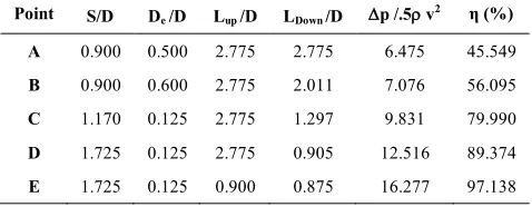
The variable in Equation (22) is the maximum or minimum value having a standard cyclone. Figure 11 depicts the obtained non-dominated optimum design points as a Pareto front of those two objective functions. There are five optimum design points, namely, A, B, C,
D and E whose corresponding design variables and objective functions are shown in Table 6. These points clearly demonstrate tradeoffs in objective functions, pressure drop and collection efficiency, from which an appropriate design can be compromisingly chosen. It is clear from Figure 11 that all the optimum design points in the Pareto front are non-dominated and could be chosen by a designer as an optimum cyclone separator. Evidently, choosing a better value for any objective function in the Pareto front would cause a worse value for another objective. The corresponding decision variables of the Pareto front shown in Figure 11 are the best possible design points so that if any other set of decision variables is chosen, the corresponding values of the pair of objectives will locate a point inferior to this Pareto front. In fact, such inferior area in the space of the two objectives is bottom/right side of Figure 11. In Figure 11, the design points A and E stand for the
best pressure drop and the best collection efficiency, respectively. Moreover, the other optimum design points, B and D can be simply recognized from Figure 11. The design point, B exhibits important optimal design concepts. In fact, optimum design point B
obtained in this paper exhibits an increase in the pressure drop (about 6.1%) in comparison with that of point A, while its efficiency improves about 20.3 % in comparison with that of A. Similarly, optimum design point D exhibits a decrease in efficiency (about 14.5%) in comparison with that of point E, while its pressure drop improves about 38 % in comparison with that of E. Table 6 shows the maximum and minimum collection efficiency obtained from the minimum and maximum of (De/D), (Lup/D), and (LDown/D). These results are
compatible with those of Zhu et al. [4] and Lim et al. [36]. It means that a decrease in De/D, Lup/D, and
LDown/D leads to an increase in the collection efficiency
and pressure drop. It is now desired to find a trade-off optimum design point compromising both objective functions. This can be achieved by the method employed in this paper, namely, the mapping method (normalization method).
TABLE 6. The values of objective functions and their associated design variables of the optimum points.
Point S/D De /D Lup /D LDown /D Dp /.5r v2 η (%)
A 0.900 0.500 2.775 2.775 6.475 45.549
B 0.900 0.600 2.775 2.011 7.076 56.095
C 1.170 0.125 2.775 1.297 9.831 79.990
D 1.725 0.125 2.775 0.905 12.516 89.374
E 1.725 0.125 0.900 0.875 16.277 97.138
In this method, the values of objective functions of all non-dominated points are mapped into interval 0 and 1. Using the sum of these values for each non-dominated point, the trade-off point simply is one having the minimum sum of those values. Consequently, optimum design point C is the trade-off point obtained from the mapping method.
The Pareto front obtained from the proposed method (Figure 11) has been superimposed with the Pareto front of multi-objective genetic algorithm, NSGA II [37], and the corresponding CFD simulation results in Figure 12. It can be clearly seen from this figure that the proposed Pareto front lies on the best possible combination of the objective values of CFD data and achieves better objective functions than NSGA II for the present case study (cyclone separators), which demonstrate the effectiveness of this investigation in obtaining the optimal Pareto front.
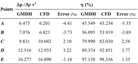
In a post numerical study, the design points of the obtained Pareto front have been re-evaluated by CFD. It should be noted that the optimum design points of the MOPSO method are not included in the training and testing sets using GMDH-type neural network which makes such re-evaluation sensible. The results of such CFD analysis re-evaluations have been compared with those of numerical results using GMDH polynomials in Table 7. As seen, the optimum GMDH data agree well with the CFD results. Shi et al. [38] found that for the optimization problems with a large number of parameters and objective functions, a limited number of CFD evaluations are not sufficient. However, such a good agreement between network and CFD re-evaluation data in this paper is due to the large number of CFD simulations.
In fact, we have studied a problem with two objective functions and four design variables with 81 different designs which are sufficient to cover the domain of different designs.
Figure 12. The comparison among the Pareto front obtained from the proposed method, NSGA II, and the corresponding CFD simulation results.
TABLE 7. Re-evaluation of the obtained optimal Pareto front using CFD.
Points Dp /.5r v
2 h (%)
GMDH CFD Error (%) GMDH CFD Error (%)
A 6.475 6.201 -4.41 45.549 43.234 -5.35
B 7.076 6.821 -3.73 56.095 53.919 -3.89
C 9.831 10.042 2.10 79.990 82.030 2.56
D 12.516 12.933 3.22 89.374 92.851 3.77
E 16.277 16.090 -1.16 97.138 98.336 1.35
6. CONCLUSION
Two different polynomial relations for the collection efficiency and pressure drop have been found by evolved GS-GMDH type neural networks using some experimentally validated CFD simulations for input–
output data of the cyclone separators. The derived polynomial models have been used in the MOPSO optimization process; therefore, some interesting informative optimum design aspects have been revealed for the cyclones. The Pareto front of the hybrid of MOPSO and NSGA II methods have been compared. It was illustrated that MOPSO Pareto front lies on the best possible combination of the objective values of CFD data and achieves better objective functions than NSGA II for the present case study.
[1-38]
7. REFERENCES
1. Stairmand, C. J., "The design and performance of cyclone separators", Transactions of Institute of Chemical Engineers, Vol. 29, No., (1951), 356-383.
2. Dirgo, J. and Leith, D., "Performance of theoretically optimised cyclones", Filtration & Separation, Vol. 22, No. 2, (1985), 119-125.
3. Cheremisinoff, P. N., "Air pollution control and design for industry", CRC Press, (1993).
4. Zhu, Y. and Lee, K., "Experimental study on small cyclones operating at high flowrates", Journal of Aerosol Science, Vol. 30, No. 10, (1999), 1303-1315.
5. Ravi, G., Gupta, S. K. and Ray, M., "Multiobjective optimization of cyclone separators using genetic algorithm", Industrial & Engineering Chemistry Research, Vol. 39, No. 11, (2000), 4272-4286.
6. Xiang, R., Park, S. and Lee, K., "Effects of cone dimension on cyclone performance", Journal of Aerosol Science, Vol. 32, No. 4, (2001), 549-561.
7. Shalaby, H., Wozniak, K. and Wozniak, G., "Numerical calculation of particle-laden cyclone separator flow using les", Engineering Applications of Computational Fluid Mechanics, Vol. 2, No. 4, (2008), 382-392.
9. Safikhani, H., Hajiloo, A. and Ranjbar, M., "Modeling and multi-objective optimization of cyclone separators using cfd and genetic algorithms", Computers & Chemical Engineering, Vol. 35, No. 6, (2011), 1064-1071.
10. Åström, K. and Eykhoff, P., "System identification—a survey", Automatica, Vol. 7, No. 2, (1971), 123-162.
11. Sanchez, E., Shibata, T. and Zadeh, L. A., "Genetic algorithms and fuzzy logic systems: Soft computing perspectives", World Scientific, Vol. 7, (1997).
12. Kristinsson, K. and Dumont, G. A., "System identification and control using genetic algorithms", Systems, Man and Cybernetics, IEEE Transactions on, Vol. 22, No. 5, (1992), 1033-1046.
13. Ivakhnenko, A., "Polynomial theory of complex systems", Systems, Man and Cybernetics, IEEE Transactions on, Vol., No. 4, (1971), 364-378.
14. Farlow, S. J., "Self-organizing methods in modeling: Gmdh type algorithms", CrC Press, Vol. 54, (1984).
15. Kennedy, J., "Particle swarm optimization, in Encyclopedia of machine learning", , Springer, (2010), 760-766.
16. Angeline, P. J., "Using selection to improve particle swarm optimization", in Evolutionary Computation Proceedings, 1998. IEEE World Congress on Computational Intelligence., The 1998 IEEE International Conference on, IEEE. (1998), 84-89. 17. Eberhart, R. C. and Shi, Y., "Comparison between genetic
algorithms and particle swarm optimization", in Evolutionary Programming VII, Springer. (1998), 611-616.
18. Yoshida, H., Kawata, K., Fukuyama, Y., Takayama, S. and Nakanishi, Y., "A particle swarm optimization for reactive power and voltage control considering voltage security assessment", Power Systems, IEEE Transactions on, Vol. 15, No. 4, (2000), 1232-1239.
19. Rahimi-Vahed, A., Mirghorbani, S. and Rabbani, M., "A hybrid multi-objective particle swarm algorithm for a mixed-model assembly line sequencing problem", Engineering Optimization, Vol. 39, No. 8, (2007), 877-898.
20. Janga Reddy, M. and Nagesh Kumar, D., "An efficient multi-objective optimization algorithm based on swarm intelligence for engineering design", Engineering Optimization, Vol. 39, No. 1, (2007), 49-68.
21. Annamdas, K. K. and Rao, S. S., "Multi-objective optimization of engineering systems using game theory and particle swarm optimization", Engineering Optimization, Vol. 41, No. 8, (2009), 737-752.
22. Safikhani, H., Akhavan-Behabadi, M., Shams, M. and Rahimyan, M., "Numerical simulation of flow field in three types of standard cyclone separators", Advanced Powder Technology, Vol. 21, No. 4, (2010), 435-442.
23. Raoufi, A., Shams, M. and Kanani, H., "Cfd analysis of flow field in square cyclones", Powder Technology, Vol. 191, No. 3, (2009), 349-357.
24. Cooper, C. D. and Alley, F. C., "Air pollution control: A design approach", Waveland Press Long Grove, Ill, Vol. 2, (2002). 25. Casal, J. and Martinez-Benet, J. M., "Better way to calculate
cyclone pressure drop", Chemical Engineering, Vol. 90, No. 2, (1983), 99-100.
26. Coker, A., "Understand cyclone design", Chemical Engineering Progress;(United States), Vol. 89, No. 12, (1993).
27. Wang, L., Theoretical study of cyclone design", Texas A&M University, (2004).
28. König, C., "Untersuchungen zum abscheideverhalten von geometrisch ähnlichen zyklonen", (1990).
29. Fraser, S., Abdel-Razek, A. and Abdullah, M., "Computational and experimental investigations in a cyclone dust separator", Proceedings of the Institution of Mechanical Engineers, Part E: Journal of Process Mechanical Engineering, Vol. 211, No. 4, (1997), 247-257.
30. Jamali, A., Nariman-Zadeh, N., Darvizeh, A., Masoumi, A. and Hamrang, S., "Multi-objective evolutionary optimization of polynomial neural networks for modelling and prediction of explosive cutting process", Engineering Applications of Artificial Intelligence, Vol. 22, No. 4, (2009), 676-687. 31. Eberhart, R., Simpson, P. and Dobbins, R., "Computational
intelligence pc tools", Academic Press Professional, Inc., (1996).
32. Engelbrecht, A. P., "Computational intelligence: An introduction", Wiley. com, (2007).
33. Engelbrecht, A. P., "Fundamentals of computational swarm intelligence", Wiley Chichester, Vol. 1, (2005).
34. Chau, K., "Application of a pso-based neural network in analysis of outcomes of construction claims", Automation in Construction, Vol. 16, No. 5, (2007), 642-646.
35. Moore, J. and Chapman, R., "Application of particle swarm to multiobjective optimization", Department of Computer Science and Software Engineering, Auburn University, (1999). 36. Lim, K., Kim, H. and Lee, K., "Characteristics of the collection
efficiency for a cyclone with different vortex finder shapes", Journal of Aerosol Science, Vol. 35, No. 6, (2004), 743-754. 37. Deb, K., Pratap, A., Agarwal, S. and Meyarivan, T., "A fast and
elitist multiobjective genetic algorithm: Nsga-ii", Evolutionary Computation, IEEE Transactions on, Vol. 6, No. 2, (2002), 182-197.
Modeling and Hybrid Pareto Optimization of Cyclone Separators Using Group
Method of Data Handling (GMDH) and Particle Swarm Optimization (PSO)
M. J. Mahmoodabadia, M. Taherkhorsandib, H. Safikhanic
a Department of Mechanical Engineering, Sirjan University of Technology, Sirjan, Iran b Young Researchers Club, Rasht branch, Islamic Azad University, Rasht, Iran
c Department of Mechanical Engineering, Amirkabir University of Technology, Tehran, Iran
P A P E R I N F O
Paper history: Received 05 January 2012
Accepted in revised form 30 August 2012
Keywords:
Two-phase Flow Gas-solid
Particle Swarm Optimization Multi-objective Optimization GMDH
هﺪﯿﮑﭼ
ﻪﻠﺣﺮﻣﻪﺳﯽﻓﺪﻫﺪﻨﭼيزﺎﺳﻪﻨﯿﻬﺑﻢﺘﯾرﻮﮕﻟا ﮏﯾ،ﻖﯿﻘﺤﺗﻦﯾارد هﺪﻨﻨﮐاﺪﺟ ياﺮﺑيا
ﻪﺑنﺪﯿﺳررﻮﻈﻨﻣﻪﺑوﯽﻧﻮﻠﮑﯿﺳيﺎﻫ
فﺪﻫ ﺖﺳاهﺪﺷﻪﺘﻓﺮﮔﺮﻈﻧردﯽﺣاﺮﻃيﺎﻫ
.
رﺎﺸﻓﺖﻓااﺪﺘﺑا Dp
عﻮﻤﺠﻣهدزﺎﺑو h
ﻪﻋﻮﻤﺠﻣﮏﯾرد ي
هﺪﻨﻨﮐاﺪﺟ ي ﯽﻧﻮﻠﮑﯿﺳ
ﯽﻣﻪﺒﺳﺎﺤﻣيدﺪﻋترﻮﺻﻪﺑ دﻮﺷ
.
ﻪﺒﺷسﺎﺳاﺮﺑﺎﺘﻣلﺪﻣود،ﺲﭙﺳ عﻮﻧﯽﺒﺼﻋ
GMDH يزﺎﺳلﺪﻣياﺮﺑ Dp
و h ﻪﺑ
ﯽﮔﮋﯾوﻪﺑﻪﺟﻮﺗﺎﺑوزﺎﯿﻧدرﻮﻣﻊﺑاﻮﺗناﻮﻨﻋ ﺖﺳاهﺪﺷﻪﺘﻓﺮﮔﺮﻈﻧردﯽﺳﺪﻨﻫيﺎﻫ
.
ﻪﯾﺎﭘﺮﺑﯽﻓﺪﻫﺪﻨﭼﻢﺘﯾرﻮﮕﻟاﮏﯾزا ي
ﻪﻨﯿﻬﺑ
نﻮﻠﮑﯿﺳﯽﯾﻮﺗرﺎﭘيزﺎﺳﻪﻨﯿﻬﺑياﺮﺑﺶﻬﺟﺮﮕﻠﻤﻋوﻪﻧﺎﮔﺪﻨﭼمﺎﻏدا،هرذﯽﻌﻤﺠﺗيزﺎﺳ دﺎﻀﺘﻣفﺪﻫﻊﺑﺎﺗودﻪﺑﻪﺟﻮﺗﺎﺑوﺎﻫ
ﺖﺳاهﺪﺷهدﺎﻔﺘﺳا
.
ﻪﻨﯿﻬﺑﺞﯾﺎﺘﻧﻪﺴﯾﺎﻘﻣﺎﺑ زا هﺪﻣآﺖﺳدﻪﺑﺎﺘﻣلﺪﻣودﯽﯾﻮﺗرﺎﭘﻪﻓﺪﻫﺪﻨﭼيزﺎﺳ
MOPSO ﻢﺘﯾرﻮﮕﻟاو
ﻪﻓﺪﻫﺪﻨﭼﮏﯿﺘﻧژ NSGA II
ياﺮﺑﯽﻤﻬﻣﻂﺑاور، هﺪﻨﻨﮐاﺪﺟدﺮﮑﻠﻤﻋردﻪﻨﯿﻬﺑﯽﺣاﺮﻃ
ﺖﺳاهﺪﻣآﺖﺳدﻪﺑﯽﻧﻮﻠﮑﯿﺳيﺎﻫ
.