Optimization of Minimum Quantity Liquid Parameters in Turning for the
Minimization of Cutting Zone Temperature
T. Tamizharasana, J. Kingston Barnabas*b
aPrincipal, TRP Engineering College, Irungalur, Tiruchirappall - 621 105
bDepartment of Mechanical Engineering, Anjalai Ammal Mahalingam Engineering College, Kovilvenni, Tiruvarur District – 614 403
P A P E R I N F O
Paper history: Received 19 July 2011
Received in revised form 16 April 2012 Accepted 17 September 2012
Keywords:
Cutting Zone Temperature Surface Roughness
Taguchi’s Design Of Experiments Particle Swarm Optimization Simulated Annealing Algorithm Differential Evolution
A B S T R A C T
The use of cutting fluid in manufacturing industries has now become more problematic due to environmental pollution and health related problems of employees. The minimization of cutting fluid also leads to the saving of lubricant cost and cleaning time of machine, tool and work-piece. The concept of minimum Quantity Lubrication (MQL) has come in to practice since a decade ago in order to overcome the disadvantages of flood cooling. This experimental investigation deals with the effects of MQL parameters during turning for the minimization of cutting zone temperature by considering surface roughness as constraint. The selected MQL parameters are varied through four levels. The maximum temperature values during machining in all the test conditions as per L16 orthogonal array are recorded. The best levels of selected MQL parameters for the minimization of cutting zone temperature were identified using Taguchi’s Design of Experiments. A validation experiment is conducted with the identified best levels of parameters and the corresponding cutting zone temperature is recorded. This analysis further inter-relates the performances of Particle Swarm Optimization (PSO), Simulated Annealing Algorithm (SAA) and Differential Evolution (DE) for the minimization of cutting zone temperature. The results obtained from DE are comparatively better than that of the results obtained from other techniques.
doi:10.5829/idosi.ije.2012.25.04c.08
1. INTRODUCTION1
In general, dry hard machining generates higher cutting zone temperature, which causes lot of problems such as dimensional deviation, premature failure of cutting tools, surface integrity of the product etc.,. In high speed machining, the conventional flood cooling fails to penetrate in to the chip-tool interface and thus it does not reduce the tool-chip interface temperature which is well described by Paul et al. [1]. The advantages of using the cutting fluids have been questioned lately because of several negative effects such as damaging of soil, creating health related problems to workers, making environmental problems etc., due to mishandling of used cutting fluids. Handling and disposal of cutting fluids should obey the rigid rules of environmental protection which is well stated by Sokovic et al. [2].
* Corresponding Author Email: [email protected] (J. Kingston Barnabas)
The dry machining sometimes less effective when there is a requirement of higher machining efficiency, better surface finish etc.,. In this situation, MQL machining using very small amount of cutting fluids is expected to become a powerful tool.
MQL in machining refers to the use of smaller amount of cutting fluids, typically 100 ml/hr or even less as stated by Diniz et al. [3] which is an alternative to dry or flood cooling methods. Many researchers have suggested that MQL has the potential competitiveness in terms of tool life, surface finish and cutting forces in various manufacturing processes such as turning [4], milling [5] and drilling [6].
Tasdelena et al. [7] carried out an experimental analysis to study the influence of media such as MQL, compressed air and emulsion on tool chip contact length. The results showed that MQL lowers the contact length compared to dry cutting at short and longer engagement times. In the experimental work of Rahman [8], it is proved that MQL technique during machining is a good alternative to dry machining and flood
International Journal of Engineering
cooling. Once again in the experimental analysis of Kamata et al. [9], the use of MQL not only increases the tool life but also the surface finish when compared to wet cutting. The effect of cutting speed and feed rate on machinability aspects were studied and concluded that MQL type of lubrication can successfully replace the flood lubrication while machining.
An experimental investigation was carried out by Davim et al. [10] on machining of brass under different condition of lubricant environments. The investigation on the effects of air-oil mixture application on cutting temperature, cutting forces and flank wear has been studied by Kuan-Ming Li et al. [11]. Effects of minimum quantity lubrication on turning AISI 9310 alloy steel using vegetable based cutting fluid on cutting zone temperature for various process parameters has been studied in the experimental work of Khan et al. [12] for various feed, speed and depth of cut. Gaitondea et al. [13] carried out an experimental work for obtaining optimal machining parameters like quantity of lubricant, cutting speed and feed rate. Dhar et al. [14] carried out an experimental investigation to analyze the effects of machining parameters like cutting velocity, feed rate and depth of cut on cutting temperature, chip reduction coefficient, cutting forces, tool wears, surface finish, and dimensional deviation. From the literature review, it is come to know that there is no systematic research work to determine the optimum values of density of cutting fluid, quantity of lubricant and pressure of air for achieving lower cutting zone temperature. Hence, an attempt has been made in this investigation to analyze the reduction in cutting zone temperature and in the increase of surface roughness by selecting the density of cutting fluid, quantity of lubricant and pressure of air as the process parameters.
In the experimental work of Dhar et al. [15], there is complexity in constructing a long carbide rod to extend the cutting insert to monitor the parasitic emf generated while measuring cutting temperature during machining. Hence, in this investigation, the rise in cutting zone temperature is monitored and measured on on-line basis by 2 mm diameter K–type thermocouple which is brazed in to the holes already drilled on the cutting inserts.
Conventional optimization techniques are used only for local optimal solutions. Consequently, non-traditional optimization techniques are used for global optimization. Liu et al. [16] have done comparative analysis of conventional and non-conventional optimization techniques for CNC turning process. Vijayakumar et al. [17] used Ant Colony system for the optimization of multi-pass turning operations. The optimization problem in turning has been solved by Genetic Algorithms, simulated annealing and particle swarm optimization to obtain more accurate results by Milfelner et al. [18]. Asokan et al. [19] optimized the
surface grinding operations using Particle Swarm Optimization technique. The application of PSO in scheduling of Flexible Manufacturing Systems have been studied by Jerald et al. [20]. Goldberg [21] described the use of Genetic Algorithm optimization technique in machining. Price et al. [22] used Differential Evolution (DE) technique which is an improved version of Genetic Algorithm for faster optimization. So, many optimization techniques were applied for the optimization of parameters of MQL during machining of various materials, but most of the authors had not been considered the more practically used machine component as specimen. In addition to the above, the results of Taguchi’s Design of Experiments, Simulated Annealing Algorithm, Particle Swarm Optimization and Differential Evolution are also compared and correlated as different cases.
According to the literature review, the MQL parameters which affect the cutting zone temperature during machining and surface roughness of finished component are type of coolant oil, mass flow rate of coolant oil and pressure of air. Hence it is decided to vary the above said MQL parameters for analyzing the cutting zone temperature.
In addition, most of the authors [12, 14] kept the pressure of air as constant. But in this study, the pressure of air is varied through four levels in addition to other two parameters such as density of oil and mass flow rate of oil and the effect on cutting zone temperature has been studied.
In the experimental study of Tamizharasan et al. [23], it has been stated that the Simulated Annealing Algorithm converges faster. However, as a new comparison, two emerging techniques such as Particle Swarm Optimization and Differential Evolution have been taken in this study to be compared with Simulated Annealing Algorithm. The objective of present study is to identify the technique which is well suited to optimize the best combination of MQL parameters which gives better performance.
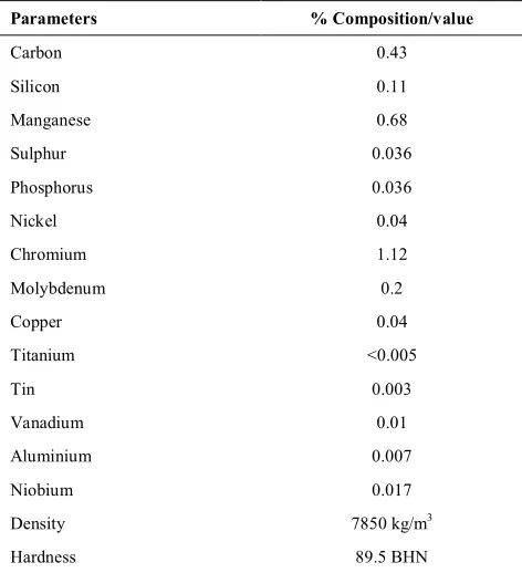
The present study investigates the effect of various parameters of MQL during machining for the minimization of cutting zone temperature while machining ASTM E 415 08 with chemical composition and physical properties were presented in Table. It has wide application such as manufacturing of automobile axle shafts, automobile worm shafts, crank shafts, connecting rods and high tensile bolts & studs.
2. METHODOLOGY USED
TABLE 1. Chemical composition and physical properties of ASTM E 415 08
Parameters % Composition/value
Carbon 0.43
Silicon 0.11
Manganese 0.68
Sulphur 0.036
Phosphorus 0.036
Nickel 0.04
Chromium 1.12
Molybdenum 0.2
Copper 0.04
Titanium <0.005
Tin 0.003
Vanadium 0.01
Aluminium 0.007
Niobium 0.017
Density 7850 kg/m3
Hardness 89.5 BHN
These statistical data are obtained from regression analysis. A validation experiment is conducted with the identified levels of MQL parameters. The non- traditional optimization techniques such as Particle Swarm Optimization, Simulated Annealing Algorithm and Differential Evolution are also used to identify the best values of MQL parameters for the minimization of cutting zone temperature. The details of experiment conducted and analysis carried out is shown as flowchart in Figure 1.
2. 1. Taguchi’s Design of Experiments There are many ways to design a test, but the most frequently used approach is a full factorial experiment. However, for full factorial experiments, there are 2n possible
combinations that must be tested where ‘n’ is number of parameters. Therefore, it is very time-consuming when there are many factors.
In order to reduce the number of experiments to be conducted for the same number of parameters and levels, the Taguchi’s Design of Experiments employs a specially designed orthogonal array. The minimum number of experiments to be conducted is calculated as, [(L – 1) x P] + 1 = [(4-1) × 3]+1=10≈L16
Hence, the Taguchi’s Design of experiments employs L16 orthogonal array to identify the values of
selected parameters for the minimization of cutting zone temperature. An objective function with a constraint is formulated to identify the optimal values of selected
MQL parameters for the minimization of cutting zone temperature.
Since the objective is cutting zone temperature which is to be minimized, lower-the-better category is selected to calculate the S/N ratio. The S/N ratio for cutting zone temperature is calculated as,
2 -1 0
1
- 1 0 lo g y
n å
where, n is the number of serials of experiment and y is the measured data. The larger value of S/N ratio is always taken as better performance. Therefore, the higher S/N ratio values identify the optimal levels of parameters. Finally, a validation experiment is conducted with the identified optimal levels of parameters to confirm the optimality.
Figure 1. Flow chart of experimental details
Start
Selection of work-piece Material
Selection of MQL Parameters with levels
Formation of L16
Orthogonal array
Conduction of Validation experiment with obtained best level of MQL parameters
Obtaining Empirical equation using regression analysis (Required for Non traditional techniques)
Global optimization of MQL parameters using PSO, SAA and DE
Measurement of cutting zone temperature during machining using K type thermocouple
Comparison of the results obtained from PSO, SAA and DE
Stop
A
A
Obtaining best levels of MQL parameters using Taguchi’s DoE
2. 2. Regression Analysis The empirical modeling technique, “Regression analysis” is used in this analysis to develop the empirical model based on experimentally observed cutting zone temperature values. The cutting zone temperature values predicted by the empirical model are correlated with the experimentally observed cutting zone temperature values to correlate the trend.
2. 3. Particle Swarm Optimization (PSO) The PSO algorithm is an adaptive algorithm based on a social-psychological metaphor; a population of individuals (referred to as particles) adapts by returning stochastically toward previously successful regions. Particle Swarm has two primary operators: Velocity update and Position update. During each generation each particle is accelerated towards the particles previously as well as globally best position. At each iteration, a new velocity value for each particle is calculated based on its current velocity, the distance from its previous best position, and the distance from the global best position. The new velocity value is then used to calculate the next position of the particle in the search space. This process is then iterated a set number of times or until a minimum error is achieved.
The particles are manipulated according to the following equations:
(
)
(
)
(
(
k)
)
i k g k i k
i k i k i k
i Cxr P X C xr P X
V + = - +
-2 2 1
1 1
(1)
and
1
1 +
+ = + k
i k i k
i X V
X (2)
Values of C1 and C2 are constants which vary from 2 to
4. Eq. 1 is used to determine the ith particle’s new
velocity at each iteration and Eq. 2 provides the new position of the ith particle, adding its new velocity to its
current position
2. 4. Simulated Annealing Algorithm (SAA)
The SAA is an algorithm exploiting the analogy between the cooling and freezing of metals in the process of annealing. This is one of the global optimization techniques. This algorithm accepts the solutions which move towards the objectives and in the other way, it perhaps with a probability. The global optimum for the problems with many degrees of freedom is achieved with SAA. Minimum free energy state during the thermodynamic cooling of molten metals is represented in the SAA. In each iteration, a point is created according to Boltzmann probability distribution and it is the basis for the working of SAA. The next point is selected and a slow simulated cooling process guarantees to achieve the global optimum point. The schedule of the SAA is solution representation and generation, solution evaluation, annealing schedule, computational consideration and performance of algorithm.
2. 5. Differential Evolution (DE) This technique is the advanced and easily structured method for optimizing the parameters when compared with other non-traditional optimization techniques. The simple adaptive scheme used by DE ensures that the mutation increments are scaled to correct magnitude automatically. Similarly Differential Evolution technique uses a non-uniform crossover in which the parameter values of the child vector are inherited in unequal proportions from the parent vectors. For reproduction, tournament selection is used in DE where the child vector competes against one of its parents. The parallel version of DE maintains two arrays, each of which holds the population size, dimensional and real valued vectors. The primary array holds the current vector population, while the secondary array contains vectors that are selected for the next generation. In each generation, population size competitions are held to determine the composition of the next generation.
Every pair of vectors (Xa, Xb) defines a vector
differential (Xa - Xb). When Xa and Xb are chosen
randomly, their weighted differential is used to disturb another randomly chosen vector Xc. This process can be
written as X’c = Xc + f(Xa-Xb).The scaling factor fis a
user supplied constant which ranges from 0 to 1.2. In every generation, each primary array vector Xi is targeted for crossover with a vector like X’cto produce a
trial vector Xt. Hence, the trial vector is the child of two
parents, a noisy random vector and the target vector against which it must compete.
The non-uniform crossover is used with the crossover constantwhich ranges from 0 to 1. crossover constantactually represents the probability that the child vector inherits the parameter values from the noisy random vector. When crossover constant is 1, every trial vector parameter is certain to come from X’c. On the
other hand, if the crossover constant is 0, one trial vector parameter comes from the target vector. Even the crossover constant is equal to 0, to ensure that Xtdiffers
from Xiby at least one parameter, the final trial vector
parameter always comes from the noisy random vector. The cost of the trial vector is compared with that of the target vector, and the vector that has the lowest cost of the two would survive for the next generation. The three factors that controls evolution under DE are the population size NP, the weight applied to the random differential F and the crossover constant CR.
3. EXPERIMENTAL DETAILS
cutting zone temperature during orthogonal cutting. Hence, the cutting zone temperature is selected as objective with surface roughness as constraint.
The CNC lathe of specifications: Make: Askar Microns; spindle speed: 4000rpm; max swing: 350mm; max bar capacity: 27mm; X axis travel: 130mm; Z axis travel: 375mm; Chuck size: 6” has been used for machining ASTM E 415 08 specimen of 40 mm diameter and 130 mm length.
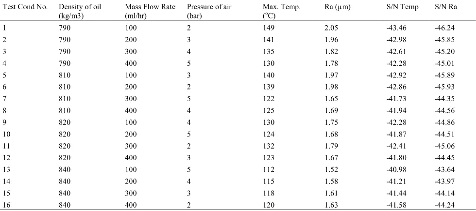
Holes have been drilled in the cutting inserts for a diameter of 2mm and to depth of 2mm at a distance of 5mm ahead of cutting edge in each cutting insert using Electric Discharge Machining. K–type thermocouples of specifications: Diameter: 2mm; Length of wire: 1000mm; Temperature range: 0 – 900oC are brazed in to
the holes already drilled on the cutting inserts of specifications: CNMG 12 04 08. Then physical contact of thermocouples with the drilled surfaces has been ensured. The cutting insert with thermocouple brazed in 2mm diameter drilled hole is shown in Figure 2.
The four types of oil selected to be atomized over the cutting zone of cutting insert during machining are NAC 22, Amul Cut 4C, NAS 22 and NACS 32. The technical data of selected oil are presented in Table 2. The container used to store the oil is calibrated using a standard burette of 50 ml capacity. The spray nozzle having the mixing chamber to mix air and oil has been fabricated. The container which is fully closed with a vent hole in order to avoid contamination is conveniently supported by a stand which is incorporated with dampers to avoid the transfer of vibration to the container.
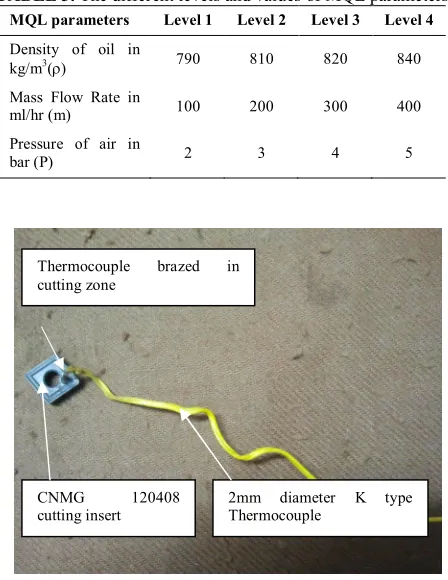
In machining there are various factors of MQL like thermal conductivity of cutting fluid, density of cutting fluid, viscosity of cutting fluid, mass flow rate of cutting fluid, pressure of air, etc., that affect the machining performance and cutting zone temperature. Among these parameters, density of cutting fluid, mass flow rate of air and pressure of air are the MQL parameters randomly selected for this study. Some of the preliminary experiments were conducted to identify the minimum value and maximum value of mass flow rate and pressure of air. When the mass flow rate of fluid and pressure of air were less than 100 ml/hr and 2 bar respectively, there is a rise in cutting zone temperature.
The reason may be due to inadequate adhesiveness of fluid with the cutting zone and thus the fluid evaporates before transferring the heat from cutting zone. Furthermore, when the mass flow rate of fluid and pressure of air were above 400 ml/hr and 5 bar respectively, it was found that cutting zone temperature increases. The reason is the cutting fluid could not have the enough time to have the contact with the cutting zone to remove the heat generated. Hence, mass flow rate of 100 ml/hr and pressure of 2 bar were identified as minimum values and mass flow rate of 400 ml/hr and pressure of 5 bar were identified as maximum value. The different levels and values of the selected MQL parameters are presented in Table 3.
TABLE 3. The different levels and values of MQL parameters
MQL parameters Level 1 Level 2 Level 3 Level 4
Density of oil in
kg/m3(r) 790 810 820 840
Mass Flow Rate in
ml/hr (m) 100 200 300 400 Pressure of air in
bar (P) 2 3 4 5
Figure 2. Thermocouple wire brazed in CNMG cutting insert
TABLE 2. Technical data of selected oil
S.No. Test Unit Test Method Specification of Cutting Oil
NAC 22 Amul Cut 4C NAS 22 NACS 32 1 Colour NA Visual Bright Amber
2 Clarity NA Visual Clear
3 Density at 32°C Kg/m3 ASTM D 1298 790 810 820 840
4 Kinematic Viscosity at 40°C Centi- Stokes ASTM D 445 29.2 30.1 31.6 33.2 5 Flash Point Degree C ASTM D 92 150 170 180 200
Thermocouple brazed in cutting zone
CNMG 120408
Figure 3. Experimental set up with the fabricated mixing chamber
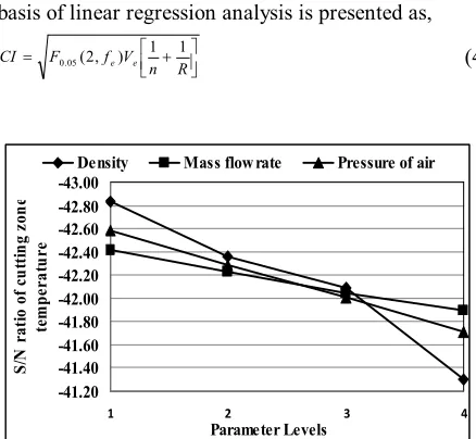
TABLE 4. Experimental test conditions and observed data
Test Cond No. Density of oil (kg/m3)
Mass Flow Rate (ml/hr)
Pressure of air (bar)
Max. Temp.
(oC) Ra (µm) S/N Temp S/N Ra
1 790 100 2 149 2.05 -43.46 -46.24
2 790 200 3 141 1.96 -42.98 -45.85
3 790 300 4 135 1.82 -42.61 -45.20
4 790 400 5 130 1.78 -42.28 -45.01
5 810 100 3 140 1.97 -42.92 -45.89
6 810 200 2 139 1.98 -42.86 -45.93
7 810 300 5 122 1.65 -41.73 -44.35
8 810 400 4 125 1.69 -41.94 -44.56
9 820 100 4 130 1.75 -42.28 -44.86
10 820 200 5 124 1.68 -41.87 -44.51
11 820 300 2 132 1.79 -42.41 -45.06
12 820 400 3 123 1.67 -41.80 -44.45
13 840 100 5 112 1.52 -40.98 -43.64
14 840 200 4 115 1.58 -41.21 -43.97
15 840 300 3 118 1.61 -41.44 -44.14
16 840 400 2 120 1.63 -41.58 -44.24
Each machining operation is carried out for the pre determined duration of 180 seconds in order to have the flank wear of less than 0.4 mm. The experimental setup during machining to record and to monitor the temperature change of cutting zone along with the fabricated mixing chamber is shown in Figure 3. The turning parameters such as cutting speed, feed rate and depth of cut are 150 m/min, 0.15 mm/rev and 0.1mm, respectively. The peak values of temperature during machining is recorded using digital temperature indicator of specifications, Make: SELEC DTC303;
Temperature range:0 – 900oC. The surface roughness of
the finished product has been measured using surface roughness tester of specifications: Model: Surtronic 3+; Traverse speed: 1 mm/sec; Display: LCD matrix 2 lines x 16 characters, alphanumeric; Parameters: Ra, Rq, Rz,
Ry and Sm; Calculation time: Less than reversal time.
The calculated numbers of experiments at different test conditions are performed with sixteen fresh cutting edges of same specifications. After completing the experiments, the arithmetic average surface roughness value of each machined surface is measured which is not permitting to exceed 3 microns. The experimental test conditions and observed data of cutting zone temperature and surface roughness (both Raw and S/N values) are presented in Table 4.
4. RESULTS AND DISCUSSION
The individual effect of density of cutting fluid on cutting zone temperature corresponding to 790 kg/m3 is
calculated as,
S/N ratio = [(-43.46-42.98-42.61-42.28) / 4] = -42.83
The individual effects of MQL parameters on cutting zone temperature is graphically represented in Figure 4. The S/N ratio values of the objective for all the test conditions are calculated and presented in Table 4. The best levels of selected MQL parameters (maximum S/N ratio values) are identified as,
Density of oil,(r4) = 840 kg/m3
Mass flow rate of oil, (m4) = 400 ml/hr
Pressure of air, (P4) = 5 bar
With the identified best levels of MQL parameters, a validation experiment is conducted for validation. In the validation experiment, maximum temperature is recorded as 109oC which is lower than that of the other
temperature values shown in Table 3. The corresponding S/N ratio value of the objective in validation experiment is calculated as,
S/N value of Temperature = -40.75
For verifying the validated result of cutting zone temperature through linear regression analysis, the estimated mean is calculated as,
m
em m P T
T =r+ + -2 (3)
where,
Tem = Estimated mean of temperature
r = Mean of temperature corresponding to density of oil
m = Mean of temperature corresponding to mass flow rate of oil
P = Mean of temperature corresponding to pressure of air
Tm = Overall mean of temperature.
From Table 3, the mean values of the parameters are substituted in (3) and Tem is calculated as,
Tem = (-41.30) + (-41.90) + (-41.71) – 2(-42.15)
= - 40.61
The regression table for cutting zone temperature is developed using linear regression analysis as shown in Table 5.
A Confidence Interval; CI for the prediction of mean temperature based on the validation experiment on the basis of linear regression analysis is presented as,
úû ù êë é + =
R n V f F
CI e e
1 1 ) , 2 (
05 .
0 (4)
Figure 4. Best values of MQL parameters for the minimum value of cutting zone temperature
TABLE 5. Summary output – Linear Regression – Temperature
ANOVA
df SS MS F Significance F
Regression 3 7.063055 2.354352 108.5475 5.82E-09 Residual 12 0.260275 0.02169
Total 15 7.32333
Coefficients Std Error t Stat P-value
Intercept -68.3952 1.670913 -40.9328 2.93E-14
x r 0.030444 0.002042 14.90655 4.17E-09
x m 0.001724 0.000329 5.235298 0.000209
x P 0.287145 0.032931 8.71947 1.54E-06
-43.00 -42.80 -42.60 -42.40 -42.20 -42.00 -41.80 -41.60 -41.40 -41.20
1 2 3 4
Parameter Levels
S/
N
r
at
io
o
f c
u
tt
in
g
zo
n
e
te
m
pe
ra
tu
re
where,
fe - Error degrees of freedom (12 from Table 5)
F0.05 (2, fe) - F ratio required for risk (2, 12)
= 3.89 from standard “F” table as in Harry Frank et al. [24]
Ve - Error variance (0.02169) from Table 5
R - Number of repetitions for confirmation test (1) N - Total number of experiments = 16
n - Effective number of replications
=N / (1 + degrees of freedom associated with temperature)
=16 / (1 + 15) =1
By substituting these values in (4), the value of CI for the temperature based on regression analysis is calculated as,
CI = {3.89 x 0.02169 x [(1/1) + (1/1)]} 1/2 = 0.41
The 95% confidence interval of the optimal temperature in validation test is verified as,
(Tem – CI) < Tcon < (Tem + CI)
-41.02< Tcon < -40.2
where, Tcon is the maximum temperature recorded in the
confirmation experiment.
The result of confirmation test shows that the S/N value of temperature is -40.75 which is in between (Tem
– CI) and (Tem + CI). The validated temperature is thus
confirmed by the above calculations.
The % contribution of an individual parameter on the S/N-cutting zone temperature is calculated by dividing the best value of the particular parameter (from Figure 2) by the sum of all the best values of other parameters multiplied by hundred. The individual % contribution of all parameters on the S/N-cutting zone temperature is shown below:
Density of fluid = 41.30 100 33.06 %
41.30 41.90 41.71x
- =
- -
-Mass flow rate= 33.54 % Pressure of air = 33.39 %
From the above calculations it is confirmed that, the density of cutting fluid is less significant on the S/N-cutting zone temperature followed by other parameters. The mass flow rate of cutting fluid is highly significant on the S/N-cutting zone temperature.
Empirical model for the cutting zone temperature based on linear regression model is developed as,
(5)
( 68.3952 (0.030444 ) (0.00172 )
(0.28714LR ))
T x xm
xP
r
= - + + +
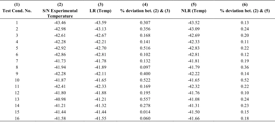
The percentage deviations between the predicted and experimental data of cutting zone temperature at different test conditions are presented in Table 6.
By substituting the corresponding values of parameters of test condition number 8 in (5), the predicted S/N value of temperature is obtained as -41.89. The comparison between S/N ratio of experimentally obtained temperature values and linear regression model values is shown in Figure 5.
Experimental S/N value of temperature corresponding to the test condition number 8 is -41.94. The percentage deviation between the S/N values of experimentally observed and predicted cutting zone temperature for the test condition number 8 is calculated as,
. .
% 100
.
EmpValue ExpValue
Deviation x
EmpValue
-=
41.89 ( 41.94) 100 0.097%
41.89 x
-
-= =
-TABLE 6. Regression model values – Cutting Zone Temperature
(1) Test Cond. No.
(2) S/N Experimental
Temperature
(3) LR (Temp)
(4)
% deviation bet. (2) & (3)
(5) NLR (Temp)
(6)
% deviation bet. (2) & (5)
1 -43.46 -43.59 0.307 -43.52 0.13
2 -42.98 -43.13 0.356 -43.09 0.24
3 -42.61 -42.67 0.168 -42.69 0.20
4 -42.28 -42.21 0.141 -42.33 0.11
5 -42.92 -42.70 0.516 -42.83 0.22
6 -42.86 -42.81 0.102 -42.81 0.12
7 -41.73 -41.78 0.132 -41.81 0.19
8 -41.94 -41.89 0.097 -41.79 0.36
9 -42.28 -42.11 0.400 -42.22 0.14
10 -41.87 -41.65 0.522 -41.65 0.52
11 -42.41 -42.33 0.169 -42.32 0.22
12 -41.80 -41.88 0.195 -41.76 0.10
13 -40.98 -41.21 0.557 -41.08 0.24
14 -41.21 -41.32 0.278 -41.31 0.23
15 -41.44 -41.44 0.014 -41.50 0.15
Figure 5. Comparison between S/N ratio values of cutting zone temperature and predicted values using linear regression analysis
Figure 6. Comparison between S/N ratio values of cutting zone temperature and predicted values using non linear regression analysis
Figure 7. Comparison between the % deviation of Linear Regression and Non Linear Regression from experimental S/N values of temperature
For verifying the validated result of cutting zone temperature based on non linear regression analysis, Tem
is calculated and found as -40.61. The non linear regression data for temperature is developed is presented in Table 7.
A Confidence Interval for the prediction of temperature based on the validation experiment on the
basis of Non Linear Regression model is calculated and found as, CI = 0.3794. The result of confirmation test shows that the S/N value of temperature is -40.75 which is in between -40.9894 and -40.2306. The validated temperature is thus confirmed by the above calculations. Empirical model for the cutting zone temperature based on non linear regression model is developed as,
6
( 51.58 (0.0093 ) (0.0094 ) (4.82947 )
(7.7 10 ) (0.0063 ) (0.00017 ))
LR
T x xm xP
x x xm x xP xmxP
r
r r
-= - + +
-- + - (6)
The comparison between S/N ratio of
experimentally obtained temperature values and non linear regression model values is shown in Figure 6. The Non Linear Regression model values of cutting zone temperature are already presented in Table 5.
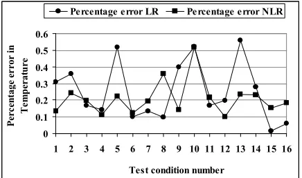
The comparison between % deviations of temperature in linear regression model with % error of temperature in non linear regression model for the prediction of cutting zone temperature using LR and NLR are shown in Figure 7.
Since the traditional optimization technique, Taguchi’s Design of Experiments identifies only the nearest levels of MQL parameters, it is decided to go for some of the non traditional optimization techniques such as Particle Swarm optimization, Simulated Annealing Algorithm and Differential Evolution techniques. They used to identify the exact values of MQL parameters for the minimization of cutting zone temperature by maintaining the value of surface roughness (constraint) well below 3.00 microns.
Even though the average percentage deviation of cutting zone temperature using non linear regression model is lesser than that of average percentage deviation of cutting zone temperature using linear regression model, the values of Objective Function from non traditional technique obtained using the non linear regression model were not satisfactory. Hence, the output obtained from non traditional technique using linear regression model only presented in this analysis.
As a first attempt, the Particle Swarm Optimization technique is used in this study to obtain the best global values of MQL parameters. The values of C1 and C2 in
Eq. 1 are tried and the optimal values for both are found to be 3. The different values of Objective Function (OF) by varying the number of populations are obtained as,
N = 5; OF = 0.68937 N = 10; OF = 0.68900 N = 15; OF = 0.69081 N = 20; OF = 0.69044 N = 25; OF = 0.69044 N = 30; OF = 0.69044 N = 35; OF = 0.69044 N = 40; OF = 0.69009 N = 45; OF = 0.69009 N = 50; OF = 0.69044
-44
-43
-42
-41
-40
1 2 3 4 5 6 7 8 9 10 11 12 13 14 15 16
Test condition number
S
/N R
at
io
o
f
T
em
p
er
at
u
re
Expeimental S/N - T Predicted S/N - T
-46 -45 -44 -43 -42 -41 -40
1 2 3 4 5 6 7 8 9 10 11 12 13 14 15 16
Test condition number
S
/N
Ra
tio
o
f
Te
m
p
er
atu
re
Experiental S/N - T Predicted NLR S/N - T
0 0.1 0.2 0.3 0.4 0.5 0.6
1 2 3 4 5 6 7 8 9 10 11 12 13 14 15 16
Test condition number
Per
ce
ntag
e
er
ro
r
in
T
em
p
er
at
u
re
From the above trials, with the population size of 10, the value of OF is 0.68900, which is lower than that of all values in other trials. The best values of selected parameters obtained using PSO, the S/N values of cutting zone temperature and surface roughness are presented in Figure 8.
As a next attempt, the best values of MQL parameters for the minimization of temperature are obtained using SAA. In SAA, the initial temperature (T) and decrement factor (d) are the two important parameters which govern the successful working of the simulated annealing procedure. If a larger initial value of ‘T’ (or) ‘d’ is chosen, it takes more number of iterations for convergence. On the other hand, if a small value of initial temperature ‘T’ is chosen, the search is not adequate to thoroughly investigate the search space before converging to the true optimum. Unfortunately, there are no unique values of the initial temperature (T), decrement factor (d) and number of iterations (n) that work for every problem.
However, an estimate of the initial temperature can be obtained by calculating the average of the function values at a number of random points in the search space.
Figure 8. Best levels of MQL parameters obtained, S/N values of cutting zone temperature and surface roughness obtained from PSO
A suitable value of ‘n’ can be chosen (usually between 2 and 200) depending on the available computing resource and the solution time. Decrement factor is left to the choice of the user. However, the initial temperature and subsequent cooling schedule require some trial and error efforts. Hence, different combinations of these two parameters have been analyzed and the Objective Function; OF are obtained for the following combinations. There are better results for different possible combinations of these two parameters; but, almost all the possible combinations have been tried out as,
Number of iterations, n = 200
T = 400o C, df = 0.1 and OF = 0.68895
T = 400o C, df = 0.2 and OF = 0.68894
T = 400o C, df = 0.3 and OF = 0.68892
T = 400o C, df = 0.4 and OF = 0.68896
T = 400o C, df = 0.5 and OF = 0.68895
T = 400o C, df = 0.6 and OF = 0.68896
T = 400o C, df = 0.7 and OF = 0.68893
T = 400o C, df = 0.8 and OF = 0.68894
T = 400o C, df = 0.9 and OF = 0.68891
T =1000o C, df = 0.9 and OF = 0.68894
When the temperature and decrement factor are maintained at 400oC and 0.9, the minimum value of OF
(0.68891) is obtained. The temperature of 1000o C does
not improve the value of OF, and hence this temperature is not considered in this analysis. The best values of selected parameters obtained using SAA and the S/N values of cutting zone temperature and surface roughness are presented in Figure 9.
As a last attempt, the best values of parameters for the minimization of cutting zone temperature are obtained using Differential Evolution technique. For the population size of 35, scaling factor of 0.4 and crossover constant of 0.7, the S/N value of temperature is -40.696915 which is greater than that of all other values in other trials.
TABLE 7. Summary output – Non Linear Regression – Temperature
ANOVA
df SS MS F Significance F
Regression 6 7.170 1.195 70.402 4.72E-07
Residual 9 0.152 0.0169
Total 15 7.32
Coeff Std Error t Stat P-value
Intercept -51.5184 9.085 -5.670 0.0003
x r 0.009325 0.011 0.818 0.434
x m 0.009498 0.020 0.453 0.661
x P -4.82947 2.093 -2.306 0.046
x rxm -7.7E-06 2.57E-05 -0.300 0.770
x rxP 0.006318 0.0025 2.463 0.035
Figure 9. Best values of MQL parameters obtained, S/N values of cutting zone temperature and surface roughness obtained from SAA
Figure 10. The comparison between predicted S/N cutting zone temperature values obtained using PSO, SAA and DE
Here, the convergence starts at iteration number 79. For the population size of 15 and 40, same S/N value of temperature is obtained. However, the convergence starts at 109 and 86 respectively. Hence, the result obtained using the combinations with NP of 15, F of 0.4, CR of 0.7 and NP of 40, F of 0.4 and CR = 0.7 are not presented in this study.
The various trials of experiments has been conducted by varying the size of populations (NP) from 10 to 50 with the interval of 5, scaling factor (F) from 0.4 to 0.9 with the interval of 0.1 and Crossover constant (CR) from 0.1 to 0.9 with the interval of 0.1. The S/N value of temperature by varying the number of populations, scaling factor and crossover constant using empirical model is shown as,
NP = 10; F = 0.4; CR = 0.6 Temp = -40.739 NP = 10; F = 0.4; CR = 0.7 Temp = -40.74 NP = 10; F = 0.4; CR = 0.8 Temp = -40.6974 NP = 15; F =0.4; CR = 0.7 Temp = -40.6969 NP = 35; F = 0.4; CR = 0.7 Temp = -40.6969 NP = 40; F = 0.4; CR = 0.7 Temp = -40.6969
When the number of population is greater than 10 the S/N value of cutting zone temperature is maximum (-40.6969) for all the combination of trials.
The comparison between predicted S/N values of cutting zone temperature obtained using PSO, SAA and DE are presented in Figure 10.
5. CONCLUSION
In this analysis, the values of cutting zone temperature during machining have been measured on-line and recorded for the selected MQL parameters at different test conditions. The following are the conclusions drawn:
1. The minimum value of cutting zone temperature obtained in the validation experiment from DoE is 109oC which is lower than that of all the experimental values by that of 2.67%.
2. Since in Figure 4, the trend between experimental S/N ratio values of cutting zone temperature is uniform with the predicted values of cutting zone temperature, it is well known that this developed model is possible to be used for the prediction of cutting zone temperature for all test conditions. 3. As the trend between experimental S/N ratio values
of cutting zone temperature is almost same with the predicted values of cutting zone temperature using non linear regression model in Figure 5, the predicted model using non linear regression model is also possible to be used for the prediction of cutting zone temperature for all test conditions.
4. From Figure 6, it is well defined that the non linear regression model shows a comparatively minimum deviation of cutting zone temperature when compared to linear regression model based on all test conditions.
5. The percentage improvement in S/N value of cutting zone temperature using PSO is 3.15% when compared with the maximum experimental S/N value of cutting zone temperature.
6. The percentage improvement in S/N value of cutting zone temperature using SAA is 3.209% when compared with the maximum experimental S/N value of cutting zone temperature.
7. The percentage improvement in S/N value of cutting zone temperature using DE is 3.255% when compared with the maximum experimental S/N value of cutting zone temperature.
8. The Differential Evolution technique is well suited to optimize the best combination of MQL parameters which gives the maximum S/N value of cutting zone temperature compared to other -42.6
-42.1
-41.6
-41.1
1 21 41 61 81 101 121 141 161 181
Iteration Number
S
/N
R
at
io
-
T
e
mp
er
at
u
re
traditional and non traditional optimization techniques.
6. REFERENCES
1. Paul, S., Dhar, N.R. and Chattopadhyay, A.B., “Beneficial effects of cryogenic cooling over dry and wet machining on tool wear and surface finish in turning AISI 1060 steel”, Journal of Material Processing Technology, Vol.116, No. 1, (2001), 44-48.
2. Sokovic, M. and Mijanovic, K., “Ecological aspects of the cutting fluids and its influence on quantifiable parameters of the cutting processes”, Journal of Material Processing Technology,
Vol. 109, No. 1-2, (2001), 181-189.
3. Diniz, A.E., Ferreira, J.R. and Filho, F.T., “Influence of refrigeration/lubrication condition on SAE 52100 hardened steel turning at several cutting speeds”, International Journal of Machine Tools & Manufacture, Vol. 43, No. 3,(2003), 317-326.
4. Machado, A.R. and Wallbank, J., “The effect of extremely low lubricant volumes in machining”, Wear, Vol. 210, No. 1-2, (1997), 76-82.
5. Rahman, M., Senthil Kumar, A. and Manzoor-Ul-Salem, “Evaluation of minimal quantities of lubricant in end milling”,
International Journal of Advanced Manufacturing Technology, Vol. 18, No. 4, (2001), 235-241.
6. Braga, D.U., Diniz, A.E., Miranda, G.W.A. and Coppini, N.L., “Using a minimum quantity of lubricant (MQL) and a diamond coated tool in the drilling of aluminium-silicon alloys”, Journal of Materials Processing Technology, Vol. 122, No. 1, (2002), 127-138.
7. Tasdelen, B., Thordenberg, H. and Olofsson, D., “An experimental investigation on contact length during minimum quantity lubrication (MQL) machining”, Journal of Materials Processing Technology, Vol. 203, (2008), 221-231.
8. Rahman, K.M., “Effect of minimum quantity lubrication (MQL) in drilling commercially used steels”, M Eng Dissertation,
BUET, Bangladesh, (2004).
9. Kamata, Y. and Obikawa, T., “High speed MQL finish-turning of Inconel 718 with different coated tools”, Journal of Materials Processing Technology, Vol. 192, No. 193,(2007), 281-286.
10. Davim, J.P., Sreejith, P.S. and Silva, J., “Turning of brasses using minimum quantity of lubricant (MQL) and flooded-lubricant conditions”, Material Manufacturing Process, Vol. 22,(2007), 45–50.
11. Kuan-Min, L. and Steven, Y. L., “Performance profiling of minimum quantity lubrication in machining”, International Journal of Advanced Manufacturing Technology, Vol. 35, (2007), 226-233.
12. Khan, M.M.A., Mithu, M.A.H. and Dhar, N.R., “Effects of minimum quantity lubrication on turning AISI 9310 alloy steel using vegetable oil-based cutting fluid”, Journal of Materials Processing Technology, Vol.209, (2009), 5573-5583.
13. Gaitonde, V.N., Karnik, S.R. and Davim, P., “Selection of optimal MQL and cutting conditions for enhancing machinability in turning of brass”, Journal of Materials Processing Technology, Vol. 204, (2008), 459-464.
14. Dhar, N.R., Ahmed, M.T. and Islam, S., “An experimental investigation on effect of minimum quantity lubrication in machining AISI 1040 steel”, International Journal of Machine Tools & Manufacture, Vol. 47, (2007), 748-753.
15. Dhar, N.R., Islam, M.W., Islam, S. and Mithu, M.A.H., “The influence of minimum quantity lubrication (MQL) on cutting temperature, chip and dimensional accuracy in turning AISI 1040 steel”, Journal of Materials Processing Technology, Vol. 171, (2006), 93-99.
16. Yanming, L. and Chaojun, W., “Neural Network based Adaptive Control and Optimization in the Milling Process”,
International Journal of Advanced Manufacturing Technology, Vol. 15, No. 11, (1999), 791-795.
17. Vijayakumar, K., Prabhaharan, G., Asokan, P. and Saravanan, R., “Optimization of multi-pass turning operations using ant colony system”, International Journal of Machine Tools and Manufacture, Vol. 43, (2003), 1633-1639.
18. Milfelner, M., Zuperl, U. and Cus, F., “Optimization of cutting parameters in high speed milling process by GA”, International Journal of Simulation and modeling, Vol. 3, No. 4, (2004), 121-131.
19. Asokan, P., Baskar, N., Babu, K., Prabhaharan, G. and Saravanan, R., “Optimization of surface grinding operations using Particle Swarm Optimization Technique”, ASME Journal of Manufacturing Science and Engineering,Vol. 127, (2005), 885-892.
20. Jerald, J., Asokan, P., Prabhaharan, G. and Saravanan, R., “Scheduling Optimization of Flexible Manufacturing Systems using Particle Swarm Optimization algorithm”, International Journal of Advanced Manufacturing Technology, Vol. 25, (2005), 964-971.
21. Goldberg, D.E., “Genetic Algorithms in Search. Optimization and Machine Learning”, Addison-Wesley Longman Publishing Co., Boston, MA, USA (1989).
22. Price, K. and Storn, R., “Differential Evolution – A simple evolution strategy for fast optimization”, Dr. Dobb’s Journal,
Vol. 22, No. 4, (1997), 18 – 24.
23. Tamizharasan, T., Kingston Barnabas, J. and Pakkirisamy, V., “Optimisation of cooling fin parameters in turning by using DoE, AGA and SAA based on cutting zone temperature”,
International Journal of Machining and Machinability of Materials, Vol. 11, No. 2, (2012), 115-136.
Optimization of Minimum Quantity Liquid Parameters in Turning for the
Minimization of Cutting Zone Temperature
T. Tamizharasana, J. Kingston Barnabasb
aPrincipal, TRP Engineering College, Irungalur, Tiruchirappall - 621 105
bDepartment of Mechanical Engineering, Anjalai Ammal Mahalingam Engineering College, Kovilvenni, Tiruvarur District – 614 403
P A P E R I N F O
Paper history: Received 19 July 2011
Received in revised form 16 April 2012 Accepted 17 September 2012
Keywords:
Cutting Zone Temperature Surface Roughness
Taguchi’s Design Of Experiments Particle Swarm Optimization Simulated Annealing Algorithm Differential Evolution هﺪﯿﮑﭼ رد لﺎﺣ ﺮﺿﺎﺣ هدﺎﻔﺘﺳا زا شﺮﺑ ﻊﯾﺎﻣ رد ﻊﯾﺎﻨﺻ ،يﺪﯿﻟﻮﺗ ﺎﺑ ﻪﺟﻮﺗ ﻪﺑ يﺎﻫ ﯽﮔدﻮﻟآ ﻂﯿﺤﻣ ﯽﺘﺴﯾز و ﻞﺋﺎﺴﻣ ﻂﺒﺗﺮﻣ ﺎﺑ ﺖﻣﻼﺳ نﺎﻨﮐرﺎﮐ اﺰﻠﮑﺸﻣ ﺪﺷﺎﺑ ﯽﻣ . ﻦﯿﻨﭽﻤﻫ ﻪﺑ ﻞﻗاﺪﺣ زا هدﺎﻔﺘﺳا نﺪﻧﺎﺳر شﺮﺑ ،ﻊﯾﺎﻣ ﺮﺠﻨﻣ ﻪﺑ ﻪﻓﺮﺻ ﯽﯾﻮﺟ رد زا هدﺎﻔﺘﺳا يﺎﻫ ﻪﻨﯾﺰﻫ
ناور ﺎﻫ هﺪﻨﻨﮐ و ﺰﯿﻤﺗ نﺎﻣز ﺶﻫﺎﮐ ندﺮﮐ ﻦﯿﺷﺎﻣ ،تﻻآ راﺰﺑا و تﺎﻌﻄﻗ يرﺎﮐ ﺪﺷﺎﺑ ﯽﻣ . مﻮﻬﻔﻣ راﺪﻘﻣ ﻞﻗاﺪﺣ يرﺎﮑﻧاور (MQL) زا ﮏﯾ ﻪﻫد ﻞﺒﻗ ﻪﺑ رﻮﻈﻨﻣ ﻪﺒﻠﻏ ﺮﺑ ﺐﯾﺎﻌﻣ ﮏﻨﺧ لﺎﯿﺳ هﺪﻨﻨﮐ ﻪﺑ ﺖﺳا ﻪﺘﻓر رﺎﮐ .
ﻦﯾا ﻖﯿﻘﺤﺗ ﯽﺳرﺮﺑ ﻪﺑ يﺎﻫﺮﺘﻣارﺎﭘ MQL ياﺮﺑ ﻪﺑ ﻞﻗاﺪﺣ نﺪﻧﺎﺳر ﻪﺟرد تراﺮﺣ ﻪﻘﻄﻨﻣ ،شﺮﺑ ﺎﺑ ﻪﺟﻮﺗ ﻪﺑ يﺮﺑز ﺢﻄﺳ ﻪﺑ ناﻮﻨﻋ ﯽﻣ ،هﺪﻨﻨﮐ دوﺪﺤﻣ ﻞﻣﺎﻋ ﮏﯾ
دزادﺮﭘ . . ﺮﺘﻣارﺎﭘ يﺎﻫ بﺎﺨﺘﻧا هﺪﺷ يﺎﻫ MQL رد رﺎﻬﭼ ﺢﻄﺳ توﺎﻔﺘﻣ ﺖﺳا . ﺮﺜﮐاﺪﺣ راﺪﻘﻣ ﻪﺟرد تراﺮﺣ رد نﺎﻣز ﯽﻃ
يرﺎﮑﻨﯿﺷﺎﻣ رد ﺎﻫ ﺖﺴﺗ ﯽﻣﺎﻤﺗ ، رد L16 ﻢﺋﺎﻗ ﻪﯾواز ﺖﺒﺛ ﺖﺳا هﺪﺷ . راﺪﻘﻣ ﻦﯾﺮﺘﻬﺑ زا يﺎﻫﺮﺘﻣارﺎﭘ بﺎﺨﺘﻧا هﺪﺷ MQL ياﺮﺑ ﻪﺑ ﻞﻗاﺪﺣ نﺪﻧﺎﺳر ﻪﺟرد تراﺮﺣ ﻪﻘﻄﻨﻣ ،شﺮﺑ ﺎﺑ هدﺎﻔﺘﺳا زا ﯽﺣاﺮﻃ ﯽﭼﻮﮔﺎﺗ زا ،هﺪﺷ مﺎﺠﻧا يﺎﻫ ﺶﯾﺎﻣزآ ﺺﺨﺸﻣ ﺪﺷ . ﺶﯾﺎﻣزآ رﺎﺒﺘﻋا ﯽﺠﻨﺳ ﺎﺑ ﺢﻄﺳ ،ﺺﺨﺸﻣ زا يﺎﻫﺮﺘﻣارﺎﭘ مﺎﺠﻧا هﺪﺷ ﻪﻘﻄﻨﻣ يﺎﻣد ﻪﺑ ﻪﺟﻮﺗ ﺎﺑو شﺮﺑ ﺖﺒﺛ هﺪﺷ ﺖﺳا . ﻦﯾا ﻪﯾﺰﺠﺗ و ﻞﯿﻠﺤﺗ ﺮﺘﺸﯿﺑ ﻪﺑ طﻮﺑﺮﻣ ياﺮﺟا ﻪﻨﯿﻬﺑ يزﺎﺳ مﺎﺣدزا تارذ ) PSO ( ، ﻢﺘﯾرﻮﮕﻟا ﻪﯿﺒﺷ يزﺎﺳ ﮓﻨﯿﻠﯿﻧآ ) SAA ( و ﻞﻣﺎﮑﺗ ﻞﯿﺴﻧاﺮﻔﯾد ) DE ( ياﺮﺑ ﻪﺑ ﻞﻗاﺪﺣ نﺪﻧﺎﺳر ﻪﻘﻄﻨﻣ يﺎﻣد ﺖﺳا هﺪﺷ مﺎﺠﻧا شﺮﺑ